Disclaimer: These notes have not been subjected to the usual scrutiny reserved for formal publications.
6.1
Review of the last lecture
General setup• For each roundt, every expert igives a predictionxt
i∈ {0,1};
• An algorithm predicts ˆyt∈ {0,1}, based on experts’ predictions;
• Natural reveals yt∈ {0,1}.
Halving algorithm In last lecture, we proved the following claim:
Claim 6.1 There exists an algorithm which makes fewer thanlog2N mistakes by an arbitrary timeT >0,
MT(Alg) = T X t=1 1[ ˆyt6=yt]≤log 2N
This claimed is proved by considering thehalving algorithm. Recall that the proof was sketched as follows.
Proof: LetCt+1 be the index set of experts who have not yet made mistakes in the first t rounds. We have, C1={1,2,3, ..., N} Ct+1=Ct\ {i:xti 6=y t } ˆ yt= round 1 |Ct| X i∈Ct xti !
We can observe that once the algorithm made a mistake, the majority (no less than half) of experts must made a wrong prediction. Then the number of the remaining experts in the next round would be reduced by at least half. ˆ yt6=yt =⇒ |Ct+1|/|Ct| ≤1 2 =⇒ |Ct+1| ≤ |C1|( 1 2) Mt
Suppose the algorithm finds the perfect expert after round T, this means|CT+1| ≤1. Then the maximum
MT satisfiesMT ≤log2N, whereN is the number of experts in the first round.
6.2
The case with multiple choices
Let’s now consider a motivating example of betting the winning team of a tournament. Assume that there arenteams. On each round, two teamsitandjtplay a match. An algorithm aims predicting the outcome
of the match: whetheritbeatsjtor vice versa. Assume that each game has only one winner, eitheritorjt. Assume that there exists a permutation of all teamsπ∗∈ Sn, which specifies the outcome of all matches.
(HereSn represents the set of all permutations on [n].) Specifically,it beatsjtif and only if π(it)≥π(jt).
Intuitively, there is an absolute ranking of the teams that specifies the outcome of the result. Now, we need an algorithm that minimizes the total number of mistakes.
Claim 6.2 There exists an algorithm that satisfies the following bound: Ct≤log2{n!}.≤nlog2n
whereCtis the smallest number of mistakes that an algorithm makes before time t.
The idea is to consider a committee ofn! experts. Each of them corresponds to a permutation π∈ Sn,
and predict the outcome of the game betweenitandjt according to whetherπ(it)> π(jt), i.e., xtπ=1[π(it)> π(jt)].
Also, the decision by Nature can be described by permutationπ∗,
yt=1[π∗(it)> π∗(jt)].
Now, we transform the setup of this problem to that of the Halving Algorithm, and that Claim 6.2 follows immediately from Claim 6.1.
Remarks
• The students are encouraged to think about if/how the above algorithm can be performed efficiently. • By Sterling formula, the expression log{n!} is actually in the order of nlogn. Notice that the order
is the same with that of the comparisons you need in sort a sequence of size n. However, a major difference is that in sorting problem, we can arbitrarily select the two elements to compare. In our “experts” setup, however, every pair of teams is selected based on the game played, and the measure is the number of mistakes instead of the number of comparisons.
• We might need a smoother algorithm than Halving Algorithm that it might not expire experts once they made a mistake and is similar to a weighted majority vote, as will be introduced in the next section.
6.3
Weighted Majority Algorithm
Now let’s consider the case where no expert is “perfect”, that is, all experts are subject to making mistakes. Let MT(i) := PT
t=11[x
t i 6=y
t] be the number of incorrect guesses from expert i up to time T and MT(Alg) := P
T t=11[ˆy
t6=yt] be the total number of incorrect guesses generated from the algorithm that
based on the answers of the experts.
We will describe “weighted majority algorithm” (WMA) below, which can be regarded a “softer” or “smoother” version of the Halving algorithm. In WMA, making mistakes will not get an expert “fired”. Instead, a mistake downgrade the weight of this expert’s guesses. In this sense, the Halving Algorithm is a special case of it, as each expert are assigned with zero or one weight, and making each mistake drops its weight down to zero. It was formally proposed in 1994. However, similar idea appeared around 1950s/1960s.
Weighted Majority Algorithm Let there beN experts in total, and theith expert make predictionxt i
at timet. WMA sets weightwt
i for expertiat each timet, and predicts the output using Algorithm 1 based
on the experts’ prediction.
The following Theorem 6.3 gives an upper bound onMT(WMA), the number of wrong decisions ˆytgiven
by the WMA from time 1 toT.
Theorem 6.3 For any sequence of data~x1, . . . , ~xt andy1, . . . , yt, we have MT(WMA)≤ 2
εlog (N) + 2(1 +ε)MT(i)
Algorithm 1Weighted Majority Algorithm Initializew1
i ←1,∀i= 1, . . . , N; fort= 2, . . . , T do
Generate prediction at timet by the weighted average of all experts
ˆ yt←round PN i=1w t ixti PN i=1w t i ! ,
Update the weight of all experts with
wti+1←wit(1−ε)1xti6=yt. end for
Several remarks on the WMA algorithm and Theorem 6.3:
• As the statement in the above theorem holds for every expert, it naturally holds for the “best” expert among allN experts.
• As we select ε= 1, the WMA algorithm reduces to Halving Algorithm and thus also gives an error bound for it. This bound is very similar to the one presented in Lecture 5, only up to a constant factor. In fact, under the setting that there exists an expertiwho always makes correct guess, we have
MT(i) = 0, and thus MT(WMA)≤2 loge(N).
• Consider that you have N machine learning methods to predict the outcome, and you do not know which method performs the best. The theorem here implies that as the number of observationsT → ∞, you can always construct an algorithm so that MT(Alg) increases at the same order as MT(i), where
i represents the algorithm with the best performance. (Note that 2 loge(N/ε) is neligible as T → ∞). Moreover, this algorithm is constructed according to the WMA.
• The WMA is similar to ensemble learning methods such asboosting, though the latter is more complex. The remaining part of this lecture proves Theorem 6.3. We first need the following lemma:
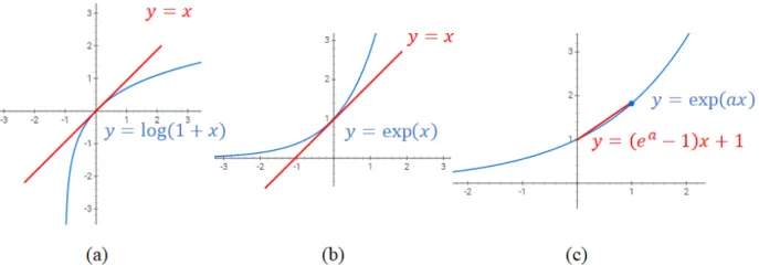
Lemma 6.4 The inequalities below hold: 1. log(1 +x)≤xfor all x∈R; 2. 1 +x≤exp(x)for allx∈R;
3. exp(ax)≤1 + (ea−1)xfor all x∈[0,1];
4. (Challenge Problem) : −log(1 +x)≤ −x+x2 for allx∈[−1/2,0].
Proof:
• The inequality 1 and 2 can be derived from the concavity and convexity of y = log(1 +x) and
y = exp{x}, respectively. The tangent line of y = log(1 +x) at point x = 0 is y = x, and thus log(1 +x)≤x. The tangent line ofy= exp{x}at pointx= 0 isy=x+ 1, and thus exp{x} ≥x+ 1. These two inequalities are illustrated in the first two plots in Figure 6.1.
• The inequality 3 results from the convexity of function y = exp{ax}. As shown in the last plot in Figure 6.1, we have
(1−x) exp(a·0) +xexp(a·1)≥exp{a·[0·(1−x) + 1·x]},
which indicates
Figure 6.1: Illustrations of the proof of Lemma 6.4
• The inequality 4 is left as an exercise.
The Lemma 6.4 will be used to prove Theorem 6.3. The proof also relies on the properties of the potential function, as described below.
Definition 6.5 (Potential function) The functionΦt:=P N i=1w
t
i is called thepotential function. Proposition 6.6 Based on the WMA algorithm, we have the following facts on the potential function:
1. (Initial condition)Φ1=N;
2. (Lower bound)ΦT+1≥wiT+1= (1−ε)MT(i); 3. (Upper bound)ΦT+1≤N(1−ε/2)
MT(WMA).
Proof:
1. The result follows immediately from the initial condition wi1= 1,∀i. 2. Trivial
3. To prove the upper bound, we need to show
Claim 6.7 If the WMA errs at timet, then
Φt+1≤(1−ε/2)Φt.
Proof: In class, Prof. Abernethy gave an illustrative interpretation1. Based on its idea, a formal proof is provided here. Let It ={i : xti 6= yt}. We first show that P
i∈Itw t i ≥ 1 2 PN i=1w t i. When y t = 0, 1ConsiderN objects in the space whose volumes arewt
i, i= 1, . . . , N at timet. They are colored as black and white, and
the black objects takes over half of the entire volume. At timet+ 1, the black objects shrink by factor 1−ε. Then the total size of the objects shrink by a factor at least (1−ε/2).
that WMA errs indicates that ˆyt = 1, i.e., It ={i: xt i = 1} and P i∈Itwti PN i=1wti >1/2; when yt = 1, that
WMA errs indicates that ˆyt = 0, i.e., It ={i : xt
i = 0} and P i∈Ictw t i PN i=1wit
< 1/2, which further implies
P i∈Itw t i≥ PN i=1wit. Now Φt+1= N X i=1 wti+1 =X i∈It wti+1+X i∈Ic t wti+1 =X i∈It (1−ε)wit+X i∈Ic t wit =X i∈It (1−ε)wit+ N X i=1 wti−X i∈It wti ! =(−ε)X i∈It wti+ N X i=1 wit ≥ −ε 2 N X i=1 wti+ N X i=1 wti=1−ε 2 Φt
With the Claim 6.7, we know ΦT+1≤(1−ε/2)1[y T6=ˆyT] ΦT ≤ · · · ≤ T Y t=1 (1−ε/2)1[yt6=ˆyt]Φ1=N(1−ε/2) PT t=11[ˆy t6=yt] =N(1−ε/2)MT(WMA)
Note that we used Item 1 in Proposition 6.6, Φ1=N.
Finally, we prove the Theorem 6.3 below by integrating 2 and 3 of Proposition 6.6, as well as Lemma 6.4.
Proof: The upper bound and lower bound of Proposition 6.6 gives (1−ε)MT(i)≤Φ
T+1≤N(1−ε/2)MT(WMA) Take negative-log on both sides, we have
−MT(i) log(1−ε)≥ΦT+1≥ −MT(WMA) log (1−ε/2)−logN By Inequality 4 in Lemma 6.4,
MT(i)(ε+ε2)≥ −MT(i) log(1−ε); By Inequality 1 in Lemma 6.4,
−MT(WMA) log (1−ε/2)−logN ≥ −logN+ (ε/2)MT(WMA).
Combine the above three inequalities, we have
Divide each side of the above inequality byε/2, we have
MT(W M A)≤2