(will be inserted by the editor)
On-the-Fly Model Checking for Extended Action-Based
Probabilistic Operators
Radu Mateescu and Jos´e Ignacio Requeno
Univ. Grenoble Alpes, Inria, CNRS, LIG, F-38000 Grenoble, France and University of Zaragoza, 50009 Zaragoza, Spain Received: date / Revised version: date
Abstract. The quantitative analysis of concurrent sys-tems requires expressive and user-friendly property lan-guages combining temporal, data handling, and quanti-tative aspects. In this paper, we aim at facilitating the quantitative analysis of systems modeled as PTSs ( Prob-abilistic Transition Systems) labeled by actions contain-ing data values and probabilities. We propose a new reg-ular probabilistic operator that specifies the probability measure of a path described by a generalized regular for-mula involving arbitrary computations on data values. This operator, which subsumes the Until operators of PCTL and their action-based counterparts, can provide useful quantitative information about paths having cer-tain (e.g., peak) cost values. We integrated the regular probabilistic operator into MCL (Model Checking Lan-guage) and we devised an associated on-the-fly model checking method, based on a combined local resolution of linear and Boolean equation systems. We implemented the method in the EVALUATOR model checker of the CADP toolbox and experimented it on realistic PTSs modeling concurrent systems.
1 Introduction
Concurrent systems, which are becoming ubiquitous nowadays, are complex software artifacts involving qual-itative aspects (e.g., concurrent behaviour, synchroniza-tion, data communication) as well as quantitative as-pects (e.g., costs, probabilities, timing information). The rigorous design of such systems based on formal methods and model checking techniques requires versatile tem-poral logics able to specify properties about qualitative and quantitative aspects in a uniform, user-friendly way. During the past two decades, a wealth of temporal logics dealing with one or several of these aspects were defined
and equipped with analysis tools [14, 7]. One of the first logics capturing behavioral, discrete time, and proba-bilistic information is PCTL (Probabilistic Computation Tree Logic) [29].
In this paper, we propose a framework for specify-ing and checkspecify-ing temporal logic properties combinspecify-ing actions, data, probabilities, and discrete time on PTSs (Probabilistic Transition Systems) [39], which are suit-able action-based models for representing value-passing concurrent systems with interleaving semantics. We con-sider here the class ofgenerative(also calledfully proba-bilitistic) PTSs [28], in which transition probability dis-tributions implicitly assign probabilities to the occur-rences of actions. These PTSs can be viewed as DTMCs (Discrete-Time Markov Chains) in which transitions are labeled by actions carrying probabilities, channel names, and data values sent between concurrent processes dur-ing handshake communication. We are interested mainly in action-based properties, in contrast with standard DTMCs [7, Chap. 10], where atomic propositions are attached to states. Our contributions are twofold.
Regarding the specification of properties, we pro-pose a new regular probabilistic operator, which spec-ifies the probability measure of a path (specified as a regular formula on actions) in a PTS. Several proba-bilistic logics have been proposed in the action-based setting. PML (Probabilistic Modal Logic) [39] is a vari-ant of HML (Hennessy-Milner Logic) [30] with modal-ities indexed by probabilmodal-ities, and was introduced as a modal characterization of probabilistic bisimulation on (generative) PTSs. GPL (Generalized Probabilistic Logic) [15] is a probabilistic variant of the alternation-free modal µ-calculus, able to reason about execution trees, and equipped with a model checking algorithm re-lying on the resolution of non-linear equation systems. Compared to these logics, our probabilistic operator is a natural (action-based) extension of the Until operator of PCTL: besides paths of the form a∗.b (the
action-based counterpart of Until operators), we consider more general paths, specified by regular formulas similar to those of PDL (Propositional Dynamic Logic) [24]. To handle the data values present on PTS actions, we rely on the regular formulas with counters of MCL (Model Checking Language) [48], an extension of first-order µ-calculus with programming language constructs. More-over, we enhance the MCL regular formulas with a gen-eralized iteration operator parameterized by data values, thus making possible the specification of complex (Tur-ing computable) paths in a PTS.
Regarding the evaluation of regular probabilistic for-mulas on PTSs, we devise an on-the-fly model check-ing method based on translatcheck-ing the problem into the simultaneous local resolution of a linear equation sys-tem (LES) and a Boolean equation syssys-tem (BES). For probabilistic operators containing dataless MCL regu-lar formulas, the sizes of the LES and BES are linear in the size of the PTS and linear (resp. exponential) in the size of the regular formula, depending whether it is deterministic or not. In the action-based setting, the de-terminism of formulas is essential for a sound translation of the verification problem to a LES. For general data handling MCL regular formulas, the termination of the model checking procedure is guaranteed for a large class of formulas (e.g., counting, bounded iteration, aggrega-tion of values, computaaggrega-tion of costs over paths, etc.) and the sizes of the equation systems depend on the data pa-rameters occurring in formulas. It is worth noticing that on-the-fly verification algorithms for PCTL were pro-posed only recently [40], all previous implementations, e.g., in PRISM [36] having focused on global algorithms. Our method provides on-the-fly verification for PCTL and its action-based variant PACTL, and also for PPDL (Probabilistic PDL) [35], which are subsumed by the regular probabilistic operator of MCL. We implemented the method in the EVALUATOR [48] on-the-fly model checker of the CADP toolbox [27] and experimented it on various examples of value-passing concurrent systems. Related work. Most of the works on action-based log-ics for quantitative analysis have concentrated on continuous-time models. CSL (Continuous Stochastic Logic) [4, 6] is a continuous-time variant of PCTL inter-preted on CTMCs (Continuous-Time Markov Chains). aCSL (action-based CSL) [31], interpreted on action-labeled CTMCs, is the action-based counterpart of CSL suitable for action-oriented modeling formalisms, such as stochastic process algebras. aCSL was defined in a way similar to ACTL (Action-based CTL) [49], which is the action-based counterpart of CTL [13]. In our set-ting, we can encode probabilistic versions of the ACTL operators, which are discrete-time counterparts of the time-bounded probability operators of aCSL. This logic was subsequently extended with regular operators simi-lar to those of PDL, leading to the strictly more expres-sive logic asCSL [5] interpreted on state- and
action-labeled CTMCs. The purpose of asCSL was to enable the specification of complex properties of finite compu-tations with real-time constraints. We had a similar mo-tivation for our regular probabilistic operator on PTSs, and we extended its expressiveness further by adding data-handling mechanisms.
In the state-based setting, the logic closest to ours is QuaTEx (Quantitative Temporal Expressions) [1], which combines constructs from PCTL and the rule-based query language EAGLE [8]. In QuaTEx, paths are de-scribed using recursive temporal operators with data pa-rameters, built over a next-time operator and conditional path expressions. QuaTEx queries are evaluated using statistical model checking on GSMPs (Generalized Semi-Markov Processes) produced from actor-based proba-bilistic programs written in the PMaude language [1]. Instead of recursive path formulas, our data-handling probabilistic operator extends the regular expressions over paths with a generalized iteration operator, yielding more concise specifications of step-bounded properties. Organization of the paper. This paper is an extended version of a conference paper [45], to which it adds the following material: (i) an enhanced review of related work; (ii) an in-depth presentation of the proposed logic, with more examples of properties, and of the proposed on-the-fly model checking procedure; (iii) further exper-imental validation on three probabilistic systems (BRP protocol and two randomized protocols) and a compari-son with the PRISM model checker.
The rest of the paper is organized as follows. Sec-tion 2 defines the dataless regular probabilistic opera-tor and Section 3 presents the on-the-fly model checking method. Section 4 is devoted to the data handling ex-tensions. Section 5 briefly describes the implementation of the method within CADP and Section 6 illustrates it for the quantitative analysis of several protocols. Fi-nally, Section 7 gives concluding remarks and directions of future work.
2 Dataless regular probabilistic operator
As interpretation models, we consider generative PTSs (Probabilistic Transition Systems) [39], in which transi-tions between states carry both action and probabilistic information. A PTS M = S, A, T,P, si comprises a set of statesS, a set of actionsA, a transition relation T ⊆S×A×S, a probability labelingP:T →(0,1], and an initial statesi ∈ S. A transition (s, a, s0) ∈ T (also writtens→a s0) indicates that the system can move from state s to state s0 by performing actiona with proba-bility P(s, a, s0). For each state s ∈ S, the probability sum P
s→sa 0P(s, a, s0) = 1. These PTS models do not
contain nondeterminism, but probabilistic choice, i.e., a transitions→a s0assigns implicitly the same probability P(s, a, s0) to the occurrence ofa.
Action formulas: α::=a | false | ¬α1 | α1∨α2 b|=A a b|=A false b|=A ¬α1 b|=A α1∨α2 iffb=a iff false iffb6|=Aα1 iffb|=Aα1 orb|=Aα2 Regular formulas: β::=α | ϕ? | β1.β2 | β1|β2 | β1∗ σ[i, j]|=M α σ[i, j]|=M ϕ? σ[i, j]|=M β1.β2 σ[i, j]|=M β1|β2 σ[i, j]|=M β1∗ iffi+ 1 =jandσa[i]|=Aα iffi=jandσ[i]|=M ϕ iff∃k∈[i, j].σ[i, k]|=M β1 andσ[k, j]|=M β2 iffσ[i, j]|=M β1 orσ[i, j]|=M β2 iffi=jor∃k >0.σ[i, j]|=M βk 1 State formulas: ϕ::=false | ¬ϕ1 | ϕ1∨ϕ2 | hβiϕ1 | {β}≥p | {β}>p s|=M false s|=M ¬ϕ1 s|=M ϕ1∨ϕ2 s|=M hβiϕ1 s|=M {β}≥p s|=M {β}>p iff false iffs6|=M ϕ1 iffs|=M ϕ1 ors|=M ϕ2
iff∃σ∈PathsM(s).∃i≥0.σ[0, i]|=M βandσ[i]|=M ϕ1 iffPrM({σ∈PathsM(s)| ∃i≥0.σ[0, i]|=M β})≥p iffPrM({σ∈PathsM(s)| ∃i≥0.σ[0, i]|=M β})> p
Fig. 1: Modal and probabilistic operators over regular paths
A pathσ=s(=s0)
a0 →s1
a1
→ · · ·an→−1sn· · · going out of a state sis an infinite sequence of transitions in M. Thei-th state andi-th action of a pathσare notedσ[i] andσa[i], respectively. An intervalσ[i, j] with 0≤i≤j is the path fragmentσ[i] ai
→ · · ·a→j−1 σ[j], which reduces to the single-state pathσ[i] ifi=j. The suffix of a path σstarting at stateσ[i] is notedσi. The set of paths going out ofsis notedPathsM(s).
The probability space associated to a PTS M is defined similarly to DTMCs: the outcomes are paths and the basic events are the cylinder sets defined as Cyl(s0 a0 → · · · an−1 → sn) = {σ ∈ PathsM(s0) | σ[0, n] = s0 a0 → · · ·an−1
→ sn}, i.e., sets of paths sharing a common prefix. Theσ-algebra associated toM is the smallest one containing all cylinder sets, and the probability measure of cylinder sets is defined as PrM(Cyl(s0
a0
→ · · · an→−1
sn)) = Π0≤i<nP(si, ai, si+1). By Caratheodory’s
exten-sion theorem in classical measure theory [23], this prob-ability measure uniquely extends to the σ-algebra, i.e., to all events (sets of paths) defined as countable unions of cylinder sets.
The regular probabilistic operator that we propose specifies the probability measure of paths characterized by regular formulas. For the dataless version of the oper-ator, we use the regular formulas of PDL (Propositional Dynamic Logic) [24], defined over the action formulas of ACTL (Action-based CTL) [49]. Figure 1 shows the syntax and semantics of the operators.
Action formulasαare built over the set of actions by using standard Boolean connectors. Derived action op-erators can be defined as usual:true=¬false,α1∧α2= ¬(¬α1 ∨ ¬α2), etc. Regular formulas β are built from
action formulas by using the testing (?), concatenation
(.), choice (|), and transitive reflexive closure (∗) opera-tors. Derived regular operators can be defined as usual: nil = false∗ is the empty path operator, β+ = β.β∗ is the transitive closure operator, etc. State formulasϕare built from Boolean connectors, the possibility modality (h i) and the probabilistic operators ({ }≥p and { }>p) containing regular formulas. In line with the original def-inition of PCTL [29], we considered both strict (> p) and non strict (≥p) conditions on the probability. Derived state operators can be defined as usual: true = ¬false, ϕ1∧ϕ2 = ¬(¬ϕ1∨ ¬ϕ2), and [β]ϕ = ¬ hβi ¬ϕ is the
necessity modality.
Action formulas are interpreted on the set of actions A in the usual way, as propositional formulas denoting subsets of actions [49]. A pathσ satisfies a regular for-mula β, noted σ |=M β, if ∃i ≥0.σ[0, i] |=M β, i.e., it has a prefix belonging to the regular language defined by β. The testing operator ϕ? of PDL specifies state formulas ϕ that must hold in the intermediate states of a path. Concatenation, choice, and transitive reflex-ive closure on regular formulas are defined in the stan-dard way (βk denotes the concatenation ofβ with itself k times). Boolean connectors on states are defined as usual. A statessatisfies the possibility modalityhβiϕ1
(resp. the necessity modality [β]ϕ1) iff some (resp. all)
of the paths inPathsM(s) have a prefix satisfyingβand leading to a state satisfying ϕ1. A state s satisfies the
probabilistic operator{β}≥p iff the probability measure of the paths inPathsM(s) with a prefix satisfyingβ is greater or equal top(and similarly for the strict version of the operator). A PTS M =
S, A, T,P, si
satisfies a formula ϕ, denoted by M |= ϕ, iff si |=M ϕ (the subscript M will be omitted when it is clear from the context).
We show below some examples of properties express-ible in the logic. Safety properties, which express that “something bad never happens” [41], can be specified using the modality [β]false, where the regular formulaβ denotes the undesirable paths and the box modality for-bids their occurrence. Thus, mutual exclusion between two processes can be expressed as:
[true∗.access1.(¬release1)∗.access2]false
meaning that all paths containing an access of process 1 to a shared resource followed by an access of process 2 before process 1 has released the resource lead necessar-ily to states satisfyingfalse, i.e., never occur.
The absence of deadlocks (sink states), a necessary condition for a well-defined PTS, can be specified by for-bidding the paths leading to a deadlock (denoted by the modality [true]false), or alternatively by imposing that all reachable states have at least one successor (denoted by the modalityhtrueitrue):
¬ htrue∗i[true]false= [true∗]htrueitrue
The existential Until operator of CTL can be speci-fied using a diamond modality as follows:
E[ϕ1 Uϕ2] =h(ϕ1?.true)∗iϕ2
expressing that the current state has an outgoing path leading to a state satisfyingϕ2 after zero or more
tran-sitions whose source states satisfy ϕ1 (denoted by the
regular subformula ϕ1?.true). Similarly, the existential
Until operators of ACTL are specified as follows: E ϕ1α1 Uϕ2 =h(ϕ1?.α1)∗iϕ2 E ϕ1α1 Uα2 ϕ2 =h(ϕ1?.α1)∗.ϕ1?.α2iϕ2
These action-based operators specify properties about both source states and actions of the intermediate tran-sitions (denoted by the regular subformulasϕ1?.α1) and
— for the second Until operator — also the last transi-tion of the path fragment (denoted by the regular sub-formulaϕ1?.α2).
The probabilistic operator expresses constraints on the probability of occurrence of certain paths described using regular formulas. The formula below specifies that the probability to send a message along an unreliable channel and receive it finally (possibly after a finite num-ber of retries) is at least 90%:
{send.(true∗.retry)∗.recv}≥0.9
By combining the modalities of PDL and the proba-bilistic operator, one can express quantitative response properties. The formula below specifies that every re-quest of accessing a resource will be granted with prob-ability 1 (i.e., almost surely):
[true∗.request]{true∗.grant}≥1
The operator {β}≥p generalizes naturally the Until operators of classical probabilistic branching-time logics.
The Until operator of PCTL [29] without discrete time (i.e., without the step-bounding clauseU≤t), and proba-bilistic versions of the two Until operators of ACTL are expressed as follows: [ϕ1Uϕ2]≥p ={(ϕ1?.true)∗.ϕ2?}≥p ϕ1α1 Uϕ2 ≥p ={(ϕ1?.α1) ∗.ϕ 2?}≥p ϕ1α1 Uα2 ϕ2 ≥p ={(ϕ1?.α1) ∗.ϕ 1?.α2.ϕ2?}≥p These encodings consider the Until operators as a means of describing path fragments, and reformulate them us-ing regular operators, which are strictly more expressive: for instance, the regular formula (true.true.ϕ?)+
denot-ing the path fragments in whichϕholds at even states is not expressible using Until operators [50]. Our extension of regular formulas with data handling (see Section 4) will enable to express also the step-bounded Until oper-ators, and therefore to subsume full P(A)CTL.
Measurability of β-events. The probabilistic operator
{β}≥p interpreted on a state s refers to the probabil-ity measure of the set of paths going out ofs and hav-ing a prefix satisfyhav-ingβ, defined as Paths(s, β) ={σ∈ Paths(s) | σ |=M β}. For this semantics to be well-defined, the setPaths(s, β) must be measurable, i.e., it must be an event of theσ-algebra associated to the PTS M. This follows directly from the definition of {β}≥p in Figure 1, becausePaths(s, β) can be considered as a countable union of cylinder sets:
Paths(s, β) ={σ∈Paths(s)|σ|=M β} ={σ∈Paths(s)| ∃i≥0.σ[0, i]|=M β} = [ i≥0 σ[0, i]∈Pathsfin(s) σ[0, i]|=M β Cyl(σ[0, i])
where Pathsfin(s) is the set of finite paths going out
of s. The countable union above can be computed by enumerating, for each i ≥ 0, all finite path fragments σ[0, i] ∈ Pathsfin(s) of length i and checking whether
they satisfyβ. This last check can be done by verifying the PDL formulahβi[true]falseonsin the LTS consist-ing solely of the finite path fragment σ[0, i] by using, e.g., the model checking procedure given in [22].
3 Model checking method
We propose below a method for checking a regular prob-abilistic formula on a PTS on the fly, by reformulating the problem as the simultaneous resolution of a linear equation system (LES) and a Boolean equation system (BES). The method consists of five steps, each one trans-lating the problem into an increasingly concrete inter-mediate formalism. The first four steps operate syntacti-cally on formulas and their intermediate representations,
whereas the fifth step makes use of semantic information contained in the PTS. A detailed formalization of the first two steps can be found in [47], and of the third and fourth steps (in a state-based setting) in [44].
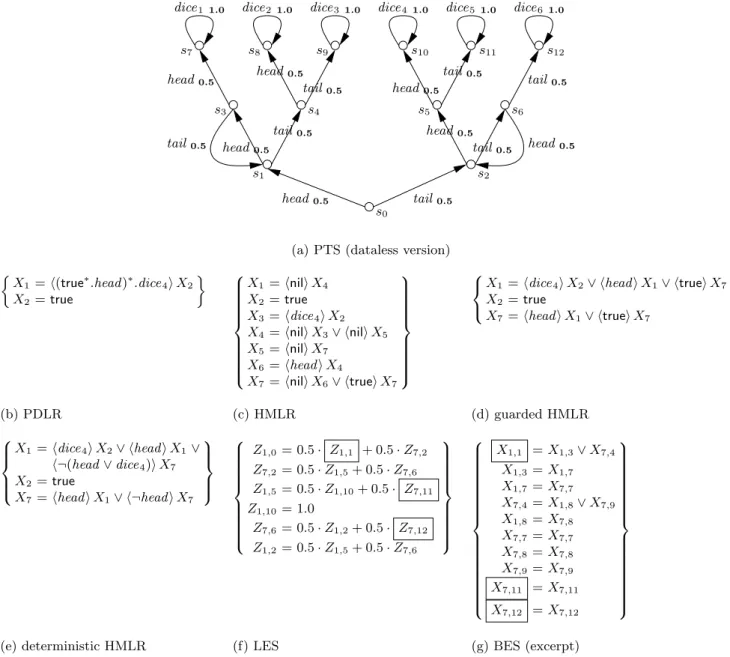
We illustrate the model checking method using the classical example of a six-sided dice emulated using a fair coin [33]. First, we consider a dataless version of the system (i.e., in which actions are simply names), repre-sented as a PTS in Figure 2(a). The actions of tossing a head or tail of the coin are denoted byhead and tail, each one having 0.5 probability. The actions correspond-ing to the dice faces are denoted bydicei for 1≤i≤6, each one occurring with probability 1. We will check on this PTS the formulaΨ1, stating that the probability of
reaching the dice side marked with four directly after tossing the last head (if any) is at least 1/6:
Ψ1={(true∗.head)∗.dice4}≥0.16
Strictly speaking, this formula could be verified us-ing a PACTL model checker, since the regular sub-formula can be expressed equivalently without nested star operators as dice4|(true∗.head.dice
4). The
exis-tence of a path matching it can be specified in ACTL using two Until operators:E[truefalseUdice4 true]∨
E[truetrue Uhead E[truefalse Udice4 true]]. This would
re-quire the model checker to compute the probability mea-sures of each Until operator, then check that their sum is at least 0.16. However, we use formulaΨ1 for the sake
of simplicity to illustrate our model checking procedure. Examples of more complex properties, most of them un-expressible in PACTL, can be found in Section 6. 1. Translation to PDL with recursion. To evaluate an operator {β}≥p on a PTS M = S, A, T,P, si on the fly, one needs to determine the set of paths going out of si and satisfyingβ, to compute the probability measure of this set, and to compare it withp. For this purpose, it is more appropriate to use an equational representation of β, namely PDLR (PDL with recursion), which was introduced in [47] for model checking PDL formulas. A PDLR specification is a system of fixed point equations having propositional variablesX ∈ X in their left hand side and PDL formulasϕin their right hand side:
{Xi=ϕi}1≤i≤n
where ϕi are modal state formulas (see Fig. 1) and X1
is the variable of interest corresponding to the desired property. Since formulasϕimay be open (i.e., contain oc-currences of variablesXj), their interpretation is defined w.r.t. a propositional contextρ:X →2S, which assigns state sets to all variables occurring in ϕi. The interpre-tation of a PDLR specification is the value ofX1 in the
least fixed pointµΦof the functionalΦ: (2S)n→(2S)n defined by:
Φ(U1, ..., Un) =h[[ϕi]]ρ[U1/X1, ..., Un/Xn]i1≤i≤n
where [[ϕi]]ρ= {s ∈ S | s |=ρ ϕi}, and the interpreta-tion ofϕi (see Fig. 1) is extended with the rule “s|=ρ X iff s ∈ ρ(X)”. The notation ρ[U1/X1, ..., Un/Xn] stands for the contextρin whichXi were assignedUi.
In the sequel, we consider PDLR specifications in derivative normal form (RNF), which are the modal logic counterparts of Brzozowski’s (generalized) deriva-tives of regular expressions [10]:
n
Xi=Wni
j=1(ϕij∧ hβijiXij)∨ϕi
o
1≤i≤n
where ϕij and ϕi are closed state formulas. Note that, in the right hand side of equation i, the same variable Xij ∈ {X1, ..., Xn} may occur several times in the first
disjunct. Intuitively, a variable Xi denotes the set of states from which there exists a path with a prefix sat-isfying some of the regular formulas βij and whose last state satisfies Xij. This is formalized using path pred-icates Pi : PathsM → bool, defined by the following system of equations: Pi(σ) =W ni j=1∃lij ≥0.(σ[0]|=ϕij ∧ σ[0, lij]|=βij∧Pij(σlij)) ∨ σ[0]|=ϕi 1≤i≤n
More precisely, (µΦ)i={s∈S| ∃σ∈PathsM(s).Pi(σ)}. The PDLR specification in RNF associated to a for-mulaβ is defined below:
{X1=hβiX2 X2=true}
in which the variable of interest X1 denotes the PDL
formulahβitrue, expressing the existence of a path with a prefix satisfyingβ and leading to some final state de-noted byX2. The corresponding path predicates are: {P1(σ) =∃l≥0.(σ[0, l]|=β∧P2(σl)) P2(σ) =true}
According to the interpretation of regular formulas (see Fig. 1), the path predicateP1(σ) holds iff σ |= β, and
also (µΦ)1={s∈S| ∃σ∈PathsM(s).σ|=β}.
2. Translation to HML with recursion. To bring the PDLR specification closer to an equation system suit-able for verification, one must simplify it by removing the regular operators occurring in modalities. This yields a HMLR (HML with recursion) specification [38], which contains only HML modalities on action formulas. Regu-lar operators can be eliminated by applying the following substitutions, which are valid equalities in PDL [24]:
hϕ?iX =ϕ∧ hniliX
hβ1.β2iX =hβ1iX0 whereX0=hβ2iX hβ1|β2iX =hβ1iX∨ hβ2iX
hβ∗iX =hniliX0 whereX0 =hniliX∨ hβiX0 The rules for the ‘.’ and ‘*’ operators create new equa-tions, necessary for maintaining the PDLR specification in RNF (the insertion of hniliX modalities, which are
s0 s3 s4 s5 s6 s7 s8 s9 s10 s11 s12 dice6 1.0 dice4 1.0 head0.5 tail0.5 head0.5 s2 s1 head0.5 tail0.5 tail0.5 tail0.5 head0.5 tail0.5 dice1 1.0 dice2 1.0 dice3 1.0 dice5 1.0
head0.5 tail0.5
head0.5 tail0.5 head
0.5
(a) PTS (dataless version)
X1 =h(true∗.head)∗.dice4iX2 X2 =true X1 =hniliX4 X2 =true X3 =hdice4iX2 X4 =hniliX3∨ hniliX5 X5 =hniliX7 X6 =hheadiX4 X7 =hniliX6∨ htrueiX7
X1 =hdice4iX2∨ hheadiX1∨ htrueiX7 X2 =true X7 =hheadiX1∨ htrueiX7 (b) PDLR (c) HMLR (d) guarded HMLR X1 =hdice4iX2∨ hheadiX1∨ h¬(head∨dice4)iX7 X2 =true X7 =hheadiX1∨ h¬headiX7 Z1,0 = 0.5· Z1,1 + 0.5·Z7,2 Z7,2 = 0.5·Z1,5+ 0.5·Z7,6 Z1,5 = 0.5·Z1,10+ 0.5· Z7,11 Z1,10= 1.0 Z7,6 = 0.5·Z1,2+ 0.5· Z7,12 Z1,2 = 0.5·Z1,5+ 0.5·Z7,6 X1,1 =X1,3∨X7,4 X1,3=X1,7 X1,7=X7,7 X7,4=X1,8∨X7,9 X1,8=X7,8 X7,7=X7,7 X7,8=X7,8 X7,9=X7,9 X7,11 =X7,11 X7,12 =X7,12
(e) deterministic HMLR (f) LES (g) BES (excerpt)
Fig. 2: Model checking formulaΨ1={(true∗.head)∗.dice4}≥0.16on the PTS simulating the six-sided dice using a coin
equivalent to X, serves the same purpose). The rule for the ‘|’ operator creates two occurrences of the same vari-able X, reflecting that a same state can be reached by two different paths. These rules preserve the path pred-icates Pi associated to the PDLR specification, and in particular P1(σ), which specifies that a pathσ satisfies
the initial formulaβ.
The size of the resulting HMLR specification (num-ber of variables and operators) is linear w.r.t. the size ofβ(number of operators and action formulas). Besides pure HML modalities, the HMLR specification may also contain occurrences of hniliX modalities, which will be eliminated in the next step.
3. Transformation to guarded form. The right hand side of an equationiof the HMLR specification may contain
modalities of the formhαijiXijandhniliXij (equivalent toXij), which correspond toguarded andunguarded oc-currences of variablesXij, respectively. To facilitate the formulation of the verification problem in terms of equa-tion systems, it is useful to remove unguarded occur-rences of variables. The general procedure for transform-ing arbitrary µ-calculus formulas to guarded form [34] can be specialized for HMLR specifications by applying the following actions for each equation definingXi:
– Remove the unguarded occurrences ofXiin the right hand side of the equation defining Xi by replac-ing them with false, which amounts to apply the µ-calculus equalityµX.(X∨ϕ) =µX.ϕ.
– Substitute all unguarded occurrences of Xi in other equations with the right hand side formula of
equa-tioni, and rearrange the right hand sides to maintain the equations in RNF.
This produces a guarded HMLR specification: n Xi=W ni j=1(ϕij∧ hαijiXij)∨ϕi o 1≤i≤n
which is the exact modal logic counterpart of Brzo-zowski’s derivatives of regular expressions [10] defined on the alphabet of action formulas. The transformation to guarded form generally decreases the number of equa-tions in the HMLR specification (by producing unreach-able and/or duplicate equations, which are eliminated), but may increase the number of operators in the right hand sides.
4. Determinization. A guarded HMLR specification may contain, in the right hand side of an equationi, sev-eralalternatives ϕij∧ hαijiXij whose guardsϕij and/or action formulasαij are not disjoint, i.e., they can match the same transition going out of the current state. This is a form of nondeterminism, meaning that the same tran-sitions→a s0can start a pathσsatisfying the path pred-icatePi(σ) in several ways, corresponding to alternative suffixes of the initial regular formulaβ. To ensure a cor-rect translation of the verification problem into a LES, it is necessary to determinize the equations. This can be done by applying the classical subset construction, which produces a deterministic HMLR specification defined on meta-variables (i.e., sets of propositional variables):
XI =W ∅⊂J⊆alt(I) W ∅⊂L⊆J V ij∈Jϕij∧Vi0j0∈alt(I)\J¬ϕi0j0 ∧ V kl∈Lαkl∧ V k0l0∈J\L¬αk0l0XL ∨ W i∈Iϕi I⊆[1,n]
where I ⊆ [1, n] is a subset of the variable indices and XI is a shorthand notation for the meta-variable
{Xi | i∈I}. Given a subsetI, the set of indices of al-ternatives contained in the equations defining variables in XI is alt(I) ={ij |i ∈I∧j ∈[1, ni]}. A transition s→a s0 matches an alternativeϕij∧ hαijiXij ifs|=ϕij, a |=αij, and s0 |=Xij. Intuitively, the right hand side of the meta-equation definingXI is obtained by consid-ering all situations when a transitions→a s0 matches a subset of the alternatives alt(I) and requiring that the target states0satisfies the meta-variable induced by the matching alternatives. For a transitions→a s0 to match a subset of alternatives J ⊆ alt(I), state s must sat-isfy all guardsϕij of alternatives in J, and none of the guards of alternatives inalt(I)\J. Then, for all modal-itieshαijiXij contained in the alternatives inJ, it may be the case thatasatisfies only the action formulas con-tained in a subsetL⊆J of alternatives (and none of the action formulas of the alternatives inJ\L), and therefore
s0 must satisfy the meta-variable XL. As shown in [44] for a similar construction in the state-based setting, the determinization preserves the path predicate associated to the variables of interest X1 and X{1} in the HMLR before and after determinization, i.e., P1(σ) = P{1}(σ) for any pathσ∈PathsM.
In the worst case, determinization may yield an ex-ponential increase in the size of the HMLR specification. However, this happens on pathological examples of reg-ular formulas, which rarely occur in practice; most of the time, the nondeterminism contained in a formula β is caused by a lack of precision regarding the itera-tion operators, which can be corrected by constraining the action formulas corresponding to iteration “exits”. For example, the regular formula contained in Ψ1 can
be made deterministic by specifying precisely that the occurrences of thehead action are separated by actions other thanhead and by taking into account that, in the PTS of Figure 2(a), a dice action cannot occur before a head: ((¬head)∗.head)∗.dice4. In practice, the size of
the determinized HMLR specification can be reduced by eliminating duplicate equations and by identifying con-tradictory combinations and absorptions of action for-mulas (α1∧α2=falseandα1∧ ¬α2 =α1 whenα1, α2
are disjoint).
5. Translation to linear and Boolean equation systems. Consider a determinized HMLR specification in RNF (in which the meta-variables have been renamed into ordi-nary propositional variables) corresponding to a regular formulaβ:
n
Xi=Wni
j=1(ϕij∧ hαijiXij)∨ϕi
o
1≤i≤n
whereαij∧αik=falsefor eachi∈[1, n] andj, k∈[1, ni] withj 6=k. The associated path predicates are defined as follows: Pi(σ) =W ni j=1(σ[0]|=ϕij∧σa[0]|=αij ∧ Pij(σ1)) ∨ σ[0]|=ϕi 1≤i≤n
They are related to the HMLR specification by (µΦ)i=
{s∈S | ∃σ∈PathsM(s).Pi(σ)}, and to the initial regu-lar formulaβ byP1(σ) =σ|=β.
The last step of the model checking method reformu-lates the problem of verifying the determinized HMLR specification on a PTS in terms of solving a LES (∗) and a BES (∗∗) defined as follows:
Zi,s =if s6|=Xi then 0 else ifs|=ϕi then1 else ni X j=1 if s6|=ϕij then 0 else X s→a s0 a|=αij P(s, a, s0)·Zij,s0 1≤i≤n s∈S (∗) Xi,s =Wni j=1 s|=ϕij ∧ W s→sa 0 a|=αij∧Xij,s0 ∨ s|=ϕi 1≤i≤n s∈S (∗∗)
The LES (∗) is obtained by a translation similar to the classical one defined originally for PCTL [29]. A nu-merical variableZi,s denotes the probability measure of the paths going out of state s and satisfying the path predicate Pi. The BES (∗∗), with minimal fixed point semantics, is produced by the classical translation em-ployed for model checking modalµ-calculus formulas on LTSs [16, 3]. A Boolean variable Xi,s is true iff state s satisfies the propositional variable Xi of the HMLR specification. The on-the-fly model checking consists in solving the variable Z1,si, which denotes the probabil-ity measure of the set of paths going out of the initial statesi of the PTS and satisfying the initial regular for-mula β. This is carried out using local LES and BES resolution algorithms, as will be explained in Section 5. The conditionss|=Xi occurring in the LES (∗) and the conditions s |=ϕij, s|= ϕi occurring in both equation systems are checked by applying the on-the-fly model checking method for solving the variableXs
i of the BES (∗∗) and for evaluating the closed state formulasϕij, ϕi on state s.
The determinization of the HMLR specification guar-antees that the sum of coefficients in the right hand side of each equation of the LES is at most 1. If the HMLR specification is not determinized, such as the one shown in Figure 3(c), the LES encoding the interpretation of the formula on the PTS in Figure 3(a) has the wrong solution Z1,0 = 2.0 (variable Z1,2 = 0 since s2 6|= X1,
and variables Z2,1 = Z2,2 = 1 since X2 = true). This
is because the nondeterministic equation definingX1in
the HMLR specification matches twice the suffix of the path going out ofs0. Note that determinization ensures
a sound LES translation also if some states have several outgoing transitions labeled by the same action a.
The condition s 6|= Xi surrounded in the LES (*) has the role of pruning the exploration of the PTS if the current statesdoes not have any outgoing path match-ing the suffix of β denoted by Xi. As explained in [7, Chap. 10], this is necessary to avoid singularities in the
a1.0 a1.0 b1.0 s0 s1 s2 X1 =haiX2∨ htrueiX1 X2 =true (a) PTS (c) guarded HMLR {true∗.a}≥0 ( Z1,0 = 1.0·Z2,1+ 1.0·Z1,1 Z1,1 = 1.0·Z2,2+ 1.0· Z1,2 ) (b) formula (d) LES
Fig. 3: Nondeterministic regular formula
a0.5 s0 s1 c1.0 b0.5 X1 =haiX2∨ h¬aiX1 X2 =true (a) PTS (c) deterministic HMLR {(¬a)∗.a}≥0 Z1,0 = 0.5·Z2,0+ 0.5·Z1,1 Z1,1 = 1.0·Z1,1 (b) formula (d) LES
Fig. 4: Unreachable path suffix
LES and ensure a unique solution. For example, if we neglect the condition s6|=Xi when checking the deter-ministic HMLR specification shown in Figure 4(c) on the PTS shown in Figure 4(a), the resulting LES con-tains the singular equationZ1,1=Z1,1. This is precisely
becauses16|=X1, meaning that froms1there is no path
matching the regular formula suffix denoted byX1.
By solving the LES obtained in Figure 2(f), we ob-tain Z1,0 = 1/6, meaning that tossing the head of the
coin an (arbitrarily large) number of times corresponds to rolling the four-side of the dice with 1/6 probability, and therefore the formula Ψ1 is valid on the PTS. The
numerical variablesZ1,1,Z7,11, andZ7,12surrounded by
boxes in Figure 2(f) are equal to 0, since the path suf-fixes denoted by the propositional variablesX1 andX7
are not reachable from statess1,s11, ands12of the PTS;
this is checked by solving the Boolean variables X1,1,
X7,11, and X7,12 of the BES in Figure 2(g), which are
equal to false. If we evaluate the Ψ1 formula for every
dicei action, we obtain a probability equal to 1/6 for i∈ {1,2,4} and to 0 fori∈ {3,5,6}, the latter sides of the dice being not directly reachable after aheadaction.
4 Extension with data handling
The regular formulas that we used so far belong to the dataless fragment [47] of MCL, which considers actions
simply as names of communication channels. In practice, the analysis of value-passing concurrent systems, whose actions typically consist of channel names and data val-ues, requires the ability to extract and manipulate these elements. For this purpose, MCL [48] provides action predicates extracting and/or matching data values, regu-lar formulas involving data variables, and parameterized fixed point operators. The regular probabilistic operator
{β}≥pcan be naturally extended with the data handling regular formulas of MCL, which enable to characterize complex paths in a PTS modeling a value-passing con-current system.
To improve versatility, we extend the regular formu-las of MCL with a general iteration operator “loop”, which subsumes the classical regular operators with counters, and can also specify paths having a certain cost calculated from the data values carried by its ac-tions. After briefly recalling the main data handling op-erators of MCL, we define the “loop” operator, illustrate its expressiveness, and show how the on-the-fly model checking procedure previously described is generalized to deal with the data handling probabilistic operator.
4.1 Overview of data handling MCL operators
In the PTSs modeling value-passing systems, actions are of the form “c v1. . . vn”, wherecis a channel name and v1, ..., vn are the data values exchanged during the ren-dezvous on c. To handle the data values contained in actions, MCL provides several basic constructs, defined in Figure 5. Data expressionseare built over data vari-ables xand functions f (restricted, for simplicity, to a single argument in Fig. 5). The interpretation ofeis de-fined w.r.t. a data contextδassigning values to all data variables occurring ine.
Actions containing data are specified using action predicates of the form “{c !e}” (value matching) or “{c ?x:T}” (value extraction). The former predicate matches an action c v with v equal to the value of e, whereas the latter predicate also captures the value v (which must be of type T) and stores it in the variable x. The successful evaluation of a predicate “{c?x:T}” on an actionaalso produces a data contextenva({c?x:T}) wherexis assigned the value extracted froma. The ac-tion predicates of MCL are slightly more involved than those shown in Figure 5: several clauses “!e” and “?x:T” can be freely combined (the variables defined in the ex-traction clauses are visible inside the action predicate and also in the enclosing formula), the “...” wildcard can be used to match zero or more values, and an op-tional clause “whereb” can be used to specify a Boolean conditionb over the extracted variables. An action sat-isfies an action predicate if its structure is compatible with the clauses of the predicate and the “where” guard (if present) evaluates to true in the context of the data variables extracted from that action.
Expressions: e::=x|f(e) [[x]]δ = δ(x) [[f(e)]]δ = f([[e]]δ) Action patterns: α::={c!e} | {c?x:T} [[{c!e}]]δ = {c [[e]]δ} [[{c?x:T}]]δ = {c v|v∈T} envc v({c?x:T}) = [v/x] ifv∈T enva(α) = [ ] otherwise State formulas: ϕ::=hαiϕ|Y(e)|µY(x:T:=e).ϕ [[hαiϕ]]ρδ = {s∈S| ∃s→a s0.a∈[[α]]δ∧ s0∈[[ϕ]]ρ(δenva(α))} [[Y(e)]]ρδ = ρ(Y)([[e]]δ) [[µY(x:T:=e).ϕ]]ρδ = µΦρδ([[e]]δ) whereΦρδ: (T→2S)→(T →2S), (Φρδ(F))(v) = [[ϕ]] (ρ[F/Y])(δ[v/x])
Fig. 5: Syntax and semantics of basic MCL operators
The basic state formulas of MCL are built from Boolean connectors, modalities, and parameterized fixed point operators (restricted, for simplicity, to a single pa-rameter in Fig. 5). A fixed point formulaµY(x:T:=e).ϕ denotes both the definition and the call in situ of a propositional variable Y parameterized by x. Its inter-pretation w.r.t. a propositional contextρand a data con-textδis the call ofµΦρδ with the value ofein the con-textδ,µΦρδ being the minimal solution of the equation Y(x) =ϕinterpreted w.r.t. the contextsρandδ.
Regular formulas in MCL are built over action pred-icates using the classical operators shown in Section 2, as well as constructs inspired from sequential program-ming languages: conditional (“if-then-else”), counting, it-eration (“for” and “loop”, described in Subsection 4.2), and definition of variables (“let”). Finally, the state for-mulas of MCL also provide modalities containing regular formulas, quantifiers over finite domains, and program-ming language constructs (“if” and “let”) [48].
4.2 Generalized iteration on regular formulas
The general iteration mechanism that we propose on reg-ular formulas consists of three operators having the fol-lowing syntax: β ::=loop(x:T:=e0) : (x0:T0)in β end loop | continue(e) | exit (e0)
The “loop” operator denotes a path made by concate-nation of (zero or more) path fragments satisfying β, each one corresponding to an iteration of the loop with the current value of variablex. The iteration variablex, which is visible inside the loop bodyβ, is initialized with the value of expressione0 at the first loop iteration and
can be updated to the value ofe by using the operator “continue(e)”, which starts a new iteration of the loop. The loop is terminated by means of the “exit (e0)” op-erator, which sets the return variablex0, visible outside the “loop” formula, to the value ofe0.
The iteration and return variables (xandx0) are both optional; if they are absent, the “in” keyword is also omitted. For simplicity, we used only one variablexand x0, but several variables of each kind are allowed. The ar-guments of the operators “continue” and “exit” invoked in the loop body β must be compatible with the dec-larations of iteration and return variables, respectively. Every occurrence of “continue” and “exit” refers to the immediately enclosing “loop”, which enforces a specifi-cation style similar to structured programming.
For conciseness, we define the semantics of the “loop” operator by translating it to basic MCL in the context of an enclosing diamond modality (a dual translation holds for an enclosing box modality). The translation loop2mclZ/x:T /x0:T0(ϕ) is defined in Figure 6, where x
andx0 are the iteration and return data variables of the immediately enclosing “loop”, andZis the propositional variable associated to it. Basically, a possibility modality enclosing a “loop” operator is translated into a minimal fixed point operator parameterized by the iteration vari-able(s). The occurrences of “continue” in the body of the loop are translated into calls of the propositional vari-able with the corresponding arguments, and the occur-rences of “exit” are translated into “let” state formulas defining the return variables and assigning them the cor-responding return values. The rules for the other regular operators generalize those of the translation from PDL to modalµ-calculus [22].
All iteration operators on MCL regular formulas can be expressed in terms of the “loop” operator, as shown in Table 1. For simplicity, we omitted the definition of β∗, β+, β{e} (iteration e times), and β{... e} (iteration at mostetimes), which are equivalent toβ{0...},β{1...}, β{e ... e}, andβ{0... e}, respectively.
To illustrate the semantics of general iteration, con-sider the formula hβ{e}itrue stating the existence of a path made ofepath fragments satisfyingβ. By encoding bounded iteration as a “loop” and applying the transla-tion rules of general iteratransla-tion, we obtain:
Table 1: Encoding MCL iteration operators using “loop” Syntax Meaning Encoding using “loop” β{e ...} ≥etimes loop(c:nat:=e)in
ifc >0then β .continue(c−1) else exit|β .continue(c) end if end loop
β{e1 ... e2} between loop(c1:nat:=e1, e1ande2 c2:nat:=e2−e1) times in ifc1>0then β .continue(c1−1, c2) elsifc2>0then exit| β .continue(c1, c2−1) else exit end if end loop
forn:nat stepwise loop(n:nat:=e1)in frome1 ifn < e2 then
toe2 β .continue(n+e3)
stepe3 else
do exit
β end if
end for end loop
hβ{e}itrue = * loop(c:nat:=e)in ifc >0 then β .continue(c−1) else exit end if end loop + true = µZ(c:nat:=e). ifc >0then hβiZ(c−1) else true end if
The bounded iteration operatorsβ{e},β{e ...}, and β{e1 ... e2} are natural means for counting actions
(ticks), and hence describing discrete-time properties. The full Until operator of PCTL, and its action-based counterparts derived from ACTL, can be expressed as follows (wheret≥0 is the number of ticks untilϕ2):
ϕ1 U≤t ϕ2≥p={(ϕ1?.true){0... t}.ϕ2?}≥p ϕ1α1 U ≤t ϕ 2 ≥p={(ϕ1?.α1){0... t}.ϕ2?}≥p ϕ1α1 U ≤t α2 ϕ2 ≥p={(ϕ1?.α1){0... t}.ϕ1?.α2.ϕ2?}≥p
loop2mclZ/x:T /x0:T0 *loop(x:T:=e0) : (x0:T0)in β end loop + ϕ def = µY(x:T:=e0).loop2mclY /x:T /x0:T0(hβiϕ) loop2mclZ/x:T /x0:T0(hcontinue(e)iϕ) def = Z(e) loop2mclZ/x:T /x0:T0(hexit(e0)iϕ) def
= letx0:T0:=e0in loop2mclZ/x:T /x0:T0(ϕ)end let
loop2mclZ/x:T /x0:T0(hαiϕ) def = hαiloop2mclZ/x:T /x0:T0(ϕ) loop2mclZ/x:T /x0:T0(hϕ1?iϕ) def = hloop2mclZ/x:T /x0:T0(ϕ1)?iloop2mclZ/x:T /x0:T0(ϕ) loop2mclZ/x:T /x0:T0(hβ1|β2iϕ) def = loop2mclZ/x:T /x0:T0(hβ1iϕ)∨loop2mclZ/x:T /x0:T0(hβ2iϕ) loop2mclZ/x:T /x0:T0(hβ1.β2iϕ) def = loop2mclZ/x:T /x0:T0(hβ1iloop2mclZ/x:T /x0:T0(hβ2iϕ)) loop2mclZ/x:T /x0:T0(hβ∗iϕ) def
= µY.(loop2mclZ/x:T /x0:T0(ϕ)∨loop2mclZ/x:T /x0:T0(hβiY))
Fig. 6: Translation of the general iteration operators in basic MCL
Besides counting, the “loop” operator can characterize complex paths in a PTS, by collecting the data values (costs) present on actions and using them in arbitrary computations, as it will be illustrated in Section 6. 4.3 Model checking method with data handling
The on-the-fly model checking method described in Sec-tion 3 can be generalized to deal with the data handling constructs of MCL by adding data parameters to the various equation systems used as intermediate forms.
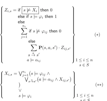
We illustrate the complete method on a data han-dling version of the PTS modeling the six-sided dice us-ing a fair coin, shown on Figure 7(a). The actions of toss-ing the head and tail of the coin are denoted by “toss1” and “toss 0”, and the actions corresponding to the dice faces are denoted by “dicei” for 1≤i≤6. We will check on this PTS the formulaΨ2, stating that the probability
of reaching the dice side marked with one by tossing first a side of the coin and then tossing the same side at most ntimes (wherenis a parameter to be instantiated) is at least 10%:
Ψ2={ {toss ?v:nat}.
((¬{toss !v})∗.{toss !v}){... n}.
{dice !1} }≥0.1
The various translation phases are illustrated on Fig-ure 7. The translation rules for standard regular op-erators given in Section 3, extended with data han-dling, are applied for eliminating the “.” operators in the PDLR specification. To facilitate the subsequent model checking steps, the new equations introduced by these rules are data-closed, i.e., the propositional vari-ables in their left hand sides are parameterized by the
data variables occurring in their right hand side formu-las. For example, when translating the right hand side of the equation definingX1, the extended rule applied
is h{toss ?v:nat}.βiX2 = h{toss ?v:nat}iX3(v), where
X3(v) =hβiX2, ensuring that data variablevoccurring
inβis a parameter ofX3. Then, the iteration at mostn
times is translated into a “loop” operator, and the corre-sponding modality is further refined using the semantics of “loop” defined in Section 4.2, yielding a HMLR speci-fication parameterized by a countercand by the valuev of the coin side captured by the first action of the regular formula (Fig. 7(c)).
This HMLR specification is then brought to guarded form (Fig. 7(d)) by carrying out systematically the ap-propriate substitutions and keeping track of the data parameters. For example, variable X3(v) is replaced
by X5(v, n) in the equation of X1, and X6(v, c) is
re-placed byh{toss !v}iX5(v, c−1) in the equation defining
X7(v, c).
The guarded HMLR specification is deter-minized by ensuring that the alternatives in the right hand side of equation defining X5(v, c) are
mutually exclusive (all the other equations being already deterministic). This produces the alter-natives h{dice !1} ∧ ¬{toss !v}i {X2, X7(v, c)} and h¬{toss !v} ∧ ¬{dice !1}i {X7(v, c)}. The former
al-ternative is equivalent to h{dice !1}i {X2} because
{dice !1} ⇒ ¬{toss !v} and X2 denotes the final states
of the paths satisfying the initial regular formula. The other alternatives present in the equations led to singleton meta-variables, which are replaced by the variables themselves (Fig. 7(e)).
Next, a parameterized LES is produced (Fig. 7(f)) by the translation scheme given in Section 3, extended to handle data parameters. For instance, variableZ5,1(1, n)
in the LES denotes the probability measure of the paths starting from states1 and satisfying the path predicate
denoted byX5with the parametersvandcset to 1 and
n, respectively. The numerical variables Z5,2(0, n) and
Z7,4(1, c) surrounded by boxes in Figure 7(f) are equal
to 0, since the path suffixes denoted by the propositional variables X5(0, n) and X7(1, c) are not reachable from
statess2ands4of the PTS (this is checked by solving the
corresponding Boolean variables of the BES, not shown in Figure 7).
Finally, a plain LES is generated (Fig. 7(g)) by in-stantiatingn= 2 in the parameterized LES. By solving this LES (e.g., using substitution), we obtain Z1,0 =
0.125, which is the probability measure of the paths starting from the initial states0of the PTS and
satisfy-ing the regular formula specified inΨ2. In other words,
tossing first a side of the coin, then tossing again the same side at mostn= 2 times corresponds with 12.5% probability to rolling the one-side of the dice, and there-fore theΨ2 formula is valid on the PTS in Figure 7(a).
If we evaluate the Ψ2 formula withn = 2 for every
ac-tion “dice i”, we obtain a probability equal to 0.125 for i∈ {1,6}, to 0.156 fori∈ {2,5}, and to 0 fori∈ {3,4}, the latter sides of the dice being not reachable after toss-ing once, then at mostn= 2 times the same side of the coin.
4.4 Soundness and termination of the method
The presence of data parameters (with infinite domains) in the regular formulas β makes necessary two addi-tional hypotheses about the structure of β in order to ensure the feasibility of our model checking method for the probabilistic operator{β}≥p.
Soundness of the translation to guarded form. The translation of (parameterized) HMLR specifications to guarded form relies on the absorption property for µ-calculus formulas with data parameters:
µX(u).(X(u)∨ϕ) =µX(u).ϕ
where ϕ may contain occurrences of the propositional variable X with arbitrary data arguments. The above equality does not hold anymore if the unguarded oc-currence of X in the left hand side has an argument e different from the parameteru. Typically, such cases cor-respond to regular formulas that perform pure compu-tations on data without exploring any transition in the PTS. For example, the following regular modality spec-ifies the classical primality testing of a natural number n (odd and greater than 3) by checking that n is not
divided by any of the odd numbers from 3 to√n:
hloop(k:nat:=3) : (r:bool)in ifk∗k > nthen exit(true) elsifn%k= 0then exit(false) else continue(k+ 2) end if end loopir
The corresponding HMLR specification, shown below, contains the unguarded occurrenceX2(k+2), which
can-not be eliminated by absorption: X1=X2(3) X2(k) =ifk∗k > n then true elsifn%k= 0then false else X2(k+ 2) end if
In practice, we forbid such kind of regular formulas purely operating on data, since they can be replaced by functions, and we reserve regular formulas for the spec-ification of (non empty) paths in the PTS.
Termination of the LES and BES construction. After translating the regular formula into a (parameterized) deterministic HMLR specification, the last phase of the model checking procedure consists in generating and solving on the fly the LES and BES. These systems de-pend not only on the (finite) information contained in the PTS, but also on the values of the data parame-ters (with infinite domains) created during instantiation. Therefore, the convergence of the whole procedure re-lies on the termination of the instantiation phase, which must create finite LES and BES. This is in general un-decidable, similarly to the termination of term rewrit-ing [19]. Typically, such situations happen for “patholog-ical” formulas, which carry on divergent computations unrelated to the data values contained in the PTS ac-tions. For example, the following modality:
hloop(k:nat:=0)in a .continue(k+ 1) end loopitrue
will not converge on the PTS consisting of a single loop sa→1.0s, since it will entail the construction of an infinite LES {Zs(0) = Zs(1), Zs(1) = Zs(2), ...}. In practice, for such divergent formulas, the instantiation phase will attempt to generate an infinite LES, eventually causing the whole model checking procedure to abort when the available memory is exhausted.
The regular formulasβ used in the probabilistic op-erator are meant to characterizefinite paths in the PTS.
s0
s3 s4 s5 s6
s7 s8 s9 s10 s11 s12
toss00.5 toss10.5
dice21.0 dice51.0 dice61.0 dice11.0 dice31.0 dice41.0
toss10.5 toss00.5 toss10.5 toss00.5 toss10.5 s2 s1 toss10.5 toss10.5 toss00.5 toss00.5 toss10.5 toss00.5 toss00.5
(a) PTS (data handling version)
X1 =h{toss ?v:nat}. ((¬{toss !v})∗. {toss!v}){... n}. {dice !1}iX2 X2 =true X1 =h{toss?v:nat}iX3(v) X2 =true X3(v) =hniliX5(v, n) X4 =h{dice!1}iX2 X5(v, c) =ifc >0then hniliX4∨ hniliX7(v, c) else hniliX4 end if X6(v, c) =h{toss!v}iX5(v, c−1) X7(v, c) =hniliX6(v, c)∨ h¬{toss!v}iX7(v, c) X1 =h{toss?v:nat}iX5(v, n) X2 =true X5(v, c) =ifc >0then h{dice !1}iX2∨ h{toss!v}iX5(v, c−1)∨ h¬{toss!v}iX7(v, c) else h{dice !1}iX2 end if X7(v, c) =h{toss!v}iX5(v, c−1)∨ h¬{toss !v}iX7(v, c) (b) PDLR (c) HMLR (d) guarded HMLR X1 =h{toss ?v:nat}iX5(v, n) X2 =true X5(v, c) =ifc >0then h{dice !1}iX2∨ h{toss !v}iX5(v, c−1)∨ h¬{toss!v} ∧ ¬{dice !1}iX7(v, c) else h{dice !1}iX2 end if X7(v, c) =h{toss !v}iX5(v, c−1)∨ h¬{toss!v}iX7(v, c) Z1,0 = 0.5·Z5,1(1, n) + 0.5· Z5,2(0, n) Z5,1(1, c) =ifc >0then 0.5·Z5,3(1, c−1) + 0.5· Z7,4(1, c) else 0 end if Z5,3(1, c) =ifc >0then 0.5·Z5,7(1, c−1) + 0.5·Z7,1(1, c) else 0 end if Z5,7(1, c) =ifc >0then1 else1end if Z7,1(1, c) = 0.5·Z5,3(1, c−1) + 0.5· Z7,4(1, c) Z1,0 = 0.5·Z5,1(1,2) Z5,1(1,2) = 0.5·Z5,3(1,1) Z5,3(1,1) = 0.5 + 0.5·Z5,3(1,0) Z5,3(1,0) = 0
(e) deterministic HMLR (f) LES (partially instantiated) (g) LES (instantiated forn= 2) Fig. 7: Model checking formulaΨ2={{toss ?v:nat}.((¬{toss !v})∗.{toss !v}){... n}.{dice !1}}≥0.1 on a PTS
Ensuring this becomes undecidable in the presence of the generalized iteration operator “loop”, which enables the specification of arbitrary (Turing computable) paths in a PTS. However, the model checking procedure termi-nates for most practical cases of data handling regular formulas denoting finite paths (counting, accumulating or aggregating values, computing costs over paths).
5 Tool support
We implemented the on-the-fly model checking method described in Sections 3 and 4 within the CADP tool-box [27]. We briefly present here the extension of the ex-isting on-the-fly model checker of MCL with the regular probabilistic operator, and the representations of PTS and DTMC models suitable for probabilistic analysis. Extension of MCL and its model checker. We extended MCL with the general iteration operator “loop” on regular formulas and the regular probabilistic opera-tor {β}./ p, where ./ ∈ {<,≤, >,≥,=}. Temporal and probabilistic operators can be freely combined, e.g., [β1]{β2}≥p specifies that, from all states reached after a path satisfyingβ1, the probability measure of an
out-going path satisfying β2 is at least p. Also, using the
MCL quantifiers on finite data domains, one can suc-cinctly describe data handling probabilistic properties, such as the fact that after zero or more coin tosses, each side of the dice is reached with 1/6 probability: foralli:nat among{1...6}.{ {toss ...}∗.{dice !i} }
≥1/6.
We also enhanced the EVALUATOR [48] on-the-fly model checker with the translation of {β}./ p formulas into BESs (for checking the existence of path suffixes) and LESs (for computing probability measures) as de-scribed in Sections 3 and 4. The on-the-fly resolution of BESs is carried out by the algorithms of the CAE-SAR SOLVE library [43], which already serves as veri-fication back-end for (non-probabilistic) MCL formulas. The resolution algorithms work in a systolic manner: sev-eral subsequent invocations of an algorithm for solving different variables of a BES have a linear overall com-plexity in the size of the BES (number of variables and operators), obtained by keeping the values of all vari-ables computed during intermediate resolutions.
For the on-the-fly resolution of LESs, we designed a local algorithm operating on the associated Signal Flow Graphs (SFG) [12], in a way similar to the BES resolution algorithms, which operate on the associated Boolean graphs [3]. Figure 8 illustrates the SFG of the LES corresponding to the evaluation of property Ψ1 on
the PTS of the six-sided dice, shown in Figure 2(f). In the SFG, each vertex corresponds to a variable of the LES and each edge Zi,s
q
→ Zj,r denotes a dependency ofZi,s uponZj,r, i.e., the fact that the termq·Zj,r oc-curs in the right hand side of the equation definingZi,s (e.g., edges Z1,0
0.5
→Z1,1 andZ1,0 0.5
→ Z7,2 represent the
equationZ1,0= 0.5·Z1,1+ 0.5·Z7,2). Constants are
rep-resented as sink vertices (e.g.,Z1,1 or Z1,10). Self-loops
Zi,s q
→ Zi,s are deleted during the construction of the SFG by updating the coefficients on the edges going out ofZi,s (an edgeZi,sq→ij Zj,r becomes Zi,sqij/→(1−q)Zj,r). The on-the-fly LES resolution algorithm carries out a forward DFS (depth-first search) exploration of the SFG with detection of SCCs (strongly connected com-ponents), starting at the vertex of interest. The SFG is constructed on demand in the following way. For each vertex Zi,s, the BES solver is invoked on the Boolean variable Xi,s to determine whether s has an outgoing sequence matching the suffix of the regular formula β denoted by the propositional variable Xi of the deter-minized HMLR specification (see Fig. 2(e)). If variable Xi,sis false, the vertexZi,sdenotes a constant 0, like the boxed verticesZ1,1, Z7,11, andZ7,12 in Figure 8. When
a constant vertexZj,r is encountered, its value is prop-agated backwards to its predecessor vertexZi,s on the DFS stack, which amounts to perform the substitution of Zj,r in the right-hand side of the equation defining Zi,s. If the vertexZi,s on top of the stack becomes sta-ble(i.e., the values of all its successor vertices have been computed), its value is stored for possible later reuse and is propagated backwards as ifZi,s was a constant.
If variableXi,sis true, then the SFG edges going out ofZi,sare constructed by scanning the right hand side of the corresponding equation in the LES, and the DFS ex-ploration can proceed further. When a non-trivial SCC (i.e., containing at least two vertices) is encountered, the corresponding LES fragment induced by the vertices of the SCC is solved using either Gaussian elimination (for LES fragments with less than 1,000 variables) or the Gauss-Seidel iterative method (for larger LES frag-ments). For the SFG in Figure 8, the DFS traversal will propagate backwards the values of vertices Z1,1, Z1,10,
and Z7,11, stabilizing the vertex Z1,5 at 0.5. Then,
af-ter propagating backwards the vertex Z7,12, the SCC {Z7,6, Z1,2} is detected and solved, stabilizing the ver-ticesZ7,6 andZ1,2 at 1/6 and 1/3, respectively. Finally,
vertex Z7,6 is propagated and stabilizes vertex Z7,2 at
1/3, and then the vertex of interestZ1,0at 1/6.
For the acyclic parts of the SFG, this algorithm amounts to a resolution by substitution, and stores in memory only the vertices (corresponding to LES variables). For each non-trivial SCC, the algorithm stores the vertices and the edges (corresponding to the operands in the right-hand sides of the LES equations) until the SCC has been solved. Therefore, the peak mem-ory consumption is determined by the largest SCC con-tained in the SFG. In practice, it is often the case that the evaluation of probabilistic operators on PTSs pro-duces LESs with SFGs that are not strongly connected (this is the case, e.g., for the SFG in Figure 8 and also for all properties shown in Section 6). In these situa-tions, the SFG-based on-the-fly LES resolution can be
0.0 0.5 0.5 Z1,1 0.0 Z7,11 0.5 0.5 Z1,5 0.5 0.5 0.5 0.5 0.5 1.0 Z1,2 Z7,12 0.0 SCC 0.5 Z1,10 Z1,0 Z7,2 Z7,6
Fig. 8: Signal Flow Graph of the LES in Figure 2(f)
less memory consuming than a global resolution work-ing on the entirely constructed LES.
Representation of PTSs. The concurrent systems under analysis in CADP are described formally using the LNT language [11], inspired from value-passing process alge-bras and classical programming languages. An LNT de-scription is compiled into an LTS represented implic-itly as a C program implementing the successor function according to the OPEN/CAESAR application program-ming interface [25] for on-the-fly graph exploration. This LTS is converted on the fly into a PTS by adding prob-abilities to its actions (transition labels) using the label renaming feature of EVALUATOR. By default, all tran-sitions going out of a state are equiprobable, in which case there is no need to specify any probability distri-bution (this happens, e.g., for the PTSs modeling the dice, shown in Fig. 2(a) and 7(a)). If one assigns a spe-cific probabilitypto some action a, then for each state s having an outgoing transition s →a s0, the remaining probability 1−p is equally distributed on the actions labeling the neighbour transitions s →b s0. In this way, an LNT description can be converted on the fly (with-out any additional annotation) into a PTS during the verification of a probabilistic MCL formula.
Representation of DTMCs. Although the modeling and verification approach of CADP is action-based, the un-derlying models can be adapted to accomodate for state-based analysis, by encoding the relevant information on actions instead of states. Thus, a DTMC having atomic propositions on states can be converted into a PTS by “pushing” all state information on the actions labeling the outgoing transitions. For example, if a set of atomic propositions q1, ..., qn hold on a state s of a DTMC,
then the transitions going out of sin the corresponding PTS will be labeled by actions of the form “A q1. . . qn”
and will keep the same probabilities as in the DTMC. This scheme, which does not change the structure of the graph, relies on the data handling modalities of MCL
for expressing atomic propositions on states: a state sat-isfying qi in the DTMC satisfies the diamond modality
h{A?any...?any!qi ...}itruein the PTS, where “?any” is a wildcard matching a value of any type. Using the macro-definition mechanism of MCL, the atomic propo-sitions can be encoded as macros with symbolic names and reused in state-based formulas.
In this way, one can check state-based proper-ties using the PCTL operators encoded in terms of
{β}≥p as shown in Section 4.2. Moreover, the reg-ular operators of MCL enable one to specify prop-erties more expressive than Until operators, such as
{send?.true.(retry?.true∗)∗.recv?}
≥0.9, where the atomic
propositions like send are macro-definition names for the modalitiesh{A!send}itrueand they are checked on states using the testing operator “?” of PDL.
6 Case studies
We illustrate the application of the regular probabilis-tic operator by carrying out a probabilisprobabilis-tic analysis of several concurrent systems. First, we consider several shared-memory mutual exclusion protocols (Sec. 6.1), and corroborate the results of the probabilistic analysis with those previously obtained by a steady-state analy-sis using CTMCs in [46]. Then, we compare our on-the-fly model checker procedure with the explicit-state algo-rithms of the probabilistic model checker PRISM [36], by analyzing the Bounded Retransmission Protocol (Sec. 6.2) and two randomized protocols (Sec. 6.3). All model checking experiments have been carried out on a single core of an Intel(R) Xeon(R) E5-2630v3 @2.4GHz with 128 GBytes of RAM and Linux Debian 7.9 within a cluster of Grid’5000 [9].
We considered the explicit-state engine of PRISM in order to achieve a consistent comparison with our on-the-fly verification algorithms, which operate on explicit-state PTSs; however, some of the performance figures re-ported below (e.g., in Sec. 6.2) are close to those of the PRISM benchmarks1, which were conducted using the
symbolic engine of PRISM. The time and memory con-sumption measured for the two tools include the time of constructing the model (i.e., launching the Java virtual machine and building the DTMC by PRISM, compil-ing the LNT description and convertcompil-ing the state space on the fly into a PTS by CADP). Given that PRISM and CADP are very different in their architecture, algo-rithms, and implementation, the experimental measures presented in this section are not meant to provide an absolutely precise comparison of the tools performance, but rather to give general tendencies for various sizes of the models considered.
6.1 Mutual exclusion protocols
We focus here on a subset of the 27 protocols speci-fied in LNT and studied in [46], namely the CLH, MCS, Burns&Lynch (BL), Lamport, Peterson, TAS and TTAS protocols, by considering configurations of N ≤5 con-current processes competing to access the critical sec-tion. Each process executes cyclically a sequence of four sections: non critical, entry, critical, and exit. The en-try and exit sections represent the algorithm specific to each protocol for demanding and releasing the access to the critical section, respectively. During these sections, each protocol carries out various operations (read, write, test-and-set, etc.) on the shared variables.
In the PTS models of the protocols, all transitions going out of each state have equal probabilities, mean-ing that each process has the same chances to execute. This kind of analysis by introducing probabilities may seem artificial in the case of mutual exclusion protocols. However, it provides a simple way to compare the per-formance of different protocols by estimating their re-spective “speed” in reaching certain actions, and also enabling to simulate particular situations of system load (e.g., for the contention property studied at the end of this section) by varying the probabilities assigned to the actions of certain processes. We found that this prob-abilistic analysis corroborates, and also complements, a stochastic analysis using IMCs (Interactive Markov Chains) previously carried out in [46].
We formulate four probabilistic properties using MCL and evaluate them on the fly on each LNT pro-tocol description. Since we are interested in the proba-bility measures, we use the syntax {β}./?p instructing the model checker to display the probability measure computed for β in addition to the Boolean verdict. For each property requiring several invocations of the model checker with different values for the data parameters in the MCL formula, we automate the analysis using SVL scripts [26].
Critical section. First of all, for eachi∈[0, N−1], we compute the probability that processPi is the first one to enter its critical section. For this purpose, we use the following MCL formula:
{(¬{CS!”ENTER”...})∗.{CS!”ENTER” !i} }≥? 0
which computes the probability that, from the initial state, processPi accesses its critical section before any (other) process. Symmetric protocols guarantee that this probability is equal to 1/Nfor all processes, while asym-metric protocols (such as BL) may favor certain pro-cesses w.r.t. the others.
This is indeed reflected by checking the above for-mula forN = 5: for the BL protocol, which gives higher priority to processes of lower index, the probabilities computed are 71.01% for P0, 21.33% for P1, 5.68% for
P2, 1.53% for P3, and 0.43% for P4, whereas they are
equal to 20% for all processes of the other, symmet-ric, protocols. This corroborates the results obtained by steady-state analysis using IMCs [46], which pointed out the asymmetry of the BL protocol.
The SFGs of the LESs produced by EVALUATOR when checking this formula are not strongly connected, being even acyclic as e.g., the SFG obtained for the TAS protocol.
Memory latency. The analysis of critical section reach-ability can be refined by taking into account the cost of memory accesses (e.g., read, write, test-and-set opera-tions on shared variables) that a processPimust perform before entering its critical section. The protocol model-ing provided in [46] also considers non-uniform memory accesses, assuming that concurrent processes execute on a cache-coherent multiprocessor architecture. The costc (or latency) of a memory access performed byPidepends on the placement of the memory in the hierarchy (local caches, shared RAM, remote disks) and is represented in the PTS by actions of the form “MU... c i” [46].
The MCL formula below computes the probability that a process Pi performs memory accesses of a total costmaxbefore entering its critical section. The regular formula expresses that, after executing its non critical section for the first time, processPi begins its entry sec-tion and, after a number of memory accesses, enters its critical section:
{ (¬{NCS !i})∗.{NCS!i}. loop(total cost:nat:=0)in
(¬({MU ...!i} ∨ {CS!”ENTER” !i}))∗. iftotal cost <maxthen
{MU...?c:nat!i}. continue(total cost+c) else exit end if end loop. {CS!”ENTER” !i} }≥? 0
The “loop” subformula denotes the entry section of Pi and requires that it terminates when the cost of all mem-ory accesses performed byPi(accumulated in the itera-tion variabletotal cost) exceeds a given valuemax. The costs present on transitions are captured by the action pattern “{MU ... ?c:nat !i}” and used in the “continue” subformula to update the value oftotal cost. The other processes can execute freely during the entry section of Pi, in particular they can overtakePi by accessing their critical sections before it.
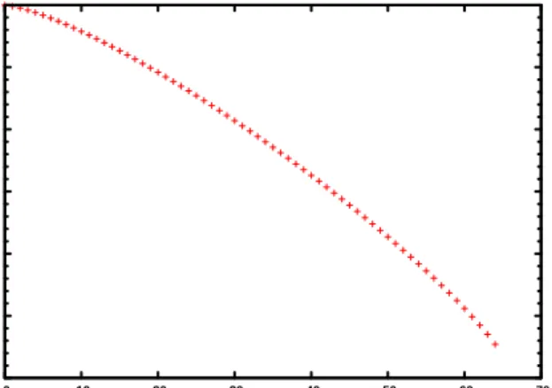
Figure 9(a) shows the probability of entering the crit-ical section for various values of max. Since the entry section contains waiting loops, the number of memory accesses of Pi before entering its critical section is un-bounded (and hence, also the costmax). However, the probability that a process waits indefinitely before en-tering its critical section tends to zero in long-term runs
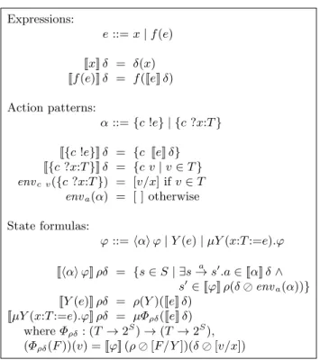


![Fig. 10: Execution time and memory consumption of CADP and PRISM for checking the six probabilistic properties in [18] on the BRP model for five retries and a packet size k between 16 and 256 data chunks.](https://thumb-us.123doks.com/thumbv2/123dok_us/1984912.2794787/20.892.82.820.137.1068/execution-memory-consumption-prism-checking-probabilistic-properties-retries.webp)