Wind power forecasting using historical data and artificial neural networks modeling

(1)

1

WIND POWER FORECASTING USING HISTORICAL

DATA AND ARTIFICIAL NEURAL NETWORKS

MODELING

K.P. Moustris

1,*

, D. Zafirakis

2

, K.A. Kavvadias

2,

J.K. Kaldellis

2

1_{Lab of Fluid Mechanics, Mechanical Engineering Department, Piraeus University of Applied Sciences, Petrou}

Ralli & Thivon 250, GR-12244, Aegaleo, Greece

2_{Lab of Soft Energy Applications & Environmental Protection, Mechanical Engineering Department, Piraeus}

University of Applied Sciences, Petrou Ralli & Thivon 250, GR-12244, Aegaleo, Greece

*_{kmoustris@yahoo.gr}

Keywords: Wind Power, Forecasting, Artificial Neural Networks

Abstract

One of the main parameters affecting the reliability of the renewable energy sources (RES) system, compared to the local conventional power station, is the ability to forecast the RES availability for a few hours ahead. To this end, the main objective of this work is the prognosis of the mean, maximum and minimum hourly wind power (WP) 8hours ahead. For this purpose, Artificial Neural Networks (ANN) modeling is applied. For the appropriate training of the developed ANN models hourly meteorological data are used. These data have been recorded by a meteorological mast in Tilos Island, Greece.

For the evaluation of the developed ANN forecasting models proper statistical evaluation indices are used. According to the results, the coefficient of the determination ranges from 0.285 up to 0.768 (mean hourly WP), from 0.227 up to 0.798 (maximum hourly WP) and from 0.025 up to 0.398 (minimum hourly WP). Furthermore, the proposed forecasting methodology shows that is able to give sufficient and adequate prognosis of WP by a wind turbine in a specific location 8 hours ahead. This will be a useful tool for the operator of a RES system in order to achieve a better monitoring and a better management of the whole system.

1 Introduction

Acknowledging the intermittent character of wind energy production and the fact that State subsidy in the form of feed-in-tariffs for such power producers gradually diminishes, the need for sufficient forecasting of wind power production is more than necessary. The purpose of wind power production is twofold. On the one hand, new wind parks will have to produce revenues through participation in wholesale, spot power markets; on the other, emerging smart grids require advanced energy management, prerequisite of which is also the development of sophisticated forecasting techniques. Furthermore, energy storage systems are essential for minimizing waste RES energy and

maximizing RES penetration as well as for the impact of WP on electricity prices [1]. Based on that concept, the ongoing European funded project “Technology Innovation for the Local Scale Optimum Integration of Battery Energy Storage (TILOS)” aims to demonstrate large-scale RES penetration through an optimum integration of wind - photovoltaic power station and advanced battery storage at Tilos Island, Greece. TILOS is a multinational European demonstration and research project with 15 participating enterprises and institutes from 7 European countries coordinated by the Lab of Soft Energy Applications & Environmental Protection of Piraeus University of Applied Sciences. One of the main parameters affecting the reliability of the RES system, compared to the local conventional power station, is the ability to forecast the RES availability for a few hours ahead. For that purpose, a great number of researchers have been worked on the forecast of the wind speed and wind power around the world during the last decade and beyond.

Wang et al. [2] presented a detailed review of wind speed forecasting, including the application of wind energy, time horizons for wind speed prediction and wind speed forecasting methods. In their work, eight strategies for realizing multi-step wind speed forecasting with machine-learning methods have been presented and 48 different hybrid models based on these eight strategies have been compared.

Shao and Deng [3] proposed a novel strategy in order to forecast the short-term WP using model structure selection in combined with data fusion technique. They presented a short-term wind power forecasting method using model structure selection technique in combined with four representative fusions of dimensionality reduction methods to optimize the model structure, promote the computational efficiency and improve the forecasting accuracy. In their work, experimental evaluation based on the real data from the wind farm in Jiangsu province is given to verify the effectiveness of the proposed method by comparing the traditional techniques.

Wang et al. [4] proposed a wind speed forecasting method based on improved empirical mode decomposition (EMD) and GA-BP artificial neural

(2)

2 network. They applied their methodology in a case study of a wind farm in Inner Mongolia, China. Results showed that the proposed hybrid method is much more accurate than the traditional GA-BP forecasting approach and GA-BP with EMD and wavelet neural network method.

Doucoure et al. [5] developed a prediction method for RES in order to achieve an intelligent management of a microgrid system and to promote the utilization of renewable energy in grid connected and isolated power systems. The proposed method was based on the multi-resolution analysis of the time-series by means of Wavelet decomposition and ANN. The analysis of predictability of each component of the input data using the Hurst coefficient was also proposed. In this context, using the information of predictability, it was possible to eliminate some components, having low predictability potential, without a negative effect on the accuracy of the prediction and reducing the computational complexity of the algorithm. In the evaluated case, it was possible to reduce the resources needed to implement the algorithm of about 29% by eliminating the two (of seven) components with lower Hurst coefficient. This complexity reduction has not impacted the performance of the prediction algorithm. Noorollahi et al. [6] in their paper presented an investigation of the management of wind intermittence in two parts, the prediction of wind speed in both temporal and spatial dimensions, using ANN modeling techniques. In the first part of their work the temporal dimension of wind speed at one-hour time interval, as a short-term wind speed prediction, in three wind observation stations (WOSs) in Iran was predicted. In the next part, estimation of wind speed data in a WOS using data from some other nearby WOSs was carried out. Due to the limitation of data collection, two groups of WOSs were selected for this target. The average value of the wind speed histogram error obtained from the best model in both groups is about 2.6% which is certainly promising.

Men et al. [7] used an ensemble of mixture density neural networks for short-term wind speed and power forecasting. Predicted wind speeds obtained from a numerical weather prediction model were used as the input data for the mixture density network, whose outputs are the mixture density parameters (used to represent the probability density function of the uncertain output or target variable). All mixture density ANN models in an ensemble were assumed to have a three-layer architecture, with each architecture having different numbers of nodes in the hidden layer. An application of the proposed approach to a data set of the measured wind speed and power from an operational wind turbine in a wind farm in Taiwan was used to evaluate the methodology. The results of this application demonstrate that the proposed methodology works well for the multi-step ahead wind speed and power forecasting.

In this context, the main objective of this work is the prognosis of the mean, maximum and minimum hourly wind power (WP) 8hours ahead at a specific location and a specific height in Tilos Island, Greece where a wind turbine of 800kW is going to be installed. For this purpose, (ANN) modeling is applied.

2 Methodology

2.1 Artificial Neural Networks Topology

For the forecasting of the mean hourly, the absolute maximum and minimum WP eight hours in advance artificial neural networks modeling was applied. ANN are based on the structure and function of the human brain. Neurons are basic components of the human brain. They are essential nerve cells which create a dense network. The first ANN models were introduced during the decades of 1940 and 1950 with the basic artificial neuron model of McCulloch and Pitts [8], along with the first ANNs training algorithm of Rosenblatt [9]. In the following decades the use of the ANNs showed significant decline, due to high computing power requirements, which were not available from the computers of that era. The recession was followed by regeneration of ANNs with the introduction of the Hopfield’s model [10-11]. These are known as Multi-Layer Perceptron (MLP) ANN, which along with the training algorithm of back-propagation, proposed by Werbos [12] attract the interest of the scientific community again.

Fig.1 Typical artificial neural network architecture [13] Figure 1 shows the architecture of a typical MLP artificial neural network as well as the training algorithm of back-propagation [13]. The first layer is the input layer with one or more neurons, depending on the number of necessary input data for the proper training of ANN. One or more hidden layers follow with a number of artificial neurons that are necessary for the processing of the input signals. Each neuron of the hidden layer communicates with all the neurons of the next hidden layer, if any, having in each connection a typical weight factor (Fig. 1). Finally, the signal reaches the output layer, where the output value from the ANN compares with the target value and the error is estimated. Thus, the values of the weight factors are

(3)

3 appropriately improved and the training cycle is estimated.

2.2. Data Management and ANN development In the present work, different ANN prognostic models were developed in order to forecast the mean, maximum and minimum hourly WP eight (8) consecutive hours in advance. For this purpose, appropriate meteorological data collected and analyzed to create the proper data base. More concretely, one minute intervals data of wind speed, wind direction and air pressure were collected from a meteorological mast (30m above ground level). The specific meteorological mast is located at the northernmost point of Tilos Island, Greece which is a few meters beyond the coast and about 10m above the sea level. The recorded data base is covering the time period from 17/03/2015 up to 29/02/2016 (almost a year).

Initially, the mean hourly, the absolute maximum and the absolute minimum wind speed during any hour of the examined period were calculated as well as the prevailing hourly wind direction and the mean hourly air pressure.

For the appropriate ANN training the whole data set was divided into two different subsets. These two subsets consider both wind speed and WP production obtained with the employment of an E-53 Enercon wind turbine power curve. The first subset contains all data from 17/03/2015 up to 17/02/2016 and was used as the training data set. The second subset contains data from 18/02/2016 up to 29/02/2016 (12 days). The second subset was totally unknown to the trained ANN forecasting model and was used for the validation of the forecasting ability of the developed ANN model. Three different MLP-ANN models were developed. The first (ANN1) forecasts the mean hourly WP (kW) for the next 8 consecutive hours. The second (ANN2) predicts the absolute maximum WP (kW) during each one of the next 8 consecutive hours and finally the third (ANN3) model forecasts the absolute minimum WP (kW) during each one of the next 8 consecutive hours. Table I presents the input data which have been used during the training phase of the developed ANN forecasting models as well as the output data (targets) in each case.

Table 1 Input and out put data of the developed ANN

Input Data (Input Layer) Output Data (Output Layer)

The minimum wind speed of the 8 previous hours The maximum wind speed of the 8 previous hours

The mean wind speed of the 8 previous hours The mean atmospheric pressure of the 8 previous hours

The minimum WP (kW) of the 8 previous hours The maximum WP (kW) of the 8 previous hours The mean WP (kW) of the 8 previous hours

ANN1 The mean hourly WP (kW) for the next 8 consecutive hours

(8 values)

ANN2 The absolute maximum WP (kW) during each hour of the next 8 consecutive hours

(8 values)

ANN3 The absolute minimum WP (kW) during each hour of the next 8 consecutive hours

(8 values) At this point is worthily to be mentioned that the three developed ANN prognostic models produce a dynamic forecast of WP for the next 8 consecutive hours. This means that every single hour of the day, the developed forecasting models are able to forecast the absolute minimum, the absolute maximum and the mean WP for each one of the next 8 consecutive hours of the day and so on. As a result of this procedure is that during the 24 hours of a day, the developed ANN models gives 24 forecasts and in each forecast predicts the next 8 consecutive values of WP (each model separately). 2.3. Statistical Evaluation Indices

For the evaluation of the forecasting ability of the developed ANN model, appropriate evaluation statistical indices were used. More specifically, the mean bias error (MBE), the root mean square error (RMSE), the coefficient of determination (R2) and the index of agreement (IA) were calculated in each case respectively. The MBE represents the degree of correspondence between the mean forecast and the mean observation. The MBE is used in order to describe how much the model underestimates or overestimates

the observed data. Positive or negative values indicate over estimated or under estimated prediction respectively [14].

The RMSE is a commonly used measure of the differences between the predicted values by a predictable model and the real-observed values. The RMSE is used as a single measure that indicates the ability of the model prediction and has the same units with the predicted value. The smaller the numerical value of RMSE is the closer to the real values are the predicted values by the model [14].

The coefficient of determination (R2_{) indicates how}

much of the observed variability is accounted by the estimated model [15]. The coefficient of determination is a number between 0 and +1 and measures the degree of association between two variables. The coefficient of determination is calculated according to the equation [16].

Finally, the IA is a dimensionless measure that is limited to the range of 0-1. If IA=0, that means no agreement between prediction and observation and if

(4)

4 IA=1, that means perfect agreement between prediction and observation. In other words, if IA=0 then the forecasted values present a great difference-distance in relation to the corresponding observed values and if IA=1 then all of the forecasted values are strictly equal to the corresponding observed values (i.e. predicted value=observed value for every forecasted value for each one of the forecasted values-cases) [17].

3 Results

3.1 WP statistical treatment

Initially, a statistical treatment of the hourly WP recorded values during the measuring period in Tilos Island, Greece took place. In Figure 2, the wind rose diagram representing the prevailing wind direction and the corresponding percentage of the observed WP.

Fig. 2 Wind rose diagram with the prevailing wind speed and the corresponding WP (kW). Tilos Island, Greece. Period 17/03/2015 up to 29/02/2016

According to Fig. 2 it is obvious that during the examined period the prevailing wind direction is the North-west. Also, when North-west winds prevailing a percentage of about 50% of the produced WP is less than 200kW and the rest is ranging between 200kW and 800kW.

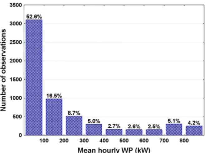
Figure 3 shows the WP frequency distribution during the examined period at the specific location in Tilos Island, Greece and for the specific wind turbine E-53 Enercon. As we can see, a percentage of about 52.6% presents WP less than 100kW. This means that during the half hours of the day the WP is less than 100kW indicating a low wind profile for the specific location. Only a rate of 17.1% shows WP production greater than or equal to 400kW.

Fig.3 Frequency distribution of the mean hourly WP Figure 4 depicts at the Box & Whiskers diagram of the absolute minimum, the absolute maximum and the average hourly WP.

Fig. 4 Box & Whiskers of absolute minimum, absolute maximum and average hourly WP

In Figure 4 it is obvious that during an hour of the day in the specific location in Tilos Island the absolute minimum WP is around 50kW. Also, the absolute maximum WP is close to 400 kW and finally the average WP is very close to 200kW.

3.2 ANN evaluation

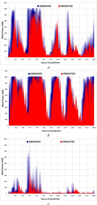
As mentioned above, the second data subset is composed with data from 18/02/2016 up to 29/02/2016 (12 days), is totally unknown to the trained ANN and is used for the validation of the trained ANN in each case. Figure 5 depicts the 8 hours ahead hourly moving prognosis of the mean hourly WP (a), the maximum hourly WP (b) and the minimum hourly WP (c) during the validation period from 18/02/2015 up to 29/02/2015 in Tilos Island, Greece. For the evaluation of the forecasting ability of the developed ANN models the aforementioned appropriate evaluation statistical indices were calculated. Table 2 presents the values of the evaluation statistical indices in each case (ANN1, ANN2 and ANN3) and for each one of the 8 consecutive forecasted hours respectively.

(5)

5 a

b

c

Fig. 5 Eight (8) hours in advance hourly moving prognosis of the mean hourly WP (a), the absolute maximum WP (b) and the absolute minimum WP (c) during the validation period from 18/02/2015 up to 29/02/2015 in Tilos Island, Greece

According to Figure 5 and Tables 2, 3 and 4 it seems that in general terms the forecasting ability of the three proposed ANN models is very good in an acceptable level of confidence. For such applications, it is crucial to the manager-operator of the system the previous knowledge of the mean, maximum and minimum hourly WP 8 hours in advance. The MBE in all forecasted hours for the three developed ANN models is negative. This indicates that in all cases the WP is underestimated. The IA is ranging from 0.931 to 0.696 (ANN1) and 0.943 to 0.674 (ANN2). This means that in case of mean hourly WP (ANN1) and absolute maximum hourly WP (ANN2) the predicted values are very close to the observed WP values.

In case of absolute minimum hourly WP the IA is ranging between 0.746 and 0.320. This shows a good agreement for such a stochastic variable magnitude as is the absolute minimum hourly WP from a wind turbine in a specific location, 8 hours in advance (e.g. the WP is equal to 0 for wind speeds lower than 5 m/s). The same conclusions are resulting taking into consideration the RMSE and R2_.

Table 2 Statistical evaluation indices for ANN1 AVEWP

HOURS

AHEAD MBE (kW) RMSE (kW) IA R2 1 -26.4 132.2 0.931 0.768 2 -34.9 170.9 0.875 0.616 3 -49.7 194.4 0.822 0.511 4 -48.0 210.0 0.797 0.436 5 -52.7 218.2 0.780 0.397 6 -64.0 223.3 0.751 0.370 7 -74.4 236.7 0.716 0.314 8 -78.5 243.6 0.696 0.285

Table 3 Statistical evaluation indices for ANN2 MAXWP HOURS

Table 4 Statistical evaluation indices for ANN3 AVEWP

HOURS

4 Conclusion

The main objective of the present work is the development of a prognostic tool in order to forecasts eight (8) hours ahead the absolute maximum, minimum as well as the mean hourly wind power which is produced by an E-53 Enercon wind turbine at a specific location in Tilos Island, Greece using real-recorded wind speed data and the corresponding wind turbine power curve.

(6)

6 Concluding, the proposed forecasting methodology shows that is able to give sufficient and adequate prognosis of wind prediction by a wind turbine in a specific location 8 hours in advance. This will be a useful tool for the operator of a RES system in order to achieve a better monitoring and a better management of the whole system.

5 Acknowledgements

This work took place and was funded under the project TILOS (Horizon 2020 Low Carbon Energy Local / small-scale storage LCE-08-2014).

This project has received funding from the European Union's Horizon 2020 research and innovation programme under Grant Agreement No 646529.

6 References

[1] Martinez-Anido, C.B., Brinkman, G., Bri-Mathias Hodge, B-M.: ‘The impact of wind power on electricity prices’, Renewable Energy, 2016, 94, pp. 474–487 [2] Wang, J., Song, Y., Liu, F.,, Hou, R.: ‘Analysis and application of forecasting models in wind power integration: A review of multi-step-ahead wind speed forecasting models’, Renewable and Sustainable Energy Reviews, 2016, 60, pp. 960–981

[3] Shao, H., Deng, X.: ‘Short-term wind power forecasting using model structure selection and data fusion techniques’, Electrical Power and Energy Systems, 2016, 83, pp. 79–86

[4] Wang, S., Zhang, N., Wu, L., Wang, Y.: ‘Wind speed forecasting based on the hybrid ensemble empirical mode decomposition and GA-BP neural network method’, Renewable Energy, 2016, 94, pp. 629-636

[5] Doucoure, B., Agbossou, K., Cardenas, A.: ‘Time series prediction using artificial wavelet neural network and multi-resolution analysis: Application to wind speed data’, Renewable Energy, 2016, 92, pp. 202-211 [6] Noorollah, Y., Jokar, M.A., Kalhor, A.: ‘Using artificial neural networks for temporal and spatial wind speed forecasting in Iran’, Energy Conversion and Management, 2016, 115, pp. 17–25

[7] Men, Z., Yee, E., Lien, F.-S., Wen, D., Chen, Y.: ‘Short-term wind speed and power forecasting using an ensemble of mixture density neural networks’, Renewable Energy, 2016, 87, pp. 203-211

[8] McCulloh, W.S and Pitts, W.: ‘A logical calculus of ideas immanent in Nervous activity’, B. Math. Biophys., 1943, 5, pp.115-133

[9] Rosenblatt, F.: ‘The Perceptron: A Probabilistic model for information storage and organization in the brain. Cornell Aeronautical Laboratory. Psychol. Rev., 1958, 65, 6, pp. 386-408

[10] Hopfield, J.J.: ‘Neural networks and physical systems with emergent collective computational abilities’, Proceedings of the National Academy of Sciences of the USA, 1982, 9, pp. 2554-2558

[11] Hopfield, J.J.: ‘Learning algorithms and probability distributions in feed-forward and feed-back networks’, Proceedings of the National Academy of Sciences of the USA, 1987, 84, pp. 8429-8433

[12] Werbos, P.: ‘Generalization of Backpropagation with application to a recurrent gas market model’ Neural Networks, 1988, 1, pp. 339-356

[13] Caudill, M., Butler, C.: ‘Understanding neural networks’, Cambridge, MA:MIT Press, ISBN 02625309996, 1992.

[14] Moustris, K.P., Ziomas, I.C., Paliatsos, A.G.: ‘3-Day-Ahead Forecasting of Regional Pollution Index for the Pollutants NO2, CO, SO2, and O3 Using Artificial Neural Networks in Athens, Greece’, Water Air Soil Poll., 2010, 200, pp. 29–43

[15] Kolehmainen, M., Martikainen, H., Ruuskanen, J.: ‘Neural networks and periodic components used in air quality forecasting’, Atmos. Environ., 2001, 35, pp. 815-825

[16] Comrie, A.C.: ‘Comparing neural networks and regression models for ozone forecasting’, J. Air Waste Manag. Assoc., 1997, 47, pp. 653-663

[17] Willmott, C.J., Ackleson, S.G., Davis, R.E., Feddema, J.J., Klink, K.M., Legates, D.R., O’Donnell, J., Rowe, C.: ‘Statistics for the evaluation and comparison of models’, J. Geophys. Res., 1985, 90, pp. 8995-9005