Time series ordinal classification via shapelets
David Guijo-Rubio
Dept. of Computer Scienceand Numerical Analysis University of C´ordoba
C´ordoba, Spain. [email protected] 0000-0002-8035-4057
Pedro A. Guti´errez
Dept. of Computer Scienceand Numerical Analysis University of C´ordoba
C´ordoba, Spain. [email protected] 0000-0002-2657-776X
Anthony Bagnall
School of Computing SciencesUniversity of East Anglia Norwich Research Park Norwich, United Kingdom.
[email protected] 0000-0003-2360-8994
C´esar Herv´as-Mart´ınez
Dept. of Computer Scienceand Numerical Analysis University of C´ordoba
C´ordoba, Spain. [email protected] 0000-0003-4564-1816
Abstract—Nominal time series classification has been widely developed over the last years. However, to the best of our knowledge, ordinal classification of time series is an unexplored field, and this paper proposes a first approach in the context of the shapelet transform (ST). For those time series dataset where there is a natural order between the labels and the number of classes is higher than 2, nominal classifiers are not capable of achieving the best results, because the models impose the same cost of misclassification to all the errors, regardless the difference between the predicted and the ground-truth. In this sense, we consider four different evaluation metrics to do so, three of them of an ordinal nature. The first one is the widely known Information Gain (IG), proved to be very competitive for ST methods, whereas the remaining three measures try to boost the order information by refining the quality measure. These three measures are a reformulation of the Fisher score, the Spearman’s correlation coefficient (ρ), and finally, the Pearson’s correlation coefficient (R2). An empirical evaluation is carried out, considering 7 ordinal datasets from the UEA & UCR time series classification repository, 4 classifiers (2 of them of nominal nature, whereas the other2are of ordinal nature) and 2 performance measures (correct classification rate, CCR, and average mean absolute error, AM AE). The results show that, for both performance metrics, the ST quality metric based on
R2 is able to obtain the best results, specially for AM AE, for which the differences are statistically significant in favour ofR2.
Index Terms—Time Series, Ordinal Classification, Ordinal regression, Shapelet Quality Measures
I. INTRODUCTION
Time series are a widely used sort of temporal data in which objects are collected over time. In the last years, time series have been a hot topic in machine learning and data mining, and can be found in a vast number of fields such as: fog prediction [1], stock indices [2] or forged-alcohol detection [3]. Time series classification is a task in which a label is given to a set of chronologically ordered points. We focus on a specific case, those problems in which there are three or more possible categories and they follow an order relationship.
This kind of classification is known as ordinal classifica-tion or ordinal regression, being a field of machine learning tackling problems in which the target variables are discrete and present a natural order between their labels [4]. An
example is the prediction of the stage of a disease state, in which a patient could be labelled asnone,mild,moderate, severeorextreme. Obviously, misclassifying amildpatient as severe, should be far more penalised than misclassifying that patient as none or moderate. This problem can be tackled in several ways: 1) as a nominal classification problem, which ignores the natural order between the labels, 2) as a regression problem, which implies assigning each label a numerical value (which requires assuming a distance between values that can hinder the performance of the regressor), or 3) as an ordinal classification problem, which is the approach we consider. This special kind of classification can be found in several fields, such as meteorological prediction [5], medical research [6], [7] and wave height prediction [8]. The datasets used in these projects include an ordered target variable, and thus, specialised ordinal classifiers are able to achieve higher performances than nominal classifiers or regressors, by constructing more accurate models.
Traditionally, nominal time series have been classified using a similarity measure in conjunction with a standard classifier, such as k-Nearest Neighbours [9]. This similarity can be assessed from several points of view: by considering time, change or shape. We focus on shape based similarity, in which time series are compared by using phase independent sub-sequences generally much shorter than the original time series. These sub-sequences, known as shapelets,were first proposed as a time series primitive by Ye and Keogh [10]. The original proposal embedded the shapelet extraction into a decision tree that used Information Gain (IG) to assess the candidates. Moreover, this time series primitive has been used in some other ways in the literature: Hills et al. [11] proposed the Shapelet Transformation (ST), in which the k best shapelets are used to convert the original time series dataset into a new transformed dataset. In this new representation, the attributes are the distances between the shapelets and the time series being evaluated. The reason for this is that the transformation allows the application of any classifiers and avoids the sequen-tial search for shapelets at each node of the tree. Grabocka et al.[12] proposed a new perspective in which shapelets are learned. This method enables the learning of shapelets without the need of searching for a vast number of candidates.
In this paper, the perspective of Hills et al. [11] has been considered. We study two different elements in which the ordinal information can be included in the ST time series classification process: the quality measure and the final clas-sifier. One key point is the selection of the best k shapelets, performed by assessing the shapelet quality. Therefore, we evaluate different ordinal shapelet quality measures and com-pare them against the state-of-the-art IG metric, which has proved to be very competitive for nominal classification [11]. To further exploit the ordinal nature of the data, after the ST, we consider specifically designed classifiers for ordinal classification. Our principal hypothesis is that the ST using IG would not be able to achieve the best results just by the application of ordinal classifiers. However, when these ordinal classifiers are applied to the transformed data performed by “ordinal” shapelets (those shapelets assessed by a quality measure favouring the ordinal information), the results should take advantage of both mechanisms. Specifically, for this work, the well-known Proportional Odds Model (POM) and Support Vector for Ordinal Regression with IMplicit constrains (SVORIM) are compared against two nominal classifiers also based on Support Vector Classifiers (SVC1V1 and SVC1VA). The main objectives of this paper are: 1) To firstly draw attention to the problem of ordinal classification of time series, selecting different ordinal datasets from the popular UEA & UCR Time Series Classification Repository1. 2) To adapt one
of the most popular method in the literature, the ST, to the ordinal classification field, by introducing new ordinal quality metrics that could take advantage of the ordinal nature of the dataset (i.e. to make preferable those shapelets maximising the amount of ordinal information) and by replacing nominal classifiers by ordinal ones.
The remainder of this paper is organized as follows: In Section II, the concepts of time series and shapelets are briefly described, along with the details of the different shapelet quality measures proposed (Section II-A). Ordinal classifiers and their performance evaluation metrics are detailed in Sec-tion II-B. The experimental results and discussion are exposed in Section III, including the datasets (Section III-A) and the experimental settings used (Section III-B), as well as, the results and the statistical test (Section III-C). Finally, Section IV concludes the paper with some final remarks.
II. BACKGROUND
Time series is a special kind of data in which values are collected chronologically. More formally, a time series classification dataset,T={T1,T2, . . . ,TN}, is composed of
N time seriesTi ={t1, t2, . . . , tn}, i∈ {1, . . . , N}, each of
them including in turnnreal values and a class valueCi∈Y.
In this paper, all the datasets considered only include equal-length time series (i.e. n is constant). Furthermore, given the nature of the datasets used, they are considered as ordinal datasets, this is, a natural order exists among the labels, i.e. Y ={C1,C2, . . . ,CQ}, where Q is the number of categories
1http://www.timeseriesclassification.com/
and {C1,C2, . . . ,CQ} are the ordinal labels, satisfying the
constraintC1≺C2≺. . .≺CQ.
A. Time Series Shapelets
Time series nominal classification is a well-known field, in which a huge variety of approaches to classify time series have been proposed [13]. Currently, the best approach to standard classification is HIVE-COTE [14], a meta-ensemble including five different modules with several algorithms in each one. Some of these modules rely on the idea of transforming the original dataset prior to classification. As a first approach, in this paper, we decided to focus on the Shapelet Transform (ST), in which the transformed attributes represent the shape-similarity between the original time series and the shapelets, phase independent subsequences of the time series forming a new primitive for time series classification. It was firstly proposed by Ye and Keogh [10], [15], yet improved versions and new perspectives have been presented in the literature [11], [12], [16], [17], among others.
A shapelets={s1, s2, . . . , sl} is a subsequence of a time
series Ti, wherel ≤n. The shapelet extraction procedure is
divided into three main separate steps [11] (see Algorithm 1): 1) candidate generation, i.e. generation of a subsequence satisfying the previous length constraint, 2) measuring sim-ilarity between the candidate and the time series, and 3) measuring quality of the candidate. Once the bestkshapelets are extracted, ST creates a new representation of the original dataset, where each attribute represents a shapelet, and its values are the distances between the shapelet and the original time series. It is worthy of mention that we have used the most recent version of ST [17]: the Euclidean distance is used to measure the distance between the shapelets and the time series (this distance is computed as the minimum of the distances between the shapelet and all possible subsequences of the time series with the same length of the shapelet). Furthermore, this method balances the number of shapelets extracted per class, and evaluates each shapelet using the binary Information Gain [18] (IG).
This paper proposes to consider different shapelet quality measures in order to incorporate the ordinal nature of the labels into the ST extraction. As a baseline, we will compare the results against the use of the most popular metric, the IG, which measures how well the shapelet class is discriminated from the rest according to the set of distances between the shapelet and the time series. First, we obtain the set of distances,ds,Ti, i∈ {1, . . . , N}, from the evaluated shapelet
s to all the time series Ti. Once this set is sorted, all the
possible split points (being the split point, the average point between two consecutive distances) are evaluated, storing the best IG split point. The IG is defined as:
IG(s) = max
sp∈ds,Ti
IG(sp), (1)
Algorithm 1 Main steps of the Shapelet Transform (ST).
Input: Time series dataset 1: S← ∅// Shapelet set 2: forEach time seriesTi do
3: STi ← ∅
4: bestQuality←0 5: forl←mintomaxdo
6: Pl←Generate candidates(Ti,l)
7: forCandidatesinPl do
8: ds,Ti ←Calculate distances(s,Ti)
9: quality←Evaluate candidate (s,ds,Ti)
10: ifquality > bestQuality then
11: STi ←s 12: bestQuality←quality 13: end if 14: end for 15: end for 16: S←STi 17: SortS by quality
18: Remove similar shapelets inS 19: end for
20: return Best shapelet setS
(sp), and it is expressed as:
IG(sp) =H(ds,Ti)− |s− p| |ds,Ti| H(|s− p|) + |s+ p| |ds,Ti| H(|s+ p|) , (2) where s−
p are the elements of the sorted distance set located at the left of the split point,sp, whereass+p are the remaining elements. Moreover, |ds,Ti| andH(ds,Ti)are the cardinality
and the entropy of the setds,Ti, respectively, being the entropy
defined as:
H(ds,Ti) =−
X
c∈Y
pc log pc, (3)
wherepc is the a priori probability of classc.
Note that this version of ST using IG takes advantage of early abandon of the shapelet evaluated, when the most optimistic IG obtained is worse than that obtained by the best shapelet found so far. This takes place after obtaining every value ofds,Ti, where the most optimistic situation is supposed
for the rest of time series, i.e. the one giving the highest value for IG. Hence, if this is worse than the best shapelet found so far, the distances from shapeletsto the remaining time series
Ti do not need to be calculated.
As the main objective of the paper is the ordinal classifica-tion of time series, three different shapelet quality measures are proposed in order to obtain shapelets minimising the most severe errors in the ordinal scale. The first of these measures is based on the Fisher score [19], commonly used for feature selection. A reformulation of this score has been made in order to adapt it to ordinal classification, known as Ordinal Fisher (OF) [20] score. This reformulation is based on the inclusion of higher costs for distant classes, i.e. the cost depends on the distance between the shapelet class and the class of the
time series being compared. The reason behind this proposal is that distant classes should be associated higher distances. The reformulation is defined as follows:
OF(s) = PQ k=1 PQ j=1|k−j|(¯xk−¯xj) 2 (Q−1)PQ k=1(Sk)2 , (4)
wherex¯k andSk are the mean and standard deviation of the
distances according to the shapelet s when considering time series of the classCk, and|k−j|is the number of categories
betweenCk andCj, penalising farther classes.
A different approach to measure the quality of the shapelets, maximising the ordinal information, is a modified version of the Pearson’s correlation coefficient (R2), that calculates the correlation between the distances obtained from the shapelet, ds,Ti, and the difference of their class indices. First of all, we
define the difference between the class of the shapelet sand the time series ias:
cs,Ti =|O(Cj)− O(Ci)|, (5)
where Cj is the class of shapelet s, and O(Cq) = q, q ∈
{1, . . . , Q}, i.e. O(Cq) is the position of the category in the
ordinal scale.
From these values, the Pearson’s correlation coefficient (R2) can be expressed as:
R2(s) = N X i=1 S(ds,Ti, cs,Ti) Sds,TiScs,Ti , (6)
whereds,Tiis the distance between the shapeletsand thei-th
time series,Ti, andS(ds,Ti, cs,Ti)is the covariance between
ds,Ti andcs,Ti.
Finally, the last shapelet quality measure proposed is the Spearman’s correlation coefficient (ρ), which calculates the correlation between two variables that could be either categor-ical or continuous. As in the previous case, a reformulation of this score is performed so as to introduce ordinal information. The equation is the following:
ρ(s) = 1−6 PN
i=1D(s,Ti)2
N(N2−1) , (7)
whereD(s, Ti)2is the squared difference between ranks, being
expressed as:
D(s,Ti)2= (R(ds,Ti)− R(cs,Ti))
2
, (8)
whereR(x)is the rank ofxin the set of all values obtained. When comparing the different metrics analysed in this subsection, it should be highlighted that OF is the only metric which does not take into account the category of the shapelet being evaluated (s), only evaluating the separability obtained in accordance to the ordinal scale.
In order to ease the readability of the paper, from now on, the ST version that assess the shapelet quality using the R2 measure will be simply referred to as R2 (and the same will be done for the rest of quality metrics).
B. Ordinal classification
Once the datasets are constructed according to the ST, classifiers are learned on this new data. We include both nominal and ordinal classifiers to demonstrate that a better performance can be achieved taking advantage of the nature order between the labels [21]2:
• The Proportional Odds Model (POM) [22] is a
general-ized linear model that is based on cumulative probabilities according to the ordered labels. The cumulative probabili-ties are obtained using thelogitas link function (although other functions can be considered), considering the same linear one-dimensional projection but different ordered thresholds. In this sense, the model is a generalisation of binary logistic regression.
• The Support Vector for Ordinal Regression (SVOR) methodology is the adaptation of support vector machines to ordinal regression [23]. Specifically, the SVOR version considering IMplicit constrains (SVORIM) [24] consists in computing the discriminant parallel hyperplanes for the data, assuring the constraints of the thresholds implicitly, by considering patterns from all the categories to compute the error of the hyperplane of one category.
• The method Support Vector Classifier (SVC) [25] using
the one versus one formulation (SVC1V1) and the one vs all paradigm (SVC1VA) are also considered. These methods have been widely used in the literature as very competitive for both binary and nominal multiclass problems. We include them to check whether ordinal classifiers are able to further exploit order information. Finally, given that we are considering ordinal classification problems, we can not only rely on the accuracy as evaluation metric, because it simply ignore order information (all the mis-classification errors are equally penalised). There are several metrics to measure the performance of ordinal classifiers [26]. In this paper, we have focus on:
• Correct Classification Rate (CCR) or accuracy, which is
the global performance of the classifier. It is measured as follows: CCR= 100 N N X j=1 I(Cj,yˆj), (9)
where N is the total number of examples, I(·) is the zero-one loss function, and Cj and yˆj are the true and
the predicted label for the time seriesTj.
• Average Mean Absolute Error (AM AE) [27] measures
the ordinal classification errors made for every class. It is obtained as: AM AE= 1 Q Q X q=1 M AEq, (10)
2These classifiers are available in the repository https://github.com/ayrna/
orca.
where M AEq is the Mean Absolute Error of class q,
defined as: M AEq= 1 Nq Nq X j=1 |O(Cj)− O(ˆyj)|, (11)
whereNq is the number of patterns belonging to classq.
CCR is a performance metric that varies between 0 and 100 and should be maximised, whereas AM AE is an er-ror measure varying between 0 and Q−1 and should be minimised. Note that standard performance metrics, such as CCR, are not able to give different cost for different errors (i.e. the cost of misclassifying a pattern is the same regardless the predicted class),. Thus, when dealing with ordinal datasets, more attention should be given to ordinal performance metrics, such asAM AE.
III. EXPERIMENTAL RESULTS AND DISCUSSION This section includes a description of the ordinal time series datasets used and the experimental settings for the four different classifiers chosen for this experiment, as well as a discussion of the results obtained 3.
A. Ordinal time series considered
TABLE I shows the datasets used. Given that this is the first time that time series ordinal classification is studied, a subset of 7 time series datasets has been appropriately chosen from the original UCR data repository [28]. Most of the datasets selected come from the field of bone age prediction, presented in [29]. Specifically, those named “AgeGroup” include patterns (bones) labelled asinf ant,juniororteen, depending on the age group to which the bone belongs. For those named “TW”, patterns are labelled by a human expert using the Tanner-Whitehouse score (6 different stages). On the other hand, the EthanolLeveldataset is part of a project to detect forged spirits using non-intrusive methods [3]. In this case, the labels of the dataset are the most common ethanol content (35%,38%,40% and45%).
The imbalanced ratio (IR) is included in TABLE I in order to check if the distribution of the patterns of a dataset leads to rare classes (high IR value). In these datasets, focusing only in theCCRcan lead to trivial classifiers, whileAM AEis better suited, because, apart from considering order information, it averages the individual performance of each class. According to [30], the Imbalance Ratio (IR) is defined as:
IR= 1 Q Q X q=1 IRq, IRq= P j6=qNj Q·Nq , (12)
whereIRj is the IR for the classj, andNq is the number of
patterns belonging to class Cj.
3All the code used in this paper is available from the repositoryhttps://
TABLE I
CHARACTERISTICS OF THE DATASETS USED IN THE EXPERIMENTS.Q:
NUMBER OF CLASSES, #TR:NUMBER OF TRAIN ELEMENTS, #TE:
NUMBER OF TEST ELEMENTS, LEN:TIME SERIES LENGTH, %IR:
IMBALANCED RATIO.
Dataset Q #TR #TE LEN %IR
DistalPhalanxOutlineAgeGr 3 400 139 80 1.532 DistalPhalanxTW 6 400 139 80 1.577 EthanolLevel 4 504 500 1751 0.750 MiddlePhalanxOutlineAgeGr 3 400 154 80 0.881 MiddlePhalanxTW 6 399 154 80 1.276 ProximalPhalanxOutlineAgeGr 3 400 205 80 0.951 ProximalPhalanxTW 6 400 205 80 2.203 B. Experimental settings
The main shapelet transformation code as well as the IG shapelet quality measure have been obtained from thesktime
toolkit [31] 4.
The ST method, regardless of the shapelet quality measure, is run for a one hour shapelet search. The results achieved are on the standard train and test splits given in the time series classification repository. Furthermore, it must be said that the test sets are only used to assess the learned models (adjusted on the training data). The ST using Information Gain (IG) as quality measure is usually set an inferior limit of0.05 to avoid keeping lowest-quality shapelets (this is the default value considered in sktime toolkit). In order to obtain a similar behaviour for the ordinal shapelet quality measures, the worst 10% of shapelets are removed, according to the metric evaluated.
Regarding the four ordinal classifiers, they have been run once, since all of them are deterministic. Note that previous to the application of these models, the transformed datasets are standardized and, in order to cross-validate their sensitive hyper-parameters, a nested10-fold cross-validation procedure has been run on the training set withAM AEas the parameter selection criteria. Three of the ordinal classifiers are SVM-based (SVORIM, SVC1V1 and SVC1VA), hence, the range {10−3,10−2, . . . ,103} is used to adjust the cost parameter and the kernel width. On the other hand, POM does not have hyper-parameters to be optimized.
C. Results
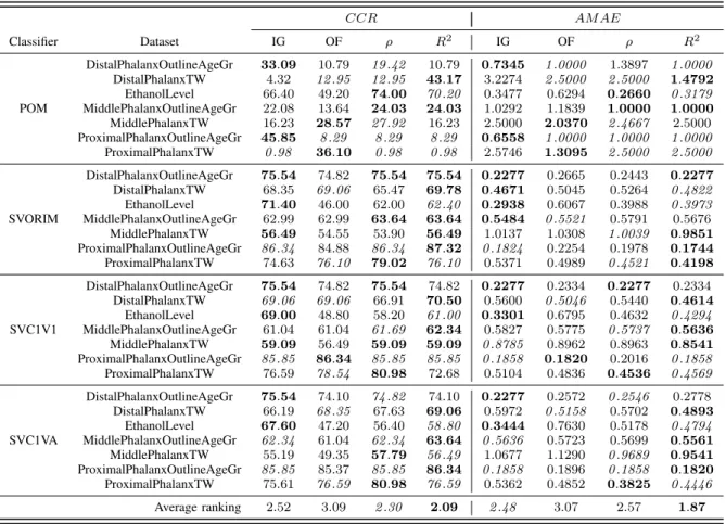
TABLE II presents the results obtained for the four shapelet quality measures and the different classifiers compared. More-over, we obtain the average rankings of each shapelet quality measure, considering all datasets and all classifiers. As shown in the TABLE II, the R2 measure generally leads to the best results in AM AE (which is the metric that better represents the ordinal classification task) andCCR(the one representing the global performance). The rest of the methods lead to worse results in AM AE, reflecting that the misclassification errors involve more categories of the ordinal scale. In accuracy
4Code is available in the website https://github.com/alan-turing-institute/
sktime.
(CCR), ST using IG,ρandR2 leads to more similar results (although the final average rank is still better forR2). In both metrics, OF method generally leads to worse results, which is probably due to the fact that the OF metric does not consider the class of the shapelet being evaluated.
Quantitative results show that, in terms ofCCR, IG is able to achieve the best or the second best results for16cases, OF in11cases,ρin21occasions, and, finally,R2,23times.R2 leads to aCCR rank of2.09, whereas the ST versions using the remaining shapelet quality measures,ρ, IG and OF, obtain a rank of2.30,2.52and3.09, respectively. On the other hand, in terms ofAM AE,R2 is also the one that achieves the best or the second best results more times, concretely, 24 times, whereas the other versions of ST are less accurate,15,15and 9 times forρ, IG and OF, respectively. These results lead to anAM AE ranks of1.87for R2 and2.48,2.57and3.07for IG,ρand OF, respectively.
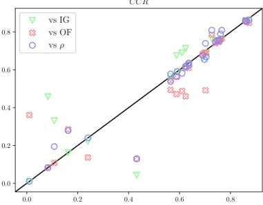
Furthermore, Fig. 1 and Fig. 2 show the results exposed in TABLE II graphically as scatter plots. R2 has been chosen as the reference method, given that is the one achieving the best rankings for both CCR and AM AE (2.09 and 1.87, respectively). In these scatter plots, points represent the comparison (in terms of CCR and AM AE) between the performance achieved by the ST usingR2 as shapelet quality measure against one of the alternative measure on a single dataset. Note that the x-axis of the scatter plot represents the performance obtained by the R2 method, whereas y-axis represents the performance achieved by the compared method, depending on its symbol and colour, shown in the legends. In this way, regarding Fig. 1 where theCCR is considered, points below the straight black line, represent those datasets for whichR2is able to obtain a higher performance, asCCR needs to be maximised. On the other hand, regarding Fig. 2, R2 wins are those points above the straight black line, since AM AE should be minimised. 0.0 0.2 0.4 0.6 0.8 0.0 0.2 0.4 0.6 0.8 CCR vs IG vs OF vsρ
Fig. 1. CCRresults comparingR2(x-axis) against the rest of the methods (y-axis).
TABLE II
CCRANDAM AERESULTS OBTAINED BY THE FOUR SHAPELET EXTRACTION METHODS COMPARED FOR THE SEVEN DATASETS AND THE FOUR
ORDINAL CLASSIFIERS. CCR AM AE Classifier Dataset IG OF ρ R2 IG OF ρ R2 POM DistalPhalanxOutlineAgeGr 33.09 10.79 19.42 10.79 0.7345 1.0000 1.3897 1.0000 DistalPhalanxTW 4.32 12.95 12.95 43.17 3.2274 2.5000 2.5000 1.4792 EthanolLevel 66.40 49.20 74.00 70.20 0.3477 0.6294 0.2660 0.3179 MiddlePhalanxOutlineAgeGr 22.08 13.64 24.03 24.03 1.0292 1.1839 1.0000 1.0000 MiddlePhalanxTW 16.23 28.57 27.92 16.23 2.5000 2.0370 2.4667 2.5000 ProximalPhalanxOutlineAgeGr 45.85 8.29 8.29 8.29 0.6558 1.0000 1.0000 1.0000 ProximalPhalanxTW 0.98 36.10 0.98 0.98 2.5746 1.3095 2.5000 2.5000 SVORIM DistalPhalanxOutlineAgeGr 75.54 74.82 75.54 75.54 0.2277 0.2665 0.2443 0.2277 DistalPhalanxTW 68.35 69.06 65.47 69.78 0.4671 0.5045 0.5264 0.4822 EthanolLevel 71.40 46.00 62.00 62.40 0.2938 0.6067 0.3988 0.3973 MiddlePhalanxOutlineAgeGr 62.99 62.99 63.64 63.64 0.5484 0.5521 0.5791 0.5676 MiddlePhalanxTW 56.49 54.55 53.90 56.49 1.0137 1.0308 1.0039 0.9851 ProximalPhalanxOutlineAgeGr 86.34 84.88 86.34 87.32 0.1824 0.2254 0.1978 0.1744 ProximalPhalanxTW 74.63 76.10 79.02 76.10 0.5371 0.4989 0.4521 0.4198 SVC1V1 DistalPhalanxOutlineAgeGr 75.54 74.82 75.54 74.82 0.2277 0.2334 0.2277 0.2334 DistalPhalanxTW 69.06 69.06 66.91 70.50 0.5600 0.5046 0.5440 0.4614 EthanolLevel 69.00 48.80 58.20 61.00 0.3301 0.6795 0.4632 0.4294 MiddlePhalanxOutlineAgeGr 61.04 61.04 61.69 62.34 0.5827 0.5775 0.5737 0.5636 MiddlePhalanxTW 59.09 56.49 59.09 59.09 0.8785 0.8962 0.8963 0.8541 ProximalPhalanxOutlineAgeGr 85.85 86.34 85.85 85.85 0.1858 0.1820 0.2016 0.1858 ProximalPhalanxTW 76.59 78.54 80.98 72.68 0.5104 0.4836 0.4536 0.4569 SVC1VA DistalPhalanxOutlineAgeGr 75.54 74.10 74.82 74.10 0.2277 0.2572 0.2546 0.2778 DistalPhalanxTW 66.19 68.35 67.63 69.06 0.5972 0.5158 0.5702 0.4893 EthanolLevel 67.60 47.20 56.40 58.80 0.3444 0.7630 0.5178 0.4794 MiddlePhalanxOutlineAgeGr 62.34 61.04 62.34 63.64 0.5636 0.5723 0.5699 0.5561 MiddlePhalanxTW 55.19 49.35 57.79 56.49 1.0677 1.1290 0.9689 0.9541 ProximalPhalanxOutlineAgeGr 85.85 85.37 85.85 86.34 0.1858 0.1896 0.1858 0.1820 ProximalPhalanxTW 75.61 76.59 80.98 76.59 0.5362 0.4852 0.3825 0.4446 Average ranking 2.52 3.09 2.30 2.09 2.48 3.07 2.57 1.87 0.0 0.5 1.0 1.5 2.0 2.5 3.0 0.0 0.5 1.0 1.5 2.0 2.5 3.0 AMAE vs IG vs OF vsρ
Fig. 2. AM AEresults comparingR2(x-axis) against the rest of the methods (y-axis).
Regarding the classifiers, the average CCR ranks of each classifier (considering all the datasets and all the ST methods) are 3.68, 1.95, 1.91 and 2.46, for POM, SVORIM, SVC1V1
and SVC1VA, respectively (i.e. SVC1V1 is slightly better than SVORIM, which is natural as CCR does not consider the ordering). However, when average AM AE ranks are considered, the values are 3.71 1.91 1.96 2.41, for POM, SVORIM, SVC1V1 and SVC1VA, respectively, which means that, in AM AE, SVORIM is slightly better. What is clear is that, from the classifiers compared, the POM is clearly the worst. Two main reasons can be found for this: POM is a linear method, and the implementation considered does not include a regularization term, which seems to be necessary, given the high number of shapelets extracted.
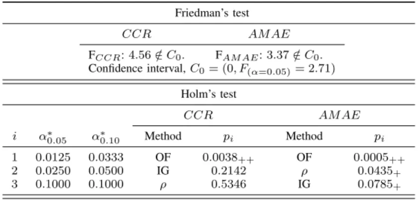
Fig. 1 and Fig. 2 show that the differences between the pro-posed methods are observable, specially for AM AE, highly affected by those cases where the predicted label is far, in the ordinal scale, from the ground truth. On the other hand, for CCR, the points are more dispersed due to this measure is pre-ferred for nominal classification. However, in order to check the existence of statistically significant differences in these results, we follow the procedure recommended by Demˇsar [32]. Specifically, after applying the non-parametric statistical Friedman’s test [33] to theCCR andAM AE rankings (see TABLE III), we reject the null-hypothesis stating that there are no differences in the results (for a significance level of α= 0.05). Once, these differences are assessed, we continue
the study by considering the post-hoc Holm’s test [34], which compares the different methods against a control method (in our case,R2method as it leads to the bestCCRandAM AE rankings). This test performs the comparisons sequentially in accordance to the ranking order, adjusting the significance level to compensate for multiple comparisons. As can be checked in TABLE III, the difference favouring theR2metric is statistically significant forAM AE when compared against the other three metrics (OF with significance level α= 0.05, and ρ and IG with significance level α = 0.10), while the CCR differences are only significant when it is compared against OF (significance level α= 0.05).
IV. CONCLUSIONS
This paper presents the first approach to ordinal classi-fication of time series, up to the authors’ knowledge. For this purpose, the Shapelet Transform (ST) is applied. Once the best k shapelets (assessed by a quality measure) are extracted, a transformation of the dataset is obtained, in which the attributes represent the shapelets, and the values of the attribute are the distances between the shapelet and the original time series. In this sense, three versions of the ST using different shapelet quality measures are proposed, in order to select those shapelets that maximise the ordinal information implicitly exposed in the datasets: Ordinal Fisher (OF), Pearson’s correlation coefficient (R2) and Spearman’s correlation coefficient (ρ). Finally, these proposals are then compared against the standard ST using the information gain (IG).
An experimental comparison of these 4 versions of ST is performed using 7 ordinal datasets (from the time series classification repository [35]) and 4 ordinal classifiers. The results are reported using theCCRandAM AEperformance metrics. The results achieved show that a ST combined with R2 is able to achieve the best results, specially in terms of AM AE, where the difference against the other approaches is statistically significant. In terms of accuracy (CCR), this approach obtained a better rank, meaning that the results are better than the obtained for the rest of the methods, yet they are not statistically significant, except when compared against OF. Given that standard accuracy does not take into account the ordinal scale, it is natural that the differences are lower.
As future work, three interesting avenues for research would be: 1) the consideration of an early abandon procedure for ordinal quality metrics to avoid unnecessary distance calculus in the shapelet extraction step; 2) the development of a distance metric, different from the euclidean, able to introduce different costs depending on the difference of the class of the shapelet and the class of the time series (in the ordinal scale); 3) and, finally, the adaptation of other modules of the HIVE-COTE meta-ensemble to ordinal classification.
ACKNOWLEDGEMENTS
This work has been subsidised by the by the TIN2017-85887-C2-1-P and the TIN2017-90567-REDT projects of the Spanish Ministry of Economy and Competitiveness
(MINECO) and FEDER funds (EU). David Guijo-Rubio’s research has been subsidised by the FPU Predoctoral Program (Spanish Ministry of Education and Science), grant reference FPU16/02128.
REFERENCES
[1] D. Guijo-Rubio, P. Guti´errez, C. Casanova-Mateo, J. Sanz-Justo, S. Salcedo-Sanz, and C. Herv´as-Mart´ınez, “Prediction of low-visibility events due to fog using ordinal classification,”Atmospheric Research, vol. 214, pp. 64–73, 2018.
[2] A. M. Dur´an-Rosal, M. de la Paz-Mar´ın, P. A. Guti´errez, and C. Herv´as-Mart´ınez, “Identifying market behaviours using european stock index time series by a hybrid segmentation algorithm,” Neural Processing Letters, vol. 46, no. 3, pp. 767–790, 2017.
[3] J. Large, E. K. Kemsley, N. Wellner, I. Goodall, and A. Bagnall, “Detect-ing forged alcohol non-invasively through vibrational spectroscopy and machine learning,” inPacific-Asia Conference on Knowledge Discovery and Data Mining. Springer, 2018, pp. 298–309.
[4] P. A. Guti´errez, M. P´erez-Ortiz, J. S´anchez-Monedero, F. Fernandez-Navarro, and C. Herv´as-Mart´ınez, “Ordinal regression methods: survey and experimental study,”IEEE Transactions on Knowledge and Data Engineering, vol. 28, no. 1, pp. 127–146, 2016.
[5] D. Guijo-Rubio, C. Casanova-Mateo, J. Sanz-Justo, P. Guti´errez, S. Cornejo-Bueno, C. Herv´as, and S. Salcedo-Sanz, “Ordinal regression algorithms for the analysis of convective situations over madrid-barajas airport,”Atmospheric Research, vol. 236, p. 104798, 2020.
[6] M. P´erez-Ortiz, M. Cruz-Ram´ırez, M. D. Ayll´on-Ter´an, N. Heaton, R. Ciria, and C. Herv´as-Mart´ınez, “An organ allocation system for liver transplantation based on ordinal regression,”Applied Soft Computing, vol. 14, pp. 88–98, 2014.
[7] M. P´erez-Ortiz, A. S´aez, J. S´anchez-Monedero, P. A. Guti´errez, and C. Herv´as-Mart´ınez, “Tackling the ordinal and imbalance nature of a melanoma image classification problem,” in 2016 International Joint Conference on Neural Networks (IJCNN). IEEE, 2016, pp. 2156–2163. [8] D. Guijo-Rubio, A. M. Dur´an-Rosal, A. M. G´omez-Orellana, P. A. Guti´errez, and C. Herv´as-Mart´ınez, “Distribution-based discretisation and ordinal classification applied to wave height prediction,” in Inter-national Conference on Intelligent Data Engineering and Automated Learning. Springer, 2018, pp. 171–179.
[9] H. Ding, G. Trajcevski, P. Scheuermann, X. Wang, and E. Keogh, “Querying and mining of time series data: Experimental comparison of representations and distance measures,” in Proc. 34th International Conference on Very Large Data Bases (VLDB), 2008.
[10] L. Ye and E. Keogh, “Time series shapelets: a new primitive for data mining,” inProceedings of the 15th ACM SIGKDD international conference on Knowledge discovery and data mining. ACM, 2009, pp. 947–956.
[11] J. Hills, J. Lines, E. Baranauskas, J. Mapp, and A. Bagnall, “Classi-fication of time series by shapelet transformation,” Data Mining and Knowledge Discovery, vol. 28, no. 4, pp. 851–881, 2014.
[12] J. Grabocka, N. Schilling, M. Wistuba, and L. Schmidt-Thieme, “Learn-ing time-series shapelets,” in Proc. 20th ACM SIGKDD International Conference on Knowledge Discovery and Data Mining, 2014. [13] A. Bagnall, J. Lines, A. Bostrom, J. Large, and E. Keogh, “The great
time series classification bake off: a review and experimental evaluation of recent algorithmic advances,”Data Mining and Knowledge Discovery, vol. 31, no. 3, pp. 606–660, 2017.
[14] J. Lines, S. Taylor, and A. Bagnall, “Time series classification with HIVE-COTE: The hierarchical vote collective of transformation-based ensembles,”ACM Trans. Knowledge Discovery from Data, vol. 12, no. 5, 2018.
[15] L. Ye and E. Keogh, “Time series shapelets: a novel technique that allows accurate, interpretable and fast classification,”Data Mining and Knowledge Discovery, vol. 22, no. 1-2, pp. 149–182, 2011.
[16] A. Bostrom, A. Bagnall, and J. Lines, “Evaluating improvements to the shapelet transform,” Knowledge Discovery and Data Mining, in Workshop on Mining and Learning from Time Series, 2016.
[17] A. Bostrom and A. Bagnall, “Binary shapelet transform for multiclass time series classification,”Transactions on Large-Scale Data and Knowl-edge Centered Systems, vol. 32, pp. 24–46, 2017.
[18] C. E. Shannon, “A mathematical theory of communication,” ACM SIGMOBILE mobile computing and communications review, vol. 5, no. 1, pp. 3–55, 2001.
TABLE III
RESULTS OF THEFRIEDMAN TESTS AND RESULTS OF THEHOLM TESTS USINGR2AS CONTROL METHOD:CORRECTEDαVALUES,COMPARED METHOD
AND RESULTINGp-VALUES,ORDERED BY NUMBER OF COMPARISON(i).
Friedman’s test CCR AM AE FCCR:4.56∈/C0. FAM AE:3.37∈/C0. Confidence interval,C0= (0, F(α=0.05)= 2.71) Holm’s test CCR AM AE i α∗0.05 α∗0.10 Method pi Method pi 1 0.0125 0.0333 OF 0.0038++ OF 0.0005++ 2 0.0250 0.0500 IG 0.2142 ρ 0.0435+ 3 0.1000 0.1000 ρ 0.5346 IG 0.0785+
++: statistically significant differences favouringR2 forα= 0.05 +: statistically significant differences favouringR2 forα= 0.10
[19] R. O. Duda, P. E. Hart, and D. G. Stork,Pattern classification. John Wiley & Sons, 2012.
[20] M. P´erez-Ortiz, M. Torres-Jim´enez, P. A. Guti´errez, J. S´anchez-Monedero, and C. Herv´as-Mart´ınez, “Fisher score-based feature selec-tion for ordinal classificaselec-tion: A social survey on subjective well-being,” inInternational Conference on Hybrid Artificial Intelligence Systems. Springer, 2016, pp. 597–608.
[21] J. S´anchez-Monedero, P. A. Guti´errez, and M. P´erez-Ortiz, “Orca: A matlab/octave toolbox for ordinal regression,” Journal of Machine Learning Research, vol. 20, no. 125, pp. 1–5, 2019.
[22] P. McCullagh, “Regression models for ordinal data,” Journal of the Royal Statistical Society. Series B (Methodological), pp. 109–142, 1980. [23] A. Shashua and A. Levin, “Ranking with large margin principle: Two approaches,” in Advances in neural information processing systems, 2003, pp. 961–968.
[24] W. Chu and S. S. Keerthi, “Support vector ordinal regression,”Neural Computation, vol. 19, no. 3, pp. 792–815, 2007.
[25] C.-W. Hsu and C.-J. Lin, “A comparison of methods for multiclass support vector machines,” IEEE transactions on Neural Networks, vol. 13, no. 2, pp. 415–425, 2002.
[26] M. Cruz-Ram´ırez, C. Herv´as-Mart´ınez, J. S´anchez-Monedero, and P. A. Guti´errez, “Metrics to guide a multi-objective evolutionary algorithm for ordinal classification,”Neurocomputing, vol. 135, pp. 21–31, 2014. [27] S. Baccianella, A. Esuli, and F. Sebastiani, “Evaluation measures for
ordinal regression,” in Intelligent Systems Design and Applications, 2009. ISDA’09. Ninth International Conference on. IEEE, 2009, pp. 283–287.
[28] Y. Chen, E. Keogh, B. Hu, N. Begum, A. Bagnall, A. Mueen, and G. Batista, “The UEA-UCR time series classification archive,”
http://www.cs.ucr.edu/˜eamonn/time_series_data/, 2015.
[29] L. M. Davis, B.-J. Theobald, J. Lines, A. Toms, and A. Bagnall, “On the segmentation and classification of hand radiographs,”International journal of neural systems, vol. 22, no. 05, p. 1250020, 2012. [30] M. P´erez-Ortiz, P. A. Gutierrez, C. Herv´as-Mart´ınez, and X. Yao,
“Graph-based approaches for over-sampling in the context of ordinal regression,” IEEE Transactions on Knowledge and Data Engineering, vol. 27, no. 5, pp. 1233–1245, 2014.
[31] M. L¨oning, A. Bagnall, S. Ganesh, V. Kazakov, J. Lines, and F. J. Kir´aly, “sktime: A Unified Interface for Machine Learning with Time Series,” inWorkshop on Systems for ML at NeurIPS 2019.
[32] J. Demˇsar, “Statistical comparisons of classifiers over multiple data sets,” Journal of Machine Learning Research, vol. 7, pp. 1–30, 2006. [33] M. Friedman, “The use of ranks to avoid the assumption of normality
implicit in the analysis of variance,”Journal of the american statistical association, vol. 32, no. 200, pp. 675–701, 1937.
[34] S. Holm, “A simple sequentially rejective multiple test procedure,” Scandinavian journal of statistics, pp. 65–70, 1979.
[35] A. Bagnall, J. Lines, and E. Keogh, “The UEA UCR time series clas-sification archive,”http://timeseriesclassification.com, 2018.