Improved Modelling of Wastewater Treatment
Primary Clarifier Using Hybrid Anns
Rabee Rustum1, Adebayo Adeloye2
1
School of the Built Environment, Heriot-Watt University (Dubai Campus), Dubai, UAE
2
School of the Built Environment, Heriot-Watt University, Edinburgh EH14 4AS, UK
Abstract- This paper presents the results of modelling to
predict the effluent biological oxygen demand (BOD5)
concentration for primary clarifiers using a hybridisation of unsupervised and supervised artificial neural networks. The hybrid model is based on the unsupervised self-organising map (SOM) whose features were then used to train a multi-layered perceptron, feedforward back propagation artificial neural networks (ANN). In parallel with this, another MLP-ANN was trained but using the raw data. A comparison of the outputs from the two MLP-ANNs showed that the hybrid approach was far superior to the raw data approach. The study clearly demonstrates the usefulness of the clustering power of the SOM in helping to reduce noise in observed data to achieve better modelling and prediction of environmental systems behaviour.
Keywords- Wastewater Treatment Plant; Primary Clarifier Modelling; Neural Networks; Kohonen Self-Organising Map
I. INTRODUCTION
With tighter regulations on river water quality, it is important to limit point source pollution by improving the performance of wastewater treatment plants. Controlling treatment plants through modelling is technically the most feasible and maybe least costly way of achieving a sustainable improvement in performance. This is because modelling the wastewater treatment units can help the operator to test some corrective actions without the need to apply them to the real process and in this way identify the corrective actions that give better performance.
Modelling and controlling the primary clarifier (PC) are very important since its performance directly influences the subsequent biological and sludge treatment units and hence the overall performance of the treatment plant [1]. In addition, the biological load used for sizing the secondary treatment stage reactor and for estimating various process control parameters, e.g. the food to microorganism ratio (F/M), is derived from the PC effluent BOD5.
Thus, due to the importance of primary clarifiers (primary sedimentation tanks), numerous efforts have been devoted to the development of primary clarifier models [2]. Primary clarification is often considered as being not very “sensitive”, resulting in the use of simplified, steady-state approach models to represent its dynamic behaviour [3]. Additionally, most of the available primary clarifier models do not consider any biological reactions to occur in the reactor, simulating only the suspended solids (SS) behaviour, whereas in certain cases some biological phenomena take place in the primary settler as modelled by Reference [4].
However, modelling the PC to accommodate the aforementioned extra dimensions has many problems including the variability of influent characteristics, variability of particle sizes and corresponding settling velocities, scouring and re-suspension of settled particles, interactions between the different micro-organism populations, and the variability of desludging operations [5]. All these problems give the PC its nonlinear characteristics and time-varying parameters. Thus, most approaches to modelling the PC using mechanistic paradigms have relied on numerous simplifying assumptions in order to make the problem tractable.
For this work, an alternative approach involving neural computing has been applied to model the PC. Artificial neural networks (ANNs) can be used to model any complex, nonlinear and dynamic systems without the need to specify the functional form of the governing relationship a priori [6]. However, basic multi-layered perceptron (MLP)-ANNs are affected by the quality of the data such as noise and missing values, which can make effective training difficult. To solve this problem, the Kohonen self-organising map (KSOM), an unsupervised ANN, has been further used to extract the features from the noisy data, which are then used to drive the MLP-ANN. The results of the two approaches, i.e. MLP-ANN on noisy and on KSOM-features data, are presented and compared.
Artificial Neural Networks
An ANN is a mathematical model or a form of computing algorithm inspired by the functioning of the biological nervous system. In mathematical terms, ANNs are non-linear statistical data modelling tools used to model complex relationships between inputs and outputs or to find patterns in data. In most cases, an ANN is an adaptive system that changes its structure based on external or internal information that flows through the network during the learning phase. In other words, knowledge is acquired by the network through a learning process and the inter connections between the elements of the network store the knowledge [7].
ANN is inspired by knowledge from neuroscience but it draws its methods from statistical physics [7]. The fundamental aspects of ANNs are the use of simple processing elements, which are models of the neurons in the brain. These elements (neurons) are then connected together in a well-structured way. The network then is taught, to achieve a particular task or function of interest, by patterns of data presented, such that it can subsequently not only
recognise such patterns when they occur again, but also recognise similar patterns by generalisation [8].
In other words, an ANN is a parallel-distributed information processing system that has certain performance characteristics resembling biological neural networks of the human brain [8]. The mathematical development of ANN is based on the following rules.
1. Information processing occurs at many single elements called nodes, also referred to as units, cells, or neurons.
2. Signals are passed between nodes through connection links.
3. Each connection link has an associated weight that represents its connection strength.
4. Each node typically applies a nonlinear transformation called an activation function to its net input to determine its output signal.
Thus, an ANN is characterized by its architecture that represents the pattern of connection between nodes, its method of determining the connection weights, and the activation function. A typical ANN consists of a number of nodes that are organized according to a particular arrangement as shown in Fig. 1.
Fig. 1 Feedforward Three Layer ANN
One way of classifying ANNs is by the number of layers: single and multilayer. In a feed-forward network, the nodes are generally arranged in layers, starting from a first input layer and ending at the final output layer. There can be several hidden layers, with each layer having one or more nodes. Information passes from the input to the output side. The nodes in one layer are connected to those in the next, but not to those in the same layer. Thus, the output of a node in a layer is only dependent on the inputs it receives from previous layers and the corresponding weights.
In most networks, the input (first) layer receives the input variables for the problem at hand. This input later thus
consists of all quantities that can influence the output. The last or output layer consists of values predicted by the network and thus represents model output. The number of hidden layers and the number of nodes in each hidden layer are usually determined by a trial-and-error procedure. The schematic in Fig. 1 has a single hidden layer.
A. Mathematical Aspects of ANN
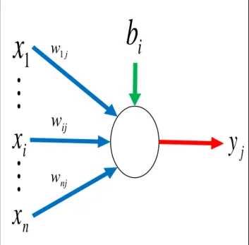
A schematic diagram of a typical j-th node is shown in Fig. 2. The inputs to such a node may come from system causal variables or outputs of other nodes, depending on the layer that the node is located in. These inputs form an input vector X = (x1, . . . , xi, . . . , xn). The sequence of weights leading to the node form a weight vector Wj = (w1j, . . . , wij,. . . , wnj), where wij represents the connection weight from the i-th node in the preceding layer to this node.
Fig. 2 Schematic Diagram of Node j
The output of node j is obtained by computing the value of the activation function with respect to the inner product of vector X and Wj minus bj, where bj is the threshold value, also called the bias, associated with this node, i.e.:
(
j j)
j
f
X
W
b
y
'=
.
−
(1) where function f (.) is the activation function, whose functional form determines the response of a node to the total input signal it receives. The most commonly used form of f (.) is the sigmoid function, given as:
t
e
t
f
−+
=
1
1
)
(
(2) The sigmoid function is a bounded, monotonic, non-decreasing function that provides a graded, nonlinear response. This function enables a network to map any nonlinear process. The popularity of the sigmoid function is partially attributed to the simplicity of its derivative that will be used during the training process.1
x
i
x
n
x
j
y
i
b
jw
1 ijw
njw
. . .
.
. .
. . .
Network InputX
Network OutputY
Input Layer Hidden Layer Output LayerB. Network Training
In order for an ANN to generate an output vector that is as close as possible to the target vector, a training process, also called learning, is employed to find optimal weight matrices W and bias vectors b, that minimize a predetermined error function that usually has the form:
(
)
∑∑
= =−
=
p j n i j i j iy
y
E
1 1 2 ' , , (3) In Equation (3), yi,jis the observed (i.e. the target) i-thelement of the j-th output variable,
' ,j i
y
is the corresponding value predicted by the model, p is the number of output variables (i.e. the number of output nodes) and n is the number of observations for each output variable. In general, there are two types of training: the supervised and un-supervised.
C. Supervised Training Algorithm
A supervised training algorithm requires an external teacher to guide the training process. This typically implies that a large number of examples (or patterns) of inputs and outputs are required for training. The inputs are cause variables of a system and the outputs are the effect variables. This training procedure involves the iterative adjustment and optimization of connection weights and threshold values for each of nodes until the error function in Equation (3) is minimised by searching for a set of connection strengths and threshold values that cause the ANN to produce outputs that are equal or close to targets. After training has been accomplished, it is hoped the ANN is then capable of generating reasonable results given new inputs.
Back-propagation is perhaps the most popular algorithm for training ANNs [8]. It is essentially a gradient descent technique that minimizes the network error function in Equation (3). Each input pattern of the training data set is passed through the network from the input layer to the output layer. The network output is compared with the desired target output, and an error is computed based on Equation (3). This error is propagated backward through the network to each node, and correspondingly the connection weights are adjusted based on Equation (4):
)
1
(
.
)
(
+
∆
−
∂
∂
−
=
∆
w
t
w
E
t
w
ij ij ijε
α
(4) where ∆wij(t) and ∆wij(t - 1) = weight increments between node i and j during the tth and (t -1)th pass, orepoch. ε and α are called learning rate and momentum,
respectively.
A similar equation is written for correction of bias values. The momentum factor can speed up training in very flat regions of the error surface and help prevent oscillations in the weights. The learning rate is used to increase the chance of avoiding the training process being trapped in a local minimum instead of the global minima. The above assumes that the architecture of the network, i.e. the number of hidden layers and nodes/layer, is known. However, this is not true and the best architecture has to be established as
part of the training process. In general, it has been shown that one hidden layer such as that in Fig. 1, having sufficient number of neurons, can approximate any complex relationships and thus most ANNs comprise one hidden layer. The number of neurons in this single hidden layer is determined by trial and error [9].
D. Unsupervised Training Algorithm
In contrast to supervised training algorithms, an unsupervised training algorithm does not involve a teacher. During training, only an input data set is provided to the ANN that automatically adapts its connection weights to cluster those input patterns into classes with similar properties. The most commonly used unsupervised ANN is the Kohonen self-organising map shown in Fig. 3 [10]. It is usually presented as a dimensional grid or map whose units (i.e. nodes or neurons) become tuned to different input data patterns.
Fig. 3 Illustration of the winning node and its neighbourhood in the Kohonen Self-organizing Map
The principal goal of the KSOM is to transform an incoming signal pattern of arbitrary dimension into a two-dimensional discrete map in such a way that similar patterns are represented by the same output neurons, or by one of its neighbours [11]. In this way, the KSOM can be viewed as a tool for reducing the amount of data by clustering, thus converting complex, nonlinear statistical relationship between high dimensional data into simple relationship on low dimensional display [10, 12]. This mapping roughly preserves the most important topological and metric relationship of the original data elements, implying that the KSOM translates the statistical dependences between the data into geometric relationships, whilst maintaining the most important topological and metric information contained in the original data. Hence, not much information is lost during the mapping. In addition, similarities in relationship within the data and clusters can be visualised in a way that enables the user to explore and interpret the complex relationship within the data set.
Kohonen Map
(Low-Dimensional Space)
Winning Node
Neighbourhood
Neurons
(Nodes)
Mapping
Input Vector
(High Dimensional
Space)
(
)
KSOM algorithms are based on unsupervised competitive learning, which means that training is entirely data driven and the neurons or nodes on the map compete with each other. In contrast to supervised ANNs, which require that target values corresponding to input vectors are known, KSOM does not require the desired output to be known, hence, no comparisons are done to predetermine the ideal responses. During training, only input patterns are presented to the network which automatically adapts the weights of its connections to cluster the input patterns into groups with similar features [13, 14].
Thus, the KSOM consists of two layers: the multi-dimensional input layer and the competitive or output layer; both of these layers are fully interconnected as illustrated in Fig. 3. The output layer consists of M neurons arranged in a two-dimensional grid of nodes. Each node or neuron i (i = 1, 2, …, M) is represented by an n-dimensional weight or reference vector Wi= [wi1,….,win]. The weight vectors of the KSOM form a codebook. The M nodes can be ordered so that similar neurons are located together and dissimilar neurons are remotely located on the map.
To train the KSOM, the multi-dimensional input data are first standardized by deducting the mean and subsequently dividing the results by the corresponding standard deviation. Each of the M nodes of the map is seeded with a vector of randomly generated standardised values; the dimension of these weight vectors is equal to that of each of the input vector. Then a standardized input vector is chosen at random and presented to each of the individual map nodes or neurons for comparison with their code vectors in order to identify the code vector most similar to the presented input vector. The identification uses the Euclidian distance, which is defined in Equation (5):
(
x
w
)
k
M
D
m v k v k;
1
,
2
,...,
1 2 ,=
−
=
∑
= ν (5)where Dk is the Euclidian distance between the current input vector and the weight vector k; m is the dimensionality of the input vector; xv is the vth element of the current input vector; wk,v is its corresponding value in weight vector k; and M is the total number of neurons in the KSOM.
The neuron whose vector most closely matches the input data vector (i.e. for which the Dk is a minimum) is chosen as a winning node or the best matching unit (BMU) as illustrated in Fig. 3. The vector weights of this winning neuron and those of its adjacent neurons are then adjusted to match the input vector using an appropriate algorithm, thus bringing the two vectors further into agreement. It follows that each neuron in the map internally develops the ability to recognize input vectors similar to itself. This characteristic is referred to as self-organizing, because no external information is supplied to lead to a classification [15].
The process of comparison and adjustment continues until some specified error criteria are attained when the training stops. The following two error criteria are normally used: the quantization error and the topological error
defined by Equations (6) and (7), respectively [16, 17]. Ref. [16] provided further details regarding the step-by-step procedure of the KSOM algorithms, including particular descriptions of the weight updating and neighbourhood functions.
∑
=−
=
N c ex
W
N
q
11
λ λ (6)∑
==
N eu
x
N
t
1)
(
1
λ λ (7)where qe is the quantization error; N is the number of samples; Xλ is the λth data sample or vector; Wc is the prototype vector of the best matching unit Xλ denotes Euclidian distance; te is the topological error; and u is a binary integer, which is equal to 1, if the first and second best matching units for the argument of u are not adjacent units on the map, otherwise u is zero.
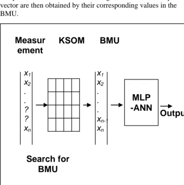
The application of the KSOM for prediction purposes is illustrated in Fig. 4 [18]. First, the model is trained using the training data set. Then to predict a set of variables as part of an input vector, they are first removed from the vector and the depleted vector is subsequently presented to the KSOM to identify its BMU using the Euclidian distance calculated with the depleted input vector, i.e. any missing variable is just omitted from the calculation of the relevant Dk. However, since the code vector of the identified BMU is complete, the values for the missing variables in the input vector are then obtained by their corresponding values in the BMU.
Fig. 4 Diagrammatic representation of the integrated KSOM-ANN modelling strategy
The KSOM can be used for many practical tasks, such as the reduction of the amount of training data for model identification, nonlinear interpolation and extrapolation, generalisation and compression of information for easy transmission [10, 19]. Indeed, the KSOM has been used for a
x1 x2 . . ? ? xn
Measur
ement
KSOM
Search for
BMU
x1 x2 . . . xn-1 xnBMU
MLP
-ANN
Output
wide variety of applications, mostly for engineering problems but also for data analysis [20]. However, the most important applications of the KSOM have been in the visualisation of high-dimensional systems and process data and the discovery of categories and features in raw data. This application is called the exploratory data analysis or data mining [10, 19].
E. Hybrid Modelling Strategy
The formulation of the BP-ANN presented earlier assumes that all the input and output exemplars used for the training are complete, i.e. there are no missing values. If any of the vectors are incomplete, then that vector will have to be removed from the training data set thus depleting the amount of experience available to the ANN to learn from. Apart from missing values, data on environmental systems can also contain outliers, which are observations that do not belong to the population being analysed either because they are abnormally too high or abnormally too low. Where there is evidence that certain observations are outliers, such data must be removed from the record so as not to distort the subsequent analysis and the interpretation of the ensuing results. Removing outliers in this way further depletes the available data for model training. However, the KSOM could be used to pre-process the incoming information in order to remove any noise in the data record caused by missing values and outliers. Because the KSOM clusters the incoming vectors, the resulting features are complete with no missing values. Additionally, since the input vectors clustered in a given KSOM node are represented by the weight vector of that node, outliers and other unrepresentative are no longer present. In this way, the features should perform better when fed as input into a BP-ANN than using the raw input vectors. The combination of KSOM and BP-ANN is what has been presented as the hybrid modelling approach in this work and is illustrated in Fig. 4.
II. METHODS AND MATERIALS A. Case Study
The methodology of this research work was applied to data from Seafield wastewater treatment plant in Edinburgh, UK for the purpose of predicting the effluent 5-day biochemical oxygen demand (BOD5), for assessing the performance of primary clarifier of wastewater treatment works. In the application, two situations were investigated: using the MLP-ANN on raw data; and using MLP-ANN on features extracted using the KSOM (i.e. the hybrid KSOM-ANN).
The Seafield plant is part of the Almond Valley and Seafield project, an environmental regenerating initiative by Scottish Water for Edinburgh city and Lothian regions. The plant is operated by Veolia Water under a private finance initiative. The population equivalent (pe) of the treatment plant is currently 480, 000 but is predicted to increase to 520, 000 by 2023 [21].
The catchment served by Seafield treatment works contain both separate and combined sewerage systems with a number of combined storm overflows discharged to local watercourses. The main outfall, however, is situated adjacent to the proposed multimillion pound housing, leisure, business and continental ferry development at Leith Docks, and to Portebello beach in the east of the city, which has been designated a bathing beach. For the latter reason, part of the effluent of the works is subject to UV disinfection during the summer bathing season prior to being discharged.
The plant comprises 8 circular sedimentation tanks, 4 rectangular non-nitrifying aeration lanes, and 8 circular final settlement tanks. The main treatment is preceded by six screens (spacing: 6 mm), four Detritor grit removal units and four storm tanks; the storm tanks come into operation when the flow reaching the works exceeds the 3DWF (Dry weather flow) design flow. When the storm tanks fill up, they spill and this spilled flow is discharged directly into the receiving environment without any further treatment; anything left in the storm tank at the end of the storm is returned to the head of the primary tanks for treatment. A layout of the Seafield works is shown in Fig. 5.
B. Data
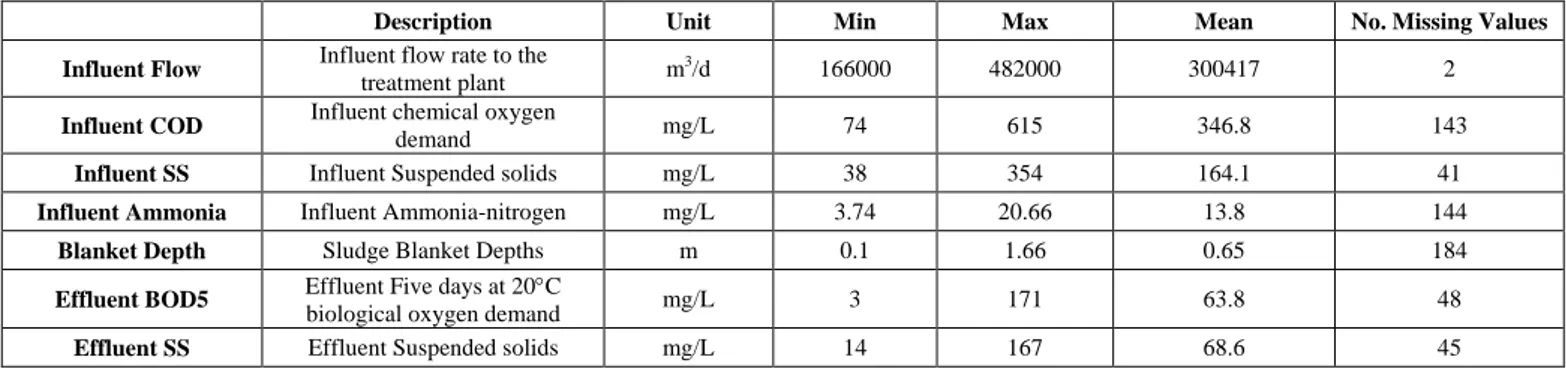
Daily record sheets describing the operation of the Seafield activated sludge treatment plant in Edinburgh (Scotland, UK) for a period of approximately three years (1 May 2002 – 31 March 2005) with a total of 1066 data vectors were obtained from the plant operators, Thames Water. A summary of the variables measured at the inlet to the works is shown in Table 1. An important feature of the data record is the large number of missing values.
Fig. 5 Layout of Seafield wastewater treatment plant: 1 is the screen house, 2 are the detritors, 3 Grit washing mechanism, 4 sedimentation tanks, 5 storm tanks, 6 aeration tanks, 7 final settling tanks, 8 UV treatment unit, 9
TABLE I WATER QUALITY CHARACTERISTICS OF THE PRIMARY CLARIFIER DATA
Description Unit Min Max Mean No. Missing Values
Influent Flow Influent flow rate to the
treatment plant m
3/d 166000 482000 300417 2
Influent COD Influent chemical oxygen
demand mg/L 74 615 346.8 143
Influent SS Influent Suspended solids mg/L 38 354 164.1 41
Influent Ammonia Influent Ammonia-nitrogen mg/L 3.74 20.66 13.8 144
Blanket Depth Sludge Blanket Depths m 0.1 1.66 0.65 184
Effluent BOD5 Effluent Five days at 20°C
biological oxygen demand mg/L 3 171 63.8 48
Effluent SS Effluent Suspended solids mg/L 14 167 68.6 45
C. Numerical Analysis and Modelling
The SOM toolbox for Matlab 5 [22] was used for the KSOM training and to extract the features. The training of the MLP-ANN used the ANN toolbox in Matlab. The neural networks have fife input variables: influent flow, influent chemical oxygen demand (COD), influent suspended solids (SS), influent ammonia, and the sludge blanket depth in the PC. These variables were chosen because of their relatively high correlation coefficients with the PC effluent BOD5 as demonstrated by Ref. [23]. To overcome the over-fitting problem, the early-stop rule was used. Since the goal of the network training is not to learn the exact representation of the training data itself but to build a model of the process that generates the data, it is important that the network exhibits good generalisation. Early stopping is the most widely used technique to overcome the over-fitting problem and to find the network having the best performance on new data. Early stopping involves the splitting of the available data into 3 subsets: training set, validation set and testing. During network training, the error on the validation set is monitored as well as the error on the training set. Training will continue until the error on the validation set increases implying over-fitting [7, 8]. Training can therefore be stopped at the point of the smallest error with respect to the validation data set, since this gives a network that is expected to have the best generalization performance. After the model has been trained, the testing set is then used to verify the effectiveness of the stopping criterion and to estimate the expected performance in the future [9]. In the current study, the split adopted was as follows: for training (500 data points); for validation (200 data points); and for testing (366 data points). All the models were evaluated using three criteria namely, correlation coefficient (R), mean square error (MSE) and average absolute error (AAE).
III.RESULTS AND DISCUSSION A. KSOM Component Planes
The KSOM component planes of the features are illustrated in Fig. 6. These visualizations present large amounts of detailed information in a concise and summary manner in order to give a qualitative idea of the properties of the data. Additionally such visualizations enable the human visual system to detect the complex relationships in a multidimensional data. Each component plane shows the distribution or spread of values of one weight vector component. By comparing patterns in identical positions of
the component planes, it is possible to reveal correlations, e.g. if large (or small) values of one variable are associated with large (or small) values of another, then there is positive correlation between the two.
Each component plane can be thought of as a “sliced” version of the SOM, because it consists of the values of single vector variable in all map units. These planes are built using colour levels to show the value of a given feature of each SOM unit in the two dimensional lattice, such that the lighter the colour, the higher the relative component value of the corresponding weight vectors. In other words, the component planes show the value of the variables in each cluster [22].
Fig. 6 the SOM Component Planes
The beauty of the component planes is that the correlations between the components can be readily visualized. For example, there appears to be a negative correlation between the influent flow rate and the effluent BOD5 and SS concentrations, because high flow rates are associated with low concentrations of the two water quality parameters. The Edinburgh works receives combined sewage; the increased flow rate associated with storm water input will cause a dilution of the water quality parameters causing concentrations to decline. However, increased flow rate also means lower residence time in the PC and hence lower removal efficiency, which should manifest itself as increased concentrations of the SS and BOD5 in the effluent. The fact that lower effluent concentrations of these water quality parameters are being observed here is probably because the effect of the dilution has exceeded the effect of the reduction in removal efficiency caused by the low detention time. Another correlation visually evident from the component planes is the positive correlation between the influent flow rate and the surface & weir overflow rates, as expected. Both the surface and weir overflow rates show a
negative correlation with the effluent BOD5 and effluent SS, principally because of the dilution effect as explained earlier. Another feature is that there is clear correlation between the influent BOD5 and SS concentrations and their corresponding effluent concentrations, as one would expect a “low in, low out” relationship for these quality parameters. The estimated correlations between the variables of the
prototype vectors are presented in Table 2, which help to confirm the observations made previously by visualizing the component planes. As seen in the Table, the effluent BOD5 and SS concentrations are reasonably well correlated with all the other variables. This implies that all the other variables can be selected as causal factors when developing intelligent models for predicting the PC effluent BOD5 and SS.
TABLE II CORRELATION MATRIX FOR THE PROCESS VARIABLES
Influent Flow Influent COD Influent SS Influent Ammonia Blanket Depths Effluent BOD5 Effluent SS g/l) Influent Flow 1.00 Influent COD -0.78 1.00 Influent SS -0.73 0.95 1.00 Influent Ammonia -0.95 0.87 0.82 1.00 Blanket Depth 0.04 0.13 0.08 0.10 1.00 Effluent BOD5 -0.40 0.63 0.51 0.53 0.63 1.00 Effluent SS -0.33 0.48 0.46 0.45 0.46 0.81 1.00 B. Mlp-Ann Modelling
To reach the suitable network architecture for the MLP-ANN, simulations were run for various assumed numbers of hidden neurons. Table 3 summarizes the errors during training, validation and testing for the MLP-ANN modelling of both data sets, i.e. raw data and features of the raw data. From Table 3, it is clear that the hybrid approach involving the use of SOM features as input to the MLP-ANN performed much better than using the raw data for developing the MLP-ANN. For example, using the correlation coefficient in Table 3 to illustrate, the minimum correlation during testing for the hybrid model was 0.84 which was much higher than the maximum correlation recorded for raw data of 0.73. This same trend can be seen
for MSE and AAE, the other two error criteria evaluated where in general the AAE for the raw data is generally twice as large as the corresponding value for the hybrid model for all the simulations. This is because the features have eliminated the noise in the raw data set, which affected the performance of the basic ANN.
Based on the summary in Table 3, the 18-node architecture can be taken as a compromise best structure since no significant improvement in all the three performance criteria occurs when the number of neurons is increased beyond 18. On the other hand, there were sustained, distinct improvements in the model performance until the 18-node structure was attained.
TABLE III RESULTS FOR THE MLP-ANN MODELS FOR PREDICTING THE PC EFFLUENT BOD5 Number
of Hidden Neurons
Data Type (Training/Validation/Testing)
Correlation % MSE AAE
Features Measured Features Measured Features Measured
3 Tr. 93 71 155.0 561.87 9.88 18.95 Va. 92 70 78.14 248.24 6.59 12.39 Te. 94 71 73.11 270.55 6.81 13.15 5 Tr. 90 64 529.4 802.33 18.5 22.20 Va. 91 68 133.3 248.12 9.30 12.42 Te. 98 61 135.1 341.22 9.12 15.00 7 Tr. 96 77 145.2 476.17 9.42 17.45 Va. 94 72 66.06 237.05 5.99 12.14 Te. 96 70 89.57 273.22 7.66 13.27 10 Tr. 97 78 64.93 443.58 6.23 17.00 Va. 95 71 44.23 262.42 5.08 12.64 Te. 96 71 42.86 267.33 5.10 13.02 12 Tr. 97 79 68.49 417.76 6.42 16.22 Va. 95 71 44.45 258.39 5.12 12.62 Te. 96 71 49.04 261.77 5.55 12.89 14 Tr. 94 79 135.2 409.40 9.12 16.23 Va. 91 72 74.76 275.03 6.75 12.69 Te. 91 72 99.12 259.82 8.02 12.87 16 Tr. 92 80 659.5 406.66 20.5 16.23 Va. 86 71 204.4 258.27 11.4 12.14 Te. 84 71 183.0 264.11 10.8 12.82 18 Tr. 97 81 66.86 384.84 6.37 15.69 Va. 95 73 42.47 249.33 4.94 11.85 Te. 97 71 41.48 253.94 5.01 12.54 20 Tr. 94 80 138.4 394.62 9.47 15.70 Va. 92 73 75.74 235.47 6.79 11.60 Te. 95 73 67.71 251.23 6.40 12.73
Fig. 7 Scatter plots of the measured and predicted PC effluent BOD5 during training, validation and testing.
Fig. 8 Time series plots of the observed and predicted effluent BOD5
Fig. 9 The Residuals IV.CONCLUSION
The current work used a new methodology based on a hybrid supervised-unsupervised ANN to improve the performance of the basic back-propagation ANN method in modelling the primary clarifier of a wastewater treatment plant. The method was applied to data taken from the Seafield wastewater treatment plant in Edinburgh, UK, during a period of about three years. Input variables were selected based on their correlation with the effluent BOD5, which was the target prediction variable. Several ANN models with different numbers of neurons in the hidden layers were developed. For each model, two types of data were used, the first one is the raw data set and the second
one is the extracted features of the raw data using the Kohonen self-organising map. The results showed that the models using the features were better than those using the raw data.
The findings prove the ability of KSOM to improve the performance of modelling using basic back-propagation ANN, particularly when the available data are noisy, a common problem with the process data of wastewater treatment plants. Furthermore, the KSOM can readily deal with missing values in one or more of the input variables without significantly negative impacts on the accuracy of the model. The methodology is therefore applicable to other water and environmental engineering problems.
REFERENCES
[1] Geraney, K., Vanrolleghem, P. A. & Lessard, P. (2001) Modelling of a reactive primary clarifier. Water Sci. Technol. 43(7), 73–81. [2] Lessard, P. & Beck, M. B. (1988) Dynamic Modelling of Primary
Sedimentation. J. Environ. Engrng, ASCE, 114 (4), 753-769. [3] Otterpohl, R. and Freund, M., 1992. Dynamic models for clarifiers of
activated sludge plants with dry and wet weather flows. Wat. Sci. Tech., 26(5–6), 1391–1400.
[4] Lessard P. and Beck M.B., 1991. Dynamic modelling of wastewater treatment processes: its current status. Envir. Sci. Technol. 25, pp. 30–39.
[5] Manfred, S., Butler, D. and Beck, M. B., 2002. Modelling, Simulation and Control of Urban Wastewater Systems, 27–29. Springer-Verlag London Limited, 357.
[6] Pu, H. and Hung , Y. 1995. Artificial Neural Networks for Predicting Municipal Activated Sludge Wastewater Treatment Plant Performance , Intl. J. Environmental Studies, 48, 97 – 116.
[7] Arbib M.A, 2003. The handbook of brain theory and neural networks. 2nd ed. MIT.
[8] Abrahart R.J., Kneale P.E., See L.M., 2004. Neural networks for hydrological modelling. Publisher: Balkema.
[9] Adeloye A.J., De Munari A., 2006.Artificial neural network based generalized storage–yield–reliability models using the Levenberg– Marquardt algorithm. Journal of Hydrology, 326(1-4): 215-230. [10] Kohonen, T., Oja, E., Simula, O., Visa, A. & Kangas, J. (1996)
Engineering applications of the Self Organising Map. Proceedings IEEE, 84(10), 1358–1384.
[11] Back B., Sere K. and Hanna V., 1998. Managing complexity in large database using self-organising map. Accounting Management & Information Technologies, 8:191-210.
[12] Zhang L. , Scholz M. , Mustafa A., Harrington R, 2009. Application of the self-organizing map as a prediction tool for an integrated constructed wetland agroecosystem treating agricultural runoff, Bioresource Technology, 100(2): 559-565.
[13] Obu-can, K., Fujimura, K., Tokutaka, H., Ohkita, M., Inui, M. and Ikeda, Y., 2001. Data mining of power transformer database using self-organising map. Tottori University, Dept. Of Electrical and Electronics Engineering, Koyama-Minami, Japan. Www.ele.tottori-u.ac.jp.
[14] Astel A., Tsakovski S., Barbieri P., Simeonov V., 2007. Comparison of self-organizing maps classification approach with cluster and principal components analysis for large environmental data sets. Water Research, 41(19): 4566-4578.
[15] Penn B.S., 2005. Using Self Organizing Maps to Visualize high dimensional Data. Computer and Geoscience 31, pp. 531-544. [16] Garcia, H. &Gonzalez, L. 2004. Self-organizing map and clustering
for wastewater treatment monitoring. Eng. Appl. Artific. Intellig. 17(3), 215–225.
[17] Hong, Y., Rosen, M., Bhamidimarri, R., 2003. Analysis of a municipal wastewater treatment plant using a neural network-based pattern analysis. Water research 37, 1608-1618.
[18] Rustum R and A.J.Adeloye, 2007. Replacing outliers and missing values from activated sludge data using Kohonen Self Organizing Map. Journal of Environmental Engineering, 133 (9): 909-916. [19] Kangas. J. and Simula, O., 1995. Process monitoring and
visualization using self-organising map. Chapter 14 in (ed. Bulsari, A. B.) Neural Networks for Chemical Engineers, Elsevier Science Publishers.
[20] Badekas E., Papamarkos N., 2007.Optimal combination of document binarization techniques using a self-organizing map neural network. Engineering Applications of Artificial Intelligence, 20(1): 11-24. [21] Hill A. and Hare G, 1999. The almond valley and Seafield PFI
project risk issues associated with flow prediction. WaPUG Autumn Meeting, 1999.
[22] Vesanto, J., Himberge, J., Alhoniemi, E. & Parhankangas, J. (2000) Self-organizing map (SOM) Toolbox for Matlab 5. Report no. A57, Laboratory of Computer and Information Science, Helsinki University of Technology, Helsinki, Finland.
[23] Rustum, R. & Adeloye, A. J. (2006) Features extraction from primary clarifier data using unsupervised neural networks (Kohonen Self Organising Map). In: 7th International Conference on Hydroinformatics, HIC 2006, Nice, France.
Rabee Rustum, civil and environmental engineer specializing in hydroinformatics with experience in water and wastewater related projects. Dr. Rustum graduated with BSc (First Class) degree from Damascus University, Syria in 2001. After graduation, he worked as an environmental engineer for the Water Pollution Control Department, Ministry of Irrigation, Syria. In 2002, he got a Post Graduate Diploma (First Class) in Civil and Environmental Engineering from Damascus University, Syria; and in 2003 he obtained a Master’s Degree in environmental risk management from Poitiers University, France. Dr. Rustum started his research career in 2005 and in June 2009 he obtained his PhD in Civil & Environmental Engineering from Heriot-Watt University, Edinburgh, United Kingdom. From June 2008, he worked as a water and wastewater hydraulic modeller for Mouchel Group, Stirling office, Scotland, UK. In September 2009, he joined King Faisal University, Dammam, Saudi Arabia as assistant professor in environmental engineering before joining the water research group at Heriot-Watt University.
Adebayo Adeloye, graduated with BSc (First Class, First Position) degree from the University of Ife (now Obafemi Awolowo University, Ile-Ife), Nigeria in 1977, specialising in irrigation and soil and water engineering. After a stint in consulting practice, he went on to obtain the MSc and PhD degrees at the University of Newcastle upon Tyne, UK, specialising in Water Resources engineering and management. In 1987, Dr Adeloye won the prestigious and highly competitive Fellowship of the Royal Commission for the Exhibition of 1851, a post-doctoral fellowship tenable at the Imperial College of Science, Technology and Medicine, London. Dr. Adeloye joined Heriot-Watt University as a lecturer in 1992 and was promoted to a Senior Lecturer in 2004. He is the co-author of “Water Resources Yield”, a postgraduate reference textbook first published in 2005 by Water Resources Publications, Colorado, USA. In addition to being a chartered engineer, and a chartered water and environmental manager, Dr Adeloye is also currently a Fellow of the Higher Education Academy.