In Finance, Size Matters:
The “Systemic Scale Economies” Hypothesis
BIAGIO BOSSONE and JONG-KUN LEE*
This study investigates the relationship between production efficiency in financial intermediation and financial system size. The study predicts and tests for the exis-tence of “systemic scale economies” (SSE) effects, whereby value-maximizing inter-mediaries operating in large systems are expected to have lower costs of production, risk absorption, and reputation signaling than intermediaries operating in small sys-tems. The study explores the mechanics of SSEs and estimates their quantitative relevance using a large cross-country banking data panel. The study shows strong evidence in support of SSEs and finds that the institutional environment, risk envi-ronment, and market concentration affect significantly the production efficiency of financial intermediation services. [JEL D21, G14, L16]
I
n this study we formulate and test empirically what we call the “systemic scale economies” (SSE) hypothesis, whereby the production of financial intermediation services shows increasing returns in the scale of the system where it takes place. Noting that financial intermediaries are nowadays more and more integrated in infrastructural networks of various kinds, we argue that the efficiency of financial intermediation should reflect, inter alia, the efficiency of the networks supporting their activity. In this sense we can speak of systemic scale effects.In simple words, our hypothesis holds that an intermediary of any given size operating in a large domestic financial system should be expected to be more © 2004 International Monetary Fund
*Biagio Bossone is Executive Director of the World Bank for Albania, Greece, Italy, Malta, Portugal, San Marino, and Timor-Leste, and is also associated with the Banca d’Italia. Jong-Kun Lee is Head, Macro-economic and Quantitative Studies Team at the Institute for Monetary and Economic Research, Bank of Korea. The authors wish to thank G. Dell’Ariccia, R. Flood, A.-M. Gulde, G. Majnoni, J. Hanson, P. Honohan, and two anonymous referees for their helpful comments.
cost-efficient than the same intermediary (hypothetically) operating in a smaller system, all else being equal. If this hypothesis is established empirically, its main implication is that intermediaries in small financial systems face greater (structural) challenges in achieving market viability than those in larger systems. This issue and its policy reflections are discussed in a World Bank study on the economic costs associated with small size in finance (see Bossone, Honohan, and Long, 2001).
This study investigates the existence of SSEs in banking intermediation using state-of-the-art cost analysis techniques on a cross-country and time-series bank data panel in the context of a model where intermediaries are assumed to maxi-mize value, rather than profits, and therefore are sensitive to both first and second moments of their profit distribution function.
I. Scale Efficiency in Finance: What We Already Know
Significant scale economies exist at the level of individual intermediaries and infrastructural systems. The following is a short review of the empirical literature on the subject. It draws on the much more extended review contained in Bossone and Lee (2002).
Scale Efficiency in Financial Intermediation
Although economies of scale are integral to the theory of financial intermediation, empirical research has failed for a long time to support the theory’s predictions. Recent studies on banking, however, have uncovered strong scale effects (Berger, Demsetz, and Strahan, 1999) and have found that size has efficiency implications also for risk-management and reputation-signaling activities.1,2
Hughes and Mester (1998) detect large economies of scale across all bank sizes and show that, as scale increases, banks economize on the financial capital used to cushion risks and to signal strength to the market and save on the costs of the (labor and physical capital) resources employed to manage risks and to preserve financial capital. Hughes and Mester also find scale economies in reputation signaling (prox-ied by the marginal cost of financial capital), which their evidence shows to be sig-nificantly lower in the largest banks.
Other studies show that scale efficiency gains derive also from the geographical diversification of risk. In the United States, the change in scale efficiency reflects the 1A larger scale may enhance the potential for risk diversification through a wider mix of financial prod-ucts and services supplied, as well as via increased geographic spread of activities. McAllister and McManus (1993) first showed that the standard deviation of the rate of return on U.S. bank loans declined rapidly as bank loan portfolios approached US$1 billion in size. However, scale economies from risk diversification may be hidden by the banks’ response to a reduced marginal cost of risk by taking on more risk in exchange for higher expected returns (Chong, 1991; Demsetz and Strahan, 1997). Thus, as lower asset quality requires more resources to manage the extra risk, measured scale economies may appear to be lower if the change in asset quality is not controlled.
2Studies of the U.S. banking industry find scale economies on the order of 20 percent of costs for bank sizes up to about US$10 to US$25 billion in assets (Berger and Mester, 1997) and, contrary to earlier evi-dence, observe that scale economies increase with the size of banks (De Young, Hughes, and Moon, 1998; Hughes, 1999).
elimination in 1985 of the geographic restrictions on the expansion of bank branch-ing and bank holdbranch-ing companies, which until then had precluded smaller banks from achieving larger and more efficient sizes (Calem, 1994). Hughes and others (1999a) find that the more geographically diversified U.S. bank holding companies have lower deposit volatility, higher expected returns, and lower risk. Hughes and others (1999b) confirm the benefits of geographic diversification using a model that incor-porates market value information on banks.3
Evidence of significant scale economies in banking is found across European banking systems,4in Japan (Fukuyama, 1993), Australia (Walker, 1998), and India (Das, 1998), while no evidence (at least, to our knowledge) has been systematically collected and evaluated for banking institutions in small or very small countries, or on a consistent cross-country basis, which would indirectly show the effects of sys-tem size on bank efficiency levels (syssys-temic scale effects).
Scale Efficiency in Financial Infrastructure
Recent studies confirm that infrastructures such as payment systems and organized securities markets have increasing returns to scale. Hancock, Humphrey, and Wilcox (1999) find significant economies of scale in payment system data processing. They report the results from studies of the cost structure of the Automated Clearing House (ACH) electronic transfers in the United States and cite evidence from a study of the Federal Reserve’s electronic book-entry government securities transfer system (Belton, 1984). Payment systems are characterized also by network externalities (Saloner and Shepard, 1995; Gowrisankaran and Stavins, 1999).
As regards organized securities markets, evidence supports the existence of significant scale efficiency effects both in trading operations and in firm-specific information processing activities (listing) and indicates that cost-effectiveness of stock exchanges is higher where regulation is more homogeneous (Malkamäki, 1999; Hasan and Malkamäki, 2001). Stock exchange transaction costs decline sharply relative to the transaction value as the size of transaction grows, even in advanced markets (Green, Maggioni, and Murinde, 2000). Network effects, too, are present in organized markets (Cybo-Ottone, Di Noia, and Murgia, 1999).
Finally, there are indications that scale economies characterize regulatory sys-tems as well. Country survey data on the cost to the public authorities of providing banking regulation and supervision indicate that such costs increase less than pro-portionately with the size of the system (Bossone, Honohan, and Long, 2001).
3Their analysis shows that, with constant asset size and branch networks, an increase in deposit dis-persionacross states is associated with lower insolvency and profit risks; that macroeconomic diversifica-tionis negatively related to both profit risk and insolvency risk; that extensivenessof the branch network improves bank profits and lowers insolvency risk; and that a proportional increase in assets, branches, deposit dispersion, and macro diversification increases more than proportionally the market value of bank equities and assets. The authors conclude that the “benefits of geographic expansion and diversification give banks an important economic incentive to consolidate, especially across state lines” (p. 317).
4See Bossone and Lee (2002) for a comprehensive list of references and an illustration of the main results.
II. Scale Efficiency in Finance: What We Want to Know
The literature on scale economies in finance suggests that production efficiency in financial intermediation should reflect not only the production scale of the individ-ual intermediary, but also the size of the financial system where the intermediary operates (the SSE hypothesis). Some of the studies reviewed, in particular, place special emphasis on scale efficiency effects relating to risk-management functions. This section identifies the channels through which the size of the financial system may affect production and risk-management efficiency in financial inter-mediation and formulates two testable propositions. Due to data availability, our empirical analysis focuses on bank production. However, in our view there is no specific reason why the results of the analysis should not be generalized to non-bank financial intermediaries.
Identifying and testing SSE channels builds on the new literature on scale economies in bank production (reviewed in Section I) since the path-breaking con-tribution by McAllister and McManus (1993).5Two features from this literature are crucial to our study: first, risk taking in bank production is endogenous; and second, banks maximize value (rather than profits).
As regards the first feature, the estimation of bank scale efficiency must con-trol for the impact of endogenous risk decisions on costs: if an increase in system size reduces the marginal cost of risk taking for individual banks, and hence raises the banks’ marginal return on risk taking, the banks have an incentive to take on additional risks, that is, to reduce their asset quality in the expectation of higher returns. However, since higher risks generate additional risk-management costs (including higher financial capital, more inputs, and higher risk premiums on bor-rowed funds), the banks may actually use up (part of ) the initial cost savings. As a result, estimates that did not duly account for risk endogeneity would not capture the full cost effects of scale.
As for the bank objective function, the profit-maximization (cost-minimization) objective assumed in the standard models used to measure bank production effi-ciency may be inappropriate. Since risks create the potential for costly episodes of financial distress, banks seek to maximize value and are prepared to trade higher profit for lower risk. By incorrectly assuming profit maximization, standard mod-els may fail to detect the responsiveness of the bank risk /return trade-off to scale effects: bankers may find the level of financial capital implied by profit to be un-acceptably low. Their demand for capital would have to be modeled by a broader objective than profit maximization.6However, high market concentration or too-large-to-fail types of expectations may reduce the perceived riskiness of individual banks (at least of the dominant ones) and weaken their incentive to accumulate financial capital in the face of given risks. Failing to control for market concentra-tion would therefore lead to biased estimaconcentra-tions of systemic scale externalities.
5As recalled, McAllister and McManus showed that the standard deviation of the rate of return on bank loan portfolios falls dramatically as the size of the portfolios increases up to a level, presumably due to diversification effects. Such risk reduction lowers the amount of physical and financial resources that banks need to manage their risk exposures.
6For a thorough discussion of these issues and their applications, see Hughes and Mester (1998), Hughes and others (2001), and Hughes (1999).
Both these aspects are incorporated in the methodology used in the next section to test the SSE hypothesis. This hypothesis can be translated into the following two operational propositions.
Proposition 1: SSEs in Production.All else being equal, banks operating in larger financialsystems have relatively lower production costs than banks operating in smaller systems.
If the scale efficiency effects incorporated in financial infrastructural services feed back into bank production (independently of the bank-specific production cost structure), the average production cost should be expected to be higher (lower) for banks operating in small (large) systems and to decrease with the size of the finan-cial system where the banks operate. As an example, a larger payment system or a larger infrastructure for the dissemination of financial information should offer less expensive (implicit or explicit) service charges to accessing banks, thereby afford-ing banks lower production costs.
Also, since banks need to raise their financial capital when expanding produc-tion, larger financial systems should allow them to economize on capital resources by diversifying their asset portfolio more efficiently across a broader borrower base and over a wider spectrum of activities and geographic areas. An increase in the output of banks operating in larger systems should thus require proportionately less financial capital than that of banks in smaller systems.
Finally, the cost structure of the banks should be expected to change differ-ently over time, in response to changes in the technology embodied in financial infrastructure, depending on the size of the financial system in which they oper-ate. Banks operating in larger financial systems should benefit more rapidly from technological developments that improve the efficiency of infrastructural ser-vices used as production inputs.7This effect should be measured by observing a more (less) rapid pace of cost decline for banks operating in larger (smaller) sys-tems. The more rapid decline would be caused by the interaction between net-work externalities and scale economies that typically characterize infrastructural network services.
The types of SSEs in production just discussed derive from the absolutescale of the financial system (as opposed to the SSE effects associated with the size of the financial system relativeto that of the economy—see Proposition 2 below). Therefore, a levelvariable should be used in an empirical cross-sectional compar-ative analysis. This level variable should also include information on the degree of openness of the system to international transactions, as this would reflect the extent to which the domestic financial system is integrated into (wider) inter-national financial infrastructural networks.
7When the same technology development takes place in two network systems that hypothetically dif-fer in size only, the network externalities in the larger system are stronger because the larger size attracts more users; more users mean larger economies of scale and lower service charges, which in turn generate additional network economies. The reduction in production cost and service charges per time unit would be larger in the larger system.
Proposition 2: SSEs in Risk Management.All other things being equal, banks that operate in larger (deeper and more efficient) financialmarkets have relatively lower costs of risk absorption and reputation signaling than banks operating in smaller financial markets.
Banks use financial capital as a buffer against risks and as a device to signal their financial soundness to the market. As Hughes and Mester (1998) note, given the observable scale and asset quality of a bank, an increase in its financial cap-ital reduces the likelihood of insolvency and provides an incentive to allocate addi-tional resources to risk-management activities aimed at protecting the larger equity stake. A higher degree of capitalization (for given observable scale and asset qual-ity) also signals the greater safety of the bank and enhances its market reputation. In competitive markets, therefore, banks need to accumulate more financial capital than if they faced less competition. Yet a bank’s demand for financial capital should be expected to grow less than proportionately than the size of the financial markets where the bank operates, for a number of reasons:
• First, deeper and more efficient financial markets help banks improve their screening of potential borrowers,8monitor their investment more efficiently, and signal their risk attitude through information other than (and possibly comple-mentary to) accumulated financial capital. As a result, banks operating in large financial markets should attain the same degree of protection against financial distress and the same reputation-signaling effect with a lower capital-to-asset ratio than those operating in smaller markets. As an implication, banks in small (large) financial markets should over- (under-) utilize financial capital.
• Second, deeper and more efficient financial markets should enable banks to manage and protect their financial capital with relatively fewer nonfinancial resources. More specifically, as banks increase their output and adjust their financial capital position accordingly, they may need to mobilize additional (nonfinancial) resources to manage and protect their financial capital. The presence of SSEs should imply that banks operating in larger financial markets perform these functions with relatively fewer nonfinancial resources than those operating in smaller markets.
• Third, with better information provision (meaning more and higher-quality information) and investors’ larger signal-extraction capacity, signaling is more efficient and banks can economize on the financial capital needed to signal a given level of reputation or risk safety. The same holds if investors can rely on greater regulatory and rule enforcement capacity.
• Fourth, with better information provision and higher signal-extraction capacity, banks operating in larger and more efficient financial markets should be able to raise new financial capital with a less than proportional increase in their costs since, all else being equal, achieving a higher level of capital would signal a stronger financial position.
8This effect rests on the assumption that banks use capital market information like other nonbank investors do. As stock markets aggregate (and reflect on prices) the views of a wide range of different investors (Allen and Gale, 1999), they provide “multiple checks” on individual firms and, hence, the best indicators possible of the true value of the firms.
Investigating empirically the SSE channels implied by Proposition 2 suggests the use of a relativesize indicator, as financial market depth and efficiency are better proxied by variables that measure the scale of the markets relative to the size of the overall economy.
Propositions 1 and 2 can be summarized by saying that larger financial systems
enable intermediaries to lower their (average and marginal) resource costs for man-aging risks, and that deeper financial marketsenable them to increase the efficiency of their risk-management capacity.
Taken together, the two propositions imply that in larger and more efficient financial systems the minimum efficient bank size should be smaller (all else being equal). The development of financial infrastructure should in principle allow all banks to gain efficiency across all classes of system size. All else equal, a reduc-tion in average producreduc-tion costs across all system size classes increases the prof-itability of all banks and induces new market entry from the set of inframarginal banks: if production at the bank level shows increasing returns relating to SSEs, small banks that were unprofitable in systems with small and inefficient infrastruc-ture would become viable once they gain access to larger and more efficient infras-tructure. They can therefore enter the market and be able to survive. Testing this third proposition could be the subject of future work.9
III. Testing the SSE Hypothesis
Testing the SSE hypothesis requires making assumptions on the behavior of the intermediaries, selecting the appropriate model for estimation, and identifying the necessary statistical information.
Model and Estimation
The bank’s value-maximizing problem is to minimize the economic cost resulting from the sum of the cash-flow cost and the opportunity cost of equity capital (k) at the time of evaluation.10,11Assuming the intermediation hypothesis, which regards deposits as inputs to production, the restricted-variable cost function (CV) is derived
from the cost minimization problem subject to the quasi-fixed input of equity cap-ital (k=k0) and risk-related asset quality (q) as a conditioning argument. In addition
9Interesting implications of this proposition are that (i) the minimum size for a bank to be viable depends on the structure (that is, scale, sector composition, and efficiency) of the financial systems where it operates, and that (ii) the economic costs of financial intermediation vary inversely with the size of the financial system. 10For bank managers who are not risk neutral, maximizing value (as against profits) implies that they are willing to trade profit for reduced risk. They therefore attribute a positive value to guarding against financial distress and the need to signal their bank’s safety by choosing a level of capitalization that likely exceeds the cost-minimizing level.
11Thus, the long-run (total) economic cost function (C
T) is specified as CT=CV+w*kk,where w*kis a
shadow price of financial capital (= −∂CV/∂k). Since it is generally difficult to obtain wkupon empirical
estimation of a long-run (equilibrium) total cost function, the shadow price of capital (w*k) has been
fre-quently used as a substitute for the market rental price of capital (wk) in the literature. Note that wk=w*k
to Hughes and Mester (1998), whose underlying model specification incorporates the risk-endogeneity effect by including the response of financial capital to changes in asset quality, we amend the short-run variable cost function, CV, by adding an
appropriate control variable (φ) for capturing country-specific financial sector fea-tures in each country observed and a proxy variable for technological progress (t). Then, CV, viewed as a cash-flow cost function, is defined as
(1) where T() = transformation function; Q = output (total loans and other earning assets); wp=price of physical inputs; wd=price of deposits (d); x =quantity of
variable factor input (=xp+xd). To estimate the conditional variable cost function
(CV), we use the translog functional form as follows:
(2)
where Z=(Q,wl, wd, wc, k,t,qa, FS,FD) and
Q: single aggregate output
VC: variable cost (= Σwjxj, j=p, d)
wj: variable factor prices for labor (l), deposits (d), and physical capital (c)
k: financial (equity) capital
t: time trend variable representing technological progress
qa: asset quality (adjusted nonperforming loan ratio =NPL / INST)
FS: (absolute) financial system size (in billions of U.S. dollars)
FD: (relative) financial system depth (FS/GDP* MS), MS=financial mar-ket size.
The variable factor share equations (Sj) and one shadow price equation (wk)
can then be derived directly from equation (2), by differentiating CVwith respect
to variable factor prices (wl, wd, wc) and quasi-fixed factor input of equity capital
(k). With symmetry (βij= βji) and linear homogeneity imposed, the derived
equa-tions are expressed as follows:
(3)
(4)
As in Hughes and Mester (1998), we explicitly specify the financial capital demand equation in order to capture the endogeneity of financial capital in asso-ciation with risk-related asset quality:
w C k Z VC k k V k ik i i = −∂ ∂ =
(
α +∑
β ln)
. Sj j ij Zi j d c Sj i = α +∑
β ln , =1, , ,∑
=1 lnVC ilnZi lnZ lnZ , i ij i j j i = α0 +∑
α +∑
∑
β 1 2 Cv Q w w k q t w x w x T Q x k q t k k p d p p d d , , , , , , min , , :, , , , φ φ ( ) = ( + ) ( ) ≤ = s.t. and 0 0(5) where
CN: banking market concentration (0 ≤CN≤1)
R: liquidity asset ratio
Π: profitability (spread between loan and deposit interest rates).
After substituting equation (5) into (2), (3), and (4), we estimate the system equations of factor demand, consisting of the restricted variable cost function (equation (2)), two share equations (out of three) for variable inputs (equation (3)),12 and the shadow price of equity capital (equation (4)). Upon empirical esti-mation, the intercept terms α0in (2) and γ1in (5) are allowed to vary across coun-tries to mitigate the heterogeneity of the underlying sample, thus enabling us to take into account country-specific differences. The model is estimated simultaneously by applying an iterative seemingly unrelated regression (SUR) estimation tech-nique. The estimates obtained are asymptotically equivalent to maximum likeli-hood estimates. The estimation results for pooled cross-section time series are not shown here,13but most of the parameter estimates are statistically significant at the 5 percent level. The R2s in the system equation regressions are high, showing an acceptable goodness of fit.14
Defining Measures of Scale Economies in Banking
Once a translog cost function is explicitly specified, we can derive parametric esti-mates of scale economies. We use four measures of scale economies (εCQ), defined
as follows. Note in the following that εCQ> 1 implies economies of scale (i.e., less
proportionate increase in C with respect to changes in Q ⇒ ∂lnC/∂lnQ < 1), whereas εCQ< 1 implies diseconomies of scale.
(1) Conventional Measure of Scale Economies in CV
When a multiproduct cost function (Q= (Q1, Q2, . . . , Qn)) is assumed, the
Conventional Measure of Scale Economies is defined as
(6)
which shows how cost changes in proportion to output variations.
εVCQ V i i n C Q = ∂ ∂
∑
1 ln ln , ln ln ln ln ln ln ln ln , k Q FS FD CN qa R = + + + + + + + ∏ γ γ γ γ γ γ γ γ 0 1 2 3 4 5 6 712Since the variable input cost-share equations sum to unity, the share equation for physical capital (Sc) was deleted from the estimated system of equations. See Berndt, Hall, and Hausman (1974) for details.
13Detailed parameter estimates are available from authors upon request.
14R2: 0.972 for variable cost equation, 0.390 for labor cost-share equation, 0.406 for deposit cost-share equation, and 0.177 for shadow price of financial capital equation. The log of likelihood functions is com-puted as 6,717.2 over 2,625 total sample observations.
(2) Quality-Adjusted Measure of Scale Economies in CV
Following Hughes and Mester (1998), the Quality-Adjusted Measure of Scale Economies is derived by holding asset quality (q) constant:
(7)
By taking into account the endogeneity of risk and financial capital, this para-metric measure will reflect the effect on cost of a proportionate variation in the levels of output and nonperforming loans taken as a proxy for risk-related asset quality; it therefore captures the full effect on cost of both output and risk changes, thus providing further insights in the differential impact of various sources of SSEs from the individual components of the denominator of equation (7).
(3) Economic-Cost Scale Economies in CT
Following Hughes and others (2001), who use a shadow valuation of finan-cial capital, the measure of the Economic-Cost Scale Economies from a shadow total cost function is given by
(8)
where CTis the economic total cost function, defined as the sum of variable cost (CV)
and the shadow cost of financial capital taken as a substitute for its market price value. (4) Economic-Cost and Quality-Adjusted Scale Economies in CT
Finally, combining equations (7) and (8) yields the new comprehensive measure of adjusted scale economies in the total cost function:
(9) which incorporates the asset-quality control feature into the total (economic) cost structure of bank production.
Data and Sources
A sample of 875 commercial banks from 75 countries was drawn mainly from the FitchIBCA’s (2000) BankScope database, which contains banking information for
εTCQ ε q VCQ q CV k = − ∂ ∂ 1 lnln , ε φ φ φ φ TCQ T p d k T p d k v p d v p d v C Q w w w k q t Q Q C Q w w w q t C Q w w k q t Q Q C Q w w k q t C k k = ∂
(
)
∂[
]
[
( )]
= ∂ ( ) ∂[
]
( )+ −∂( ∂ )(
)
[
]
=⋅
⋅
1 1 , , , , , , , , , , , , , , , , , , , , , , , , , * 1 1 1 − ∂ ∂ ∂ ∂ = − ∂ ∂ ∑
ln ln ln ln ln ln , C k C Q C k V V i i VCQ V ε εVCQ q V i V i V V i n i n C Q C k k Q C q C k k q = ∂ ∂ +∑
∂∂ ∂∂ + ∂∂ + ∂∂ ∂∂ ∑
1 ln ln ln ln ln ln ln ln ln ln ln ln .over 1,900 commercial banks with more than US$1 billion in total assets. A total sample of 875 banks was almost equally divided into three subgroups according to the reported total asset size: small banks (292 banks, smaller than US$2.4 billion), medium banks (292 banks, between US$2.4 and $8.0 billion), and large banks (291 banks, larger than US$8.0 billion). Since a complete set of variables is required for the analysis of the bank cost structure, almost half of the banking observations for which information was partially missing or misreported had to be dropped. In those cases where the necessary banking data were not available on BankScope, we referred directly to banks’ financial statements (available on their official websites) or, as an alternative or complementary source, to official reports on domestic bank-ing from national financial supervisory authorities.
In the case of missing information for some important variables in the Bank-Scope database, average values of peer-group banks in each country were used instead. To collect comparable international data from different countries, we sim-plified the data structure by aggregating variables that for some countries were not available on a disaggregated basis. The data were extracted from nonconsolidated income statements and balance sheets, ranging from 1995 to 1997.15All banking data (except quantity variables) are reported in U.S. dollars and are adjusted for CPI inflation in each respective country. The resulting data is a pooled sample of cross-sectional time series of 2,625 observations over the three years considered (i.e., 875 observations for each year).
Following the intermediation approach to estimate economies of scale in bank-ing, our main specification for the bank’s cost function is characterized by a single output and four inputs. Output (Q) is defined as the sum of total loans and other earning assets, which are measured as the average dollar amount at the end of each year; the corresponding output price (P) is calculated by dividing the total interest revenue by the inflation-adjusted total earning asset. The inputs are two nonfinancial factor inputs, labor (xl) and physical capital (xc); and two financial inputs, deposits
(xd) and financial (or equity) capital (k).
The price of labor (wl) is obtained by dividing total salaries and benefits paid
by the total number of employees. The price of physical capital (wc) is derived as
the ratio of other operating expenses, including occupancy expenses, over inflation-adjusted fixed assets (xc). Since other operating expenses reported by BankScope
include other noninterest expenses, this may lead to overestimating the actual price of physical capital. However, the data seem to be relatively consistent across coun-tries in that information disclosure and accounting standards are identical for all banks. On the other hand, the input price of deposits (wd) is obtained by dividing
total interest expenses by the total inflation-adjusted amount of deposits (xd). The
input quantity of financial capital (k) was directly obtained from the inflation-adjusted figure for equity capital reported in the balance sheets. However, since no information was available on the cost of financial capital, the return on
aver-15As our analysis required a complete data set for each financial variable included in the cost func-tion, we had to eliminate from the initial BankScope database those banks for which information was miss-ing and could not be derived otherwise. As a result, out of the complete 1993–1997 BankScope database we could draw a sample covering only the 1995–1997 period.
age equity (ROAE) and an estimate of the market rental price of capital based on the bank production function were used as proxies for the price of financial capital (wk), reflecting the opportunity cost of equity capital.
In addition to these micro, bank-specific data, macro country-specific variables were used to control for the effects of various financial sector structural character-istics and for the different level of financial sector development in each country. The information was mainly obtained from the World Bank’s Global Development Finance(2001a, hereafter GDF ) and World Development Indicators(2001b, here-after WDI ), the IMF’s International Financial Statistics(IFS), and the databases from Beck, Demirgüç-Kunt, and Levine (1999, hereafter BDL) and from La Porta and others (1997 and 1998, hereafter LLSV).
As for the absolutesize of the financial system of each country (FS), we con-structed a comprehensive indicator for open economies by summing domestic credit, domestic deposits, foreign assets, and foreign liabilities of the banking sys-tem, expressed in billions of U.S. dollars.16We then divided the overall 75-country sample into three financial system size subgroups:17small systems (FS< US$35 bil-lion, 24 countries), medium systems (US$35 billion < FS< US$300 billion, 25 coun-tries), and large systems (FS> US$300 billion, 23 countries).
To capture the relative size of the financial system, we used the FD ratio (=FS/GDP) as a proxy for financial depth. We also constructed a composite size indicator of domestic capital markets (MS) by multiplying the three stock market ratios reported in BDL (1999): stock market capitalization to GDP (size), stock market total value traded to GDP(activity), and stock market turnover to GDP
(efficiency).18
Finally, we constructed a composite index of institutional variables (INST), including accounting standards, contract enforcement, rule of law, regulation, qual-ity of bureaucracy, and property rights from LLSV (1998), and level of corruption from Knack and Keefer (1995).19In order better to capture the different asset qual-ity of banks across sample countries, we used the ratio of nonperforming loans (NPL) to total assets for each bank, corrected for the different institutional environ-ments in each country, under the assumption that asset-quality information from countries with weaker institutions would be less reliable and would thus translate into higher values of the adjusted NPLratio (qa=NPL/INST).
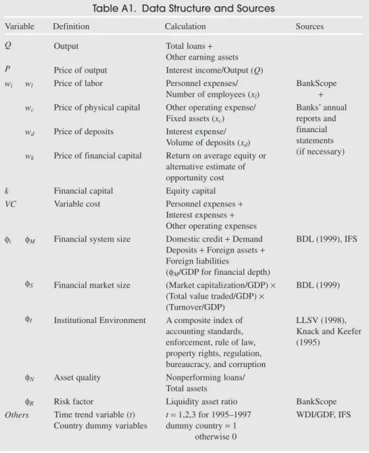
Tables A1 and A2 in the Appendix report, respectively, the data structure and sources and the descriptive statistics.
16Although these indicators include only banking variables, they should indirectly reflect also the size of some of the main infrastructural components underpinning the financial system (e.g., payment and clearing systems, legal/regulatory/supervisory systems, information systems and services, liquidity facili-ties and safety nets, etc.).
17A detailed classification of the sampled countries is reported in Bossone and Lee (2002). We had ini-tially considered including a fourth subgroup of three very small open economies, namely, Bermuda, Liechtenstein, and Monaco, whose FSis assumed to be less than US$1 billion. Because of the volatile estimates derived, we eventually decided to exclude these countries from our analysis in Section IV.
18The reason for combining three types of stock market development indicators is to obtain a more reliable and comprehensive measure, especially in some emerging countries.
IV. Empirical Results Existence of SSEs
The parametric measures of scale economies reveal the presence of significant scale economies associated with different indicators of financial system size (Table 1).20Interestingly, SSEs are not detected by the conventional measures,21 while they turn out to be greater than one and increasing when the adjustment fac-tors are incorporated in measurement.
20This evidence in support of SSEs is also confirmed by regressing the various measures of scale economies on different size indicators of financial system and markets and on a number of variables reflect-ing bank market structure, risk environment, and institutional characteristics. See Bossone and Lee (2002) for details.
21In a broad sense, εTCQcan be viewed as a sort of adjusted measure for εVCQ, but here it is regarded as a conventional measure in that no asset-quality adjustment was made.
Table 1. Scale Economies and Financial and Institutional Variables
Conventional Measure1 Quality-Adjusted Measures1
Financial and Institutional Variables2 εVCQ εTCQ εq
VCQ ε
q TCQ
Financial System Small (126) 1.04 0.99 0.92 0.89
Size3(FS) Medium (252) 0.93 0.97 0.97 1.02
Large (2,226) 0.87 0.98 1.04 1.18
Financial System Low (675) 0.95 0.98 0.98 1.02
Depth (FD*MS) High (1,950) 0.86 0.98 1.05 1.19
Financial Market Small (1,329) 0.92 0.98 1.01 1.08
Size (MS) Large (1,296) 0.85 0.97 1.04 1.20
Asset Quality (qa) Low4(879) 0.83 0.97 1.04 1.22
High (1,746) 0.91 0.98 1.02 1.10
Institutional Low5(378) 0.97 0.97 0.95 0.96
Environment (INST) High (2,247) 0.87 0.98 1.04 1.17 Corruption (CORP) High6(312) 0.98 0.97 0.95 0.95
Low (2,313) 0.87 0.98 1.04 1.17
Information Low (330) 0.98 0.98 0.95 0.96
Transparency (AS) High (2,295) 0.87 0.98 1.04 1.17 Market Concentration Low7(2,016) 0.87 0.98 1.04 1.18
(CN)8 High (609) 0.95 1.03 0.98 1.03
Notes: 1) The shaded area represents higher-scale economies for each classification of financial variables.
2) The figures in parentheses represent the number of observations. 3) In billions of U.S. dollars.
4) The lower asset quality means the higher NPL ratio. 5) Less than 6.0 (0 < INST< 10.0)
6) Less than 4.0 (0 < CORP< 6.0) 7) Less than 0.5 (0 < CN< 1.0)
8) All the parametric estimates are statistically different at the 5 percent significance level. Differences refer to comparisons of conventional vs. adjusted measures; small vs. large classes; and low vs. high classes.
This suggests that the SSEs in financial capitalization and risk management are relevant in bank production. In particular, Table 1 shows that scale economies change markedly in response to changes in bank asset quality and in the bank risk environment as proxied by indicators of information transparency, institutional strength, and corruption. The results suggest that reputation signaling for banks with sound assets can be more efficient than for risky banks, the reason being that low-risk banks may be able to signal added levels of low-risk protection with fewer additional resources than high-risk banks and save on risk-management costs, or even reduce their cost of funding, by signaling more financial strength. Higher cost efficiency due to better signaling can also explain why banks operating in a highly transparent environment can expand production with a less than proportional increase in the cost of nonfinancial and financial resources needed to manage risks, as compared to banks operating in more opaque environments. Finally, higher cost efficiency in risk management and financial capitalization is possible for systems with stronger insti-tutions and better governance.
Consistent with the importance of the factors relating to risk and informa-tion is the apparently counterintuitive finding that lower market concentrainforma-tion increases scale efficiency.22Where competition is stronger (which is typically the case in larger and more developed financial systems), investor risk sensitiv-ity is higher and signaling—as well as signal extraction—can be done more effi-ciently. As a result, scale economies associated with financial capitalization and risk management are larger than when competition is weaker, and banks do not need to invest as much in risk management and reputation signaling as they increase their output.
These results also raise issues relating to the relationship between banks and financial markets, discussed in Box 1.
The positive relationship between financial system size and scale efficiency in financial capitalization and risk management is illustrated quite clearly by Table 2, which reports the values of adjusted scale economies for subgroups of banks by bank scale and financial system size and shows that economies of scale increase with both bank scale and system size.
Two interesting observations from Table 2 are that small banks in large sys-tems are considerably more cost-efficient than small banks in small syssys-tems (1.06 and 0.93, respectively) and that, on the whole, bank scale does not make much of a difference within classes of financial system size.
Additional evidence in support of SSEs in production and risk management can be found by analyzing bank cost structures. From production theory, the elasticity of variable cost to output can be expressed as the ratio of marginal cost to average cost.23Using a hypothetical total cost function that incorporates the shadow cost 22Since a dominant domestic bank operating in a highly concentrated market has a lower demand for financial capital (see equation (5)), one should expect a positive relationship to hold in principle between market concentration and scale economies (as long as the marginal cost of financial capital, or the cost of signaling, is positiveas in Hughes and Mester, 1998).
Box 1. Banks and Financial Markets: Supplements or Complements?
Consistent with recent findings,24the results in Table 1 support the existence of
complemen-tarities between banks and financial market institutions. However, unlike previous studies and evidence, and in line with our SSE hypothesis, the results point to complementarities running from markets to banks. They show how bank efficiency benefits from developed financial markets in the face of the prediction from well-known studies whereby developed financial markets ultimately cause the banking sector to shrink.25
In fact, our results do not necessarily contradict that prediction. The informational externalities springing from efficient financial markets strengthen the competitiveness of those banks that are best equipped to benefit from better information use. In this case, only such banks are able to survive in an otherwise shrinking traditional banking business sector, while others are forced to exit the market. Furthermore, the presence of efficient financial markets allows banks to improve their risk-management capacity and, hence, their potential to expand their business into nonbanking financial areas, where demand for cross-sectional risk-sharing services is high and growing vis-à-vis the consolidating market of deposit and loan contracts.26
Accordingly, the development of financial markets dynamically induces banking to shift from activities that stand to lose from competition with financial market services to those that exploit complementarities with financial markets.
It must be noted, however, that while traditional banking activities tend to consolidate, they retain key functions—such as money creation (Bossone, 2001) and contingent liquidity provision to nonbank financial institutions (Corrigan, 2000)—that are essential to the function-ing and development of financial markets. These functions not only underpin fundamental complementarities running from banks to markets, but point to the fact that traditional banking business cannot be reduced beyond certain limits.
24Demirgüç-Kunt and Levine (1996, 2001) find evidence of strong complementarities between bank and capital-market financing in affecting economic growth. Evidence showing that banks supply capital markets with valuable information is reported by James (1987), Slovin, Sushka, and Hudson (1988), Lummer and McConnell (1989), and Biller, Flannery, and Garfinkel (1995).
25See for instance Jacklin (1987), Jacklin and Bhattacharya (1988), Diamond (1997), and Allen and Gale (1999, 2002).
26For the expansion of banks into the business of cross-sectional risk-sharing business, and their dis-intermediation from traditional activities, see Allen and Santomero (2001).
27The reason for using a shadow total cost function here is that it is difficult to obtain a quality-adjusted ACand MCdirectly with the underlying variable cost function. Note that the indirect measure of scale economies, derived from the ratio of AC/MCin the bottom line of Table 3 will be slightly different from that of other direct measures, due to rounding and aggregation errors of computation.
of financial capital, CT = CV + (−∂CV/∂k)k,27 we estimated the average-cost /
marginal-cost ratio for each subgroup of banks by bank scale and financial system size (Table 3). Note that ratio values larger (smaller) than 1 imply economies (dis-economies) of scale. It can be observed that both average and marginal costs decrease as the size of the banks and the financial system increases. Also, scale economies increase with the size of the financial system.
28Reductions in the quantity of labor inputs due to scale economies can be more than offset by the increase in the cost of labor inputs.
Table 2. Adjusted Scale Economies
by Size of Banks and Financial Systems Financial System Size (FS)
Bank Size (ta) Small Medium Large Total Small 0.93 (96)1, 2 0.99 (84) 1.06 (690) 1.04 (876)
Medium 0.91 (24) 0.98 (102) 1.04 (738) 1.03 (876)
Large 0.94 (6) 0.96 (66) 1.02 (798) 1.01 (873)
Total 0.92 (126) 0.97 (252) 1.04 (2,226) 1.03 (2,625)
Notes: 1) The figures in parentheses are the numbers of sample bank observations. 2) All are 1995–97 mean values for each subgroup.
SSEs in Production and Risk Management
With robust evidence supporting the existence of SSEs, it is now interesting to try to determine the quantitative relevance of the individual SSE channels discussed in Section II. A good starting point is the decomposition of the adjusted scale economies measure (Table 4). The following interesting features emerge from such decomposition. First, financial system size negatively affects bank production costs (component A), perhaps as a result of the disproportionate variations in labor costs observed across financial system sizes.28
Second, banks in large systems more than offset production diseconomies through cost savings generated by financial capitalization (in other words, addi-tional capital reduces variable costs), whereas this option is not available to banks in small systems (component B).
Third, changes in bank risk level generate larger cost increases in large systems than in small ones (component C). This is consistent with the findings discussed above concerning the relevance of the bank risk-environment factors: in larger sys-tems, with more efficient information provision and more signal-extraction capac-ity, investors are more reactive to changes in risks, value-maximizing banks allocate more resources to managing risks, and the banks’ cost of funding is more sensitive to changes in risk perceptions.
Fourth, in larger systems banks can offset such diseconomies by adding more capital (component D), suggesting that where information is provided and used more efficiently, signaling more financial strength allows banks to save on risk-management costs and possibly reduce their cost of funding. Once again, this option is not available to banks in small systems.
As discussed under Proposition 1, another source of evidence of SSEs is the presence of dynamic efficiency effects of financial system size on bank costs, due to changes in technology. We estimated such effects indirectly by including the time trend term (t) in our model specification, as a proxy for technical progress, and by
Table 3. Average and Marginal Total Cost
by Size of Banks and Financial Systems Financial System Size (FS)
Bank Size (ta) Small Medium Large Total Small 0.094 (0.091)1, 2 0.116 (0.108) 0.083 (0.075) 0.087 (0.080) Medium 0.097 (0.091) 0.081 (0.078) 0.079 (0.073) 0.079 (0.074) Large 0.070 (0.068) 0.073 (0.070) 0.068 (0.065) 0.068 (0.066) Total3 0.093 (0.090) 0.091 (0.086) 0.076 (0.071) 0.078 (0.073) [εTCQ=AC/MC] [1.03] [1.06] [1.08] [1.07]
Notes: 1) Marginal costs are reported in parentheses. 2) All are 1995–97 mean values for each subgroup.
3) 15 outlier observations for MC(negative or close to 0) are excluded in the calculation of average in the case of small and medium financial systems.
Table 4. Decomposition of Adjusted Scale Economies
by Financial System Size1
Sources
Financial System Size (FS)
Small 0.9626 0.0923 0.0067 0.0224 0.9249
Medium 1.0778 −0.0724 0.0450 −0.0226 0.9745
Large 1.1555 −0.1928 0.0628 −0.0613 1.0390
Notes: 1) All numbers are mean values during 1995–97 for each subgroup.
2) will not be exactly the same as 1/(A+B+C+D), due to averaging and rounding errors. εVCQ q εVCQq A B C D 2 1= + + + ( ) ∂ ∂ ∂ ∂ ( ) ln ln ln ln C k k q D V a ∂ ∂ ( ) ln ln C q C V a ∂ ∂ ∂ ∂ ( ) ln ln ln ln C k k Q B V ∂ ∂ ( ) ln ln C Q A V
measuring the impact of technical change on bank variable cost controlling for finan-cial system size. We derived parametric estimates of technical change over the vari-able cost function estimated for each class of financial system size. Differentiating the variable cost function with respect to tand taking it with the negative sign yield a measure of technical progress (Baltagi and Griffin, 1988):
(10) where εVCt> 0 implies a cost saving over time.
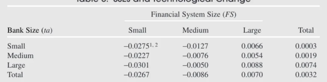
Table 5 compares the estimates of εVCt reported as yearly rates of variable
cost variation. Only banks operating in large financial systems show a decreasing rate of variable cost (0.7 percent annually). On the other hand, banks in medium-sized systems show an annual rate of increment (0.09 percent), and those in small systems have a much higher rate of cost increment (2.7 percent). Note that the
εVCt α β V t it i i C t Z = − ∂ ∂ = −
(
+∑
)
ln ln ,estimated cost function includes country-specific differences, so that the esti-mated technology-related SSE effects are not affected by the different levels of economic development.
Observing the parameter estimates for βitin equation (10),29it can be noticed
that the sign of the coefficient for deposits (d) and physical capital (c) and for the scale-related variables of output (Q), financial system (FS), and market size (MS) is negative. This implies that a larger bank operating at a large scale of deposits and loans within a large and deep financial system is expected to show quite a large cost savings over time. Table 5 confirms that the overall rate of cost saving is high-est in the large banks in large systems. On the other hand, the high-estimates for εVCtin
the small and medium systems are negative, indicating weak scale effects. The derived estimates can be interpreted as the rates of change in cost, over the sample period considered, made possible by technology development through the interaction of network externalities and scale economies. The findings support the hypothesis that the size of the financial system matters and suggest that small banks operating in large financial systems are financially more viable than small banks operating in small systems.
Proposition 2 predicates that SSEs are associated with large, deep, and efficient financial markets. Access to larger markets reduces bank costs by providing banks with more efficient instruments of risk management and reputation signaling, which enable them to economize on the financial capital required by higher production. This is supported by the estimated parameters of the endogenous demand equation for financial capital (equation (5)), which shows that the demand for financial capi-tal increases with output and nonperforming loans, while it decreases with the size of the capital markets (Table 6).
Since each parameter of equation (5) represents an elasticity coefficient of the demand for capital, we were able to gauge how much additional financial capital is required with respect to changes in each of the components of the financial capital demand function. We defined the total elasticity of financial capital (εk) for each
29Maximum likelihood estimation results yield εVCt= −(0.0355 +0.0117 ln w
l−0.0092 ln wd−0.0025
ln wc+0.0013 ln k+0.0009 ln qa−0.0048 ln Q−0.0065 ln FS−0.0002 ln MS+0.0234 t).
Table 5. SSEs and Technological Change
Financial System Size (FS)
Bank Size (ta) Small Medium Large Total
Small −0.02751, 2 −0.0127 0.0066 0.0003
Medium −0.0227 −0.0076 0.0054 0.0019
Large −0.0301 −0.0050 0.0088 0.0074
Total −0.0267 −0.0086 0.0070 0.0032
Notes: 1) The figures represent rates of technical progress. Positive (negative) values indicate annual rates of cost diminution (increment) during the sample period.
class of financial system size, averaged over country (j) and under constant macro financial factors, as
(11)
where the elasticity of financial capital with respect to output is broken down by financial system size, as indicated by the superscript s(indicating small, medium,
and largesystem size). Elasticity εSkmeasures the total economies in capitalization
in each subgroup of banks in the different classes of financial system size.30 According to the results reported in Table 6, where the coefficients (column 1) are allowed to vary across different financial systems, the overall sum of the par-tial elasticities is the highest for banks in small systems (1.402).
The results show that, as output increases, banks operating in medium and large financial systems require a less than proportionate increase in financial cap-ital than those operating in small systems. This implies that, as the financial sys-tem becomes larger and deeper, banks need relatively less financial capital to manage risks and to signal their strength to the market as they expand production. Note, in line with Proposition 2, the significant SSE effect of financial market depth and efficiency (MS) once the absolutesize of the financial system (FS) is controlled for. This suggests that, for any given size of the financial system, more
εk s
( )
˜ εkQ s ε ε ε ε ε ε k S j j S n a kQ s kFS kMS kq kCN n k Q k FS k MS k q k CN = ∂ ∂ + ∂∂ + ∂∂ + ∂∂ + ∂∂ = +[ + + + ] ∈∑
1 ln ln ln ln ln ln ln ln ln ln ˜ ,30This coefficient is equivalent to the Hughes and Mester (1998) measure of economies capitalization (ELSTK), whose reported value was 0.7153 with asset quality adjustment for the U.S. banking system.
Table 6. Economies of Capitalization and Financial System Size1, 2
Financial ε∼skQ3 εkFS εkMS εkq εkCN εSk System Size (FS) (1) (2.1) (2.2) (2.3) (2.4) (1) +(2) Small 1.881*** 1.402*** (10.81) (2.95) Medium4 1.541*** 0.217 −0.169*** 0.473*** −1.001*** 1.062** (0.96) (14.95) (2.57) (8.03) (3.22) (2.45) Large 1.526*** 1.047** (19.85) (2.55) Total4 1.660*** 1.181*** (17.45) (2.73)
Notes: 1) The figures in parentheses beneath the estimates are t-statistics.
2) *, **, *** indicate significance levels of 10, 5, and 1 percent, respectively.
3) ε∼skQis the average of parameter estimates within the same class of system size countries.
4) Here, three small open economies as a fourth subgroup (Bermuda, Liechtenstein, and Monaco) and two medium countries showing negative estimates (Argentina and Chile) were excluded.
efficient market infrastructures allow banks to use financial capital more effi-ciently (all else being equal).
The existence of SSEs in financial capitalization can be detected also by observ-ing the degree of utilization of financial capital by banks across different classes of financial system size. As assumed in Proposition 2, banks in small systems should systematically hold relatively larger stocks of financial capital than banks in large systems (all else being equal).
Before exploring the degree of financial capital utilization, we first need to get an equilibrium market rental price of capital (wk) that can be proxied easily. In
general, the most practical proxy readily available is the return on average equity (ROAE). Table 7 compares average ROAEs directly obtained from the BankScope database for each subgroup of different classes of bank scale and financial system size.
The overall sample average ROAEis 11 percent.31The ROAEsfor the small and medium financial systems (15 and 16 percent, respectively) are considerably higher than for large systems (10 percent). Among the different classes of bank size in terms of assets, small banks yield the highest ROAE(13 percent), followed by medium banks (11 percent), and by large banks (8 percent). However, since the ROAE may not be suited for our assumed single-product cost function, we used an alternative measure of wk, defined as (total revenue minus variable
cost)/equity capital). Such a measure is more consistent with the single-product cost function associated with the bank’s primary activity of lending.32 Table 7 reports in the parentheses beneath the ROAEsthe values of wk, calculated by size
of banks and financial systems. The average value for wkover total sample
obser-31Hughes and others (2001) performed a check for over- or underutilization of financial capital by assuming wkto be around 0.14 ∼0.18.
32The reported values of ROAEreflect the final result of all kinds of banking activities, including non-interest operating income (fees, commissions, etc.), as well as extraordinary income. Since our cross-sectional study was limited by data availability, we assumed a single-product (loans) cost function, instead of multiproduct cost function, allowing us to focus on the primary banking activities of lending and deposit. Consequently, our model specification requires that we use an adjusted measure of market rental price of equity capital (wk), rather than the unadjusted ROAE.
Table 7. Opportunity Cost of Financial Capital
by Size of Banks and Financial Systems1
Financial System Size (FS)
Bank Size (ta) Small Medium Large Total Small 0.15 (0.02)2 0.18 (0.12) 0.12 (0.08) 0.13 (0.07) Medium 0.19 (0.05) 0.16 (0.14) 0.10 (0.09) 0.11 (0.10) Large 0.12 (0.11) 0.16 (0.05) 0.08 (0.07) 0.08 (0.07) Total 0.15 (0.03) 0.16 (0.11) 0.10 (0.08) 0.11 (0.08)
Notes: 1) All numbers are 1995–97 mean values of ROAEand wkfor each subgroup.
vations is 0.08, which is lower by 0.03 point than the ROAE(0.11). Interestingly, the average value of wkin medium-sized banks (0.10) and medium-sized systems
(0.11) is the highest of their respective classes. It can be observed that, on the whole, wk appears to be consistently smaller than the ROAE across different
classes of bank and system size.33
In order to investigate whether the level of financial capital changes system-atically with financial system size, we also need a shadow measure of the price of capital (w*k), which can be analytically derived from the restricted variable cost
function (i.e., ∂CV/∂k), thus enabling us to compare whether wkis greater than
w*k. Table 8 reports the average value of w*k, obtained by calculating the realized value of (∂CV/∂k).
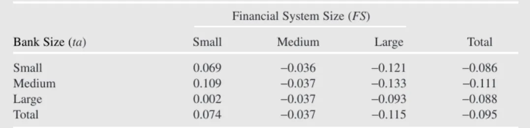
As shown in the table, the marginal (or shadow) cost of financial capital is neg-ative both in medium (−0.037) and large (−0.115) systems, while it is positive in small systems (0.074). If we interpret the marginal cost of financial capital as rep-resenting the cost incurred by banks to signal their strength to the market (Hughes and Mester, 1998), our results seem to suggest that there are system-dependent scale efficiency effects in the cost of financial capital. As argued earlier, this may be due to the higher efficiency of information provision and signaling that character-ize larger systems vis-à-vis smaller ones.
Finally, comparing the equilibrium price (wk) with the marginal (shadow) cost of
financial capital (w*k) in Table 9 gives an indication of the degree of utilization of
financial capital by banks: if the marginal cost exceeds (is lower than) the equilib-rium price, financial capital is being over- (under-) utilized, while their equality indi-cates optimal utilization.
Notice from Table 8 that the marginal cost of financial capital observed over the whole sample is negative (−0.095), implying that financial capital is an effi-cient risk-management instrument and signaling device for banks: a higher level of capital indicates a lower risk and reduces the equilibrium market price of
33A possible explanation for the systematically lower values is that most of the sample banks largely operate in non-interest income activity areas. Since we assume a single-product function (see previous footnote), the associated total (interest) income is smaller than the income associated with a multiproduct function.
Table 8. Shadow Cost of Financial Capital (∂CV/ ∂k)
by Size of Banks and Financial Systems1
Financial System Size (FS)
Bank Size (ta) Small Medium Large Total
Small 0.069 −0.036 −0.121 −0.086
Medium 0.109 −0.037 −0.133 −0.111
Large 0.002 −0.037 −0.093 −0.088
Total 0.074 −0.037 −0.115 −0.095
capital, signifying a lower risk. However, this does not hold for banks in small financial systems.
The observed utilization of financial capital, estimated by size of banks and financial systems ( Table 9), suggests that banks overutilize capital in small and medium-sized systems, while they underutilize it in large systems. Only the large banks in the large systems operate close to an optimal capital range (the overall mean value of (wk+ ∂CV/∂k) is −0.035).
V. Conclusion
Based on the general assumption that finance involves increasing returns to scale of various sorts, this study has formulated and tested empirically the systemic scale economies (SSEs) hypothesis, whereby the production efficiency of financial intermediation increases with the size of the system where it takes place. Using a large cross-country and time-series banking data panel, the study has shown that intermediaries operating in systems with large markets and infrastructures have lower production costs and lower costs of risk absorption and reputation signaling than intermediaries operating in small systems. The study has explored different channels through which the SSEs work their effects on intermediaries and has derived statistically significant estimates of such effects. In particular, the results show that
• SSEs can be detected when risk is endogenized in bank production decisions and banks are modeled as value-maximizing agents.
• Larger, deeper, and more efficient financial systems enable banks to save on the resources needed to manage the higher risks associated with larger production. • Small banks in large systems are more cost-efficient than small banks in small
systems.
• The cost-efficiency effects of technological changes are more rapid for banks operating in larger systems.
• Banks in small (large) systems tend to over- (under-) utilize financial capital, while large banks in large systems operate at an approximately optimal capi-tal level.
Table 9. Utilization of Financial Capital by
Size of Banks and Financial Systems Financial System Size (FS)
Bank Size (ta) Small Medium Large Total
Small 0.0851, 2 0.081 −0.043 −0.014
Medium 0.157 0.105 −0.038 −0.015
Large 0.116 0.015 −0.024 −0.021
Total 0.100 0.074 −0.035 −0.013
Notes: 1) The figures are obtained from (wk+ ∂CV/ ∂k). Positive (negative) values indicate
over-(under-) utilization.
More generally, one may conclude that the minimum size for a bank to be mar-ket viable decreases with the size of the financial system where it operates. As a consequence, stronger competition (or lower market concentration) can fully trans-late into higher scale efficiency for individual banks only in system size above a certain threshold level.
The results have also shown that information transparency, institutional devel-opment (that is, better financial infrastructure), and good governance allow inter-mediaries to achieve considerable scale efficiency gains.
The evidence produced by this study has shown that the financial intermediaries in small systems operate at a comparative disadvantage with respect to those oper-ating in larger systems. The evidence supports the intuition underpinning the work by Bossone, Honohan, and Long (2001) and strengthens the case for their policy recommendations.
APPENDIX
Table A1. Data Structure and Sources
Variable Definition Calculation Sources
Q P wi k VC φi Others wl wc wd wk φM φS φI φN φR Output Price of output Price of labor
Price of physical capital Price of deposits Price of financial capital
Financial capital Variable cost
Financial system size
Financial market size
Institutional Environment
Asset quality Risk factor
Time trend variable (t) Country dummy variables
Total loans + Other earning assets Interest income/Output (Q) Personnel expenses/ Number of employees (xl)
Other operating expense/ Fixed assets (xc)
Interest expense/ Volume of deposits (xd)
Return on average equity or alternative estimate of opportunity cost Equity capital Personnel expenses + Interest expenses + Other operating expenses Domestic credit +Demand Deposits +Foreign assets + Foreign liabilities
(φM/GDP for financial depth) (Market capitalization/GDP) × (Total value traded/GDP) × (Turnover/GDP)
A composite index of accounting standards, enforcement, rule of law, property rights, regulation, bureaucracy, and corruption Nonperforming loans/ Total assets
Liquidity asset ratio t=1,2,3 for 1995–1997 dummy country =1 otherwise 0 BankScope + Banks’ annual reports and financial statements (if necessary) BDL (1999), IFS BDL (1999) LLSV (1998), Knack and Keefer (1995)
BankScope WDI/GDF, IFS
Table A2. Descriptive Statistics
Variable Descriptions Average1 Min Max
Micro Banking Variables
Q Aggregate output2 19.4 0.4 629.4
xl Total number of employees 4554.4 7.7 87933.3
xd Total deposits2 15.0 0.1 454.4
xc Fixed assets2 0.3 0.0 7.2
K Financial (equity) capital2 1.0 0.0 24.0
R Liquidity asset ratio (percent) 24.4 0.0 667.7
q Nonperforming loan ratio (percent) 4.0 0.0 81.8
P Price of output3 0.1 0.0 0.4
wl Price of labor3 52.1 1.8 227.0
wd Price of deposits3 0.1 0.0 5.8
wc Price of physical capital3 1.0 0.0 11.1
wk Price of financial capital (percent) 10.8 −111.5 73.7
VC Variable cost2 12.3 0.0 38.0
Macro Financial Variables
MS Financial market size 36.5 0.0 1326.8
(Costa Rica) (Taiwan)
FS Financial system size2 967.5 2.4 20467.2
(Bermuda) (Japan)
M22 233.7 1.3 5261.4
(Estonia) (United States)
INST Institutional Environment 6.18 0.24 10.0
(Bangladesh) (Netherlands)
AS Accounting standards 58.3 24.0 83.0
(Bangladesh) (Sweden)
CORP Corruption 4.11 0.61 6.0
(Bangladesh) (10 countries)4
CN Banking market concentration 0.625 0.186 1.0
ratio5 (United States) (5 countries)6
Notes: 1) All price-related figures are inflation-adjusted and expressed in U.S. dollars. The means of micro banking variables are calculated for 875 banks over 1995–1997. 2) In U.S. billions of dollars.
3) In U.S. thousands of dollars.
4) Sweden, Iceland, Luxembourg, Finland, Norway, Switzerland, Canada, Denmark, New Zealand, Netherlands.
5) Share of the assets of three largest banks in total banking assets. 6) Algeria, Bermuda, Ethiopia, Liechtenstein, and Monaco.