How Java Programs Interact with Virtual Machines
at the Microarchitectural Level
Lieven Eeckhout
Andy Georges
Koen De Bosschere
Department of Electronics and Information Systems (ELIS), Ghent University St.-Pietersnieuwstraat 41, B-9000 Gent, Belgium
{leeckhou,ageorges,kdb}@elis.UGent.be
ABSTRACT
Java workloads are becoming increasingly prominent on var-ious platforms ranging from embedded systems, over general-purpose computers to high-end servers. Understanding the implications of all the aspects involved when running Java workloads, is thus extremely important during the design of a system that will run such workloads. In other words, understanding the interaction between the Java application, its input and the virtual machine it runs on, is key to a suc-cesful design. The goal of this paper is to study this complex interaction at the microarchitectural level, e.g., by analyz-ing the branch behavior, the cache behavior, etc. This is done by measuring a large number of performance charac-teristics using performance counters on an AMD K7 Duron microprocessor. These performance characteristics are mea-sured for seven virtual machine configurations, and a collec-tion of Java benchmarks with corresponding inputs coming from the SPECjvm98 benchmark suite, the SPECjbb2000 benchmark suite, the Java Grande Forum benchmark suite and an open-source raytracer, called Raja with 19 scene de-scriptions. This large amount of data is further analyzed using statistical data analysis techniques, namely principal components analysis and cluster analysis. These techniques provide useful insights in an understandable way.
From our experiments, we conclude that (i) the behavior observed at the microarchitectural level is primarily deter-mined by the virtual machine for small input sets, e.g., the
SPECjvm98s1input set; (ii) the behavior can be quite
dif-ferent for various input sets, e.g., short-running versus long-running benchmarks; (iii) for long-long-running benchmarks with few hot spots, the behavior can be primarily determined by the Java program and not the virtual machine, i.e., all the virtual machines optimize the hot spots to similarly behav-ing native code; (iv) in general, the behavior of a Java appli-cation running on one virtual machine can be significantly different from running on another virtual machine. These conclusions warn researchers working on Java workloads to be careful when using a limited number of Java benchmarks
Permission to make digital or hard copies of all or part of this work for personal or classroom use is granted without fee provided that copies are not made or distributed for profit or commercial advantage and that copies bear this notice and the full citation on the first page. To copy otherwise, to republish, to post on servers or to redistribute to lists, requires prior specific permission and/or a fee.
OOPSLA’03, October 26–30, 2003, Anaheim, California, USA.
Copyright 2003 ACM 1-58113-712-5/03/0010 ...$5.00.
or virtual machines since this might lead to biased conclu-sions.
Categories and Subject Descriptors
C.4 [Performance of Systems]: design studies,
measure-ment techniques, performance attributes
General Terms
Measurement, Performance, Experimentation
Keywords
workload characterization, performance analysis, statistical data analysis, Java workloads, virtual machine technology
1.
INTRODUCTION
In the last few years, the Java programming language is taking up a more prominent role in the software field. From high-end application servers, to webservers, to desktop ap-plications and finally to small apap-plications on portable or embedded devices, Java applications are used in virtually every area of the computing sector. Not only Java applica-tions are abundant, the advent of the language also intro-duced various virtual machines capable of executing these applications, each with their own merits and drawbacks.
We can distinguish three important aspects that possibly have a large impact on the overall behavior of a Java work-load: the virtual machine executing the Java bytecode, the Java application itself and the input to the Java application. For example, concerning the virtual machine, the choice of interpretation versus Just-in-Time (JIT) compilation is a very important one. Also, the mechanism implemented for supporting Java threads as well as for supporting garbage collection can have a large impact on the overall perfor-mance. Secondly, the nature of the Java application itself can have a large impact on the behavior observed by the mi-croprocessor. For example, we can expect a database appli-cation to behave differently from a game appliappli-cation. Third, the input of the Java application can have a significant im-pact on the behavior of a Java workload. For example, a large input can cause a large number of objects being cre-ated during the execution of the Java application stressing the memory subsystem. Each of these three aspects can thus have a large impact on the behavior as observed at the microarchitectural level (in terms of branch behavior, cache behavior, instruction-level parallelism, etc.). This close
teraction between virtual machine, Java application and in-put is hard to understand due to the complex behavior of Java workloads. Therefore, we need techniques to get better insight in this interaction.
The main question we want to address in this paper is thus the following: how much of the behavior as observed at the microprocessor level is due to the virtual machine, the Java application, and the input to the application? For ex-ample, most virtual machines currently employ a JIT com-pilation/optimization strategy. But how big is the impact of the actual implementation of the JIT engine on the observed behavior? I.e., do virtual machines implementing more or less the same strategy behave similarly? Secondly, how large is the impact of the Java application? Is the behavior of a Java workload primarily determined by the Java application or by the virtual machine? And what is the impact of the input to the Java application?
In the last few years, valuable research has been done on characterizing Java workloads to get better insight in its be-havior, see also the related work section at the end of the paper. Previous work typically considered only one or two virtual machines in their methodology as well as only one benchmark suite, mostly SPECjvm98. In addition, some
studies use a small input set, e.g., s1 for SPECjvm98, to
limit the simulation time in their study. As such, we can raise the following questions in relation to previous work. Is such a methodology reliable for Java workloads? What happens if the behavior of a Java workload is highly de-pendent on the chosen virtual machine? Can we translate conclusions made for one virtual machine to another vir-tual machine? Also, is SPECjvm98 representative for other Java applications? I.e., are the conclusions taken based on SPECjvm98 valid for other Java programs? And is using a
small input, e.g., SPECjvm98s1, yielding a short-running
Java workload representative for a large input, e.g., s100,
yielding a long-running Java workload?
To answer these questions, we use the following method-ology. First, we measure workload characteristics through performance counters while running the Java workloads on real hardware, in our case an AMD K7 Duron microproces-sor. This is done for a large number of virtual machine con-figurations (7 in total) as well as for a large number of Java applications with corresponding inputs. The benchmarks and their inputs are taken from the SPECjvm98 suite, the SPECjbb2000 suite and the Java Grande Forum suite. In addition, we also include a raytracer with 19 scene descrip-tions. Second, a statistical analysis is done on these data using principal components analysis (PCA) [17]. PCA is a multivariate statistical data reduction technique capable of increasing the understandability of the large amounts of data. The basic idea of this statistical analysis is as follows.
Java workloads could be displayed in an-dimensional space,
withnthe number of performance characteristics measured
in the previous step. However, the dimension of this spacen
is too large to be understandable, in our studyn= 34. PCA
reduces this high dimensional space to a lower dimensional and uncorrelated space, typically 4-D in our experiments without loosing important information. This increases the understandability for two reasons: (i) its lower dimension and (ii) there is no correlation between the axes in this space. In the third step of our methodology, we display the Java workloads in this lower dimensional space obtained af-ter PCA. In addition, we further analyze this reduced Java
workload space through cluster analysis (CA) [17]. This methodology will allow us to address the questions raised in this paper. Indeed, Java workloads that are far away from each other in this space show dissimilar behavior whereas Java workloads close to each other show similar behavior. As such, if Java workloads are clustered per virtual machine, i.e., all the Java applications running on one particular vir-tual machine are close to each other, we can conclude that the overall behavior is primarily determined by the virtual machine and not the Java application. Likewise, if Java workloads are clustered per Java application, we conclude that the Java application has the largest impact and not the virtual machine. Also, if a Java program running differ-ent inputs results in clustered data points, we can conclude that the input has a small impact on the overall behavior.
Answering the questions raised in this paper is of inter-est for various research domains. First, Java application developers can get insight in the behavior of the code they are developing and how their code interacts with the virtual machine and its input. For example, if the overall behavior is primarily influenced by the virtual machine and not the Java application, application developers will pay less atten-tion to the performance of their code but will focus more on its reusability or reliability. Second, virtual machine de-velopers will get better insight in what sense the behavior of a Java workload is influenced by the virtual machine im-plementation and more in particular, how Java programs interact with their virtual machine design. Using this in-formation, virtual machine developers might design better VMs. Third, microprocessor designers can get insight in how Java workloads behave and how their microprocessors should be designed to address specific issues posed by Java workloads. Also, for microprocessor designers who heavily rely on time-consuming simulations, it is extremely useful to know whether small inputs result in similar behavior as large inputs and can thus be used to reduce the total simulation time without compromising the accuracy of their simulation runs [13].
This paper is organized as follows. In the next section, we present the experimental setup of this paper. We distin-guish four components in our setup: (i) the Java workloads, consisting of the virtual machine, the Java benchmarks and if available, various inputs for each of these benchmarks; (ii) the hardware platform, namely the AMD K7 Duron micro-processor; (iii) the measurement technique, i.e., the use of on-chip performance counters; and (iv) the workload char-acteristics we use in our methodology. In section 3, we dis-cuss the statistical data analysis techniques, namely princi-pal components analysis (PCA) and cluster analysis (CA). In section 4 we present the results we obtain through our analysis and extensively discuss the conclusions that can be taken from these. Section 5 discusses related work on char-acterizing Java workloads. Finally, we conclude in section 6.
2.
EXPERIMENTAL SETUP
2.1
Java workloads
This section discusses the virtual machines and the Java applications that are used in this study.
2.1.1
Virtual machines
In our study, we have used seven virtual machine config-urations which are tabulated in Table 1: SUN JRE 1.4.1,
Blackdown JRE 1.4.1 Beta, IBM JRE 1.4.1, JikesRVM, JRockit and Kaffe.
Both the SUN JRE 1.4.1 and the Blackdown JRE 1.4.1 Beta virtual machines are based on the same SUN HotSpot virtual machine core [26]. HotSpot uses a mixed scheme of interpretation, Just-in-Time (JIT) compilation and mization to execute Java applications. The degree of opti-mization can be specified by choosing either client mode or server mode. In client mode, the virtual machine performs fewer runtime optimizations resulting in a limited applica-tion startup time and a reduced memory footprint. In server mode, the virtual machine performs classic code optimiza-tions as well as optimizaoptimiza-tions that are more specific to Java, such as null-check and range-check elimination. It is also interesting to note that HotSpot maps Java threads to na-tive OS threads. The garbage collector uses a fully accurate, generational copying scheme. New objects are allocated in the ‘nursery’ and moved to the ‘old object’ space when the ‘nursery’ is collected. Objects in the ‘old object’ space are reclaimed by a mark and sweep compacting strategy.
BEA Weblogic’s JRockit [6] is a virtual machine that is targeted at server-side Java. JRockit compiles methods upon their first invocation. At runtime, statistics are gath-ered and hot methods are scheduled for optimization. The optimized code replaces the old code while the virtual ma-chine keeps running. This way, an adaptive optimization scheme is realized. JRockit uses a mixed threading scheme,
called ThinThread, in whichnJava threads are multiplexed
onmnative threads. The virtual machine comes with four
possible garbage collection strategies. We have used the gen-erational copying version in our experiments, which is the default for heap sizes less than 128MiB.
Jikes [2, 3] is a Research Virtual Machine
(RVM)—pre-viously known as Jalape˜no—that is targeted at server-side
Java applications. Jikes is written entirely in Java and uses compilation throughout the entire execution (no interpre-tation). It is possible to configure the JikesRVM in differ-ent compiling modes: baseline compiler, optimizing compiler and adaptive compiler. We have used the baseline and adap-tive modes in our experiments. The threading system
multi-plexesnJava threads tomnative threads. There is a range
of garbage collection strategies available for this virtual ma-chine. Among them are copying, mark-and-sweep and gen-erational collectors as well as combinations of these strate-gies. We have used the non-generational copying scheme (SemiSpace).
Kaffe1
is an open source virtual machine. We have used version 1.0.7 in our experiments. Kaffe uses interpretation as well as JIT compilation. In addition, native threads can be used.
The IBM JRE 1.4.02
[25] also uses a mixed strategy by employing IBM’s JIT compiler as well as IBM’s Mixed Mode Interpreter (MMI).
Note that the choice of the garbage collector is not con-sistent over the virtual machine configurations. We have chosen the default garbage collector for each virtual ma-chine. This leads to different garbage collector mechanisms for different virtual machines as can be seen from Table 1. In section 4.4, we will evaluate the impact of the garbage collector on overall workload behavior. This evaluation will
1
http://www.kaffe.org
2
http://www.ibm.com
show that the choice of the garbage collector has a minor impact on the results of this paper and does not change the overall conclusions.
2.1.2
Java applications and their inputs
There are numerous Java applications available both in the public and the commercial domain. However, most of these are (highly) interactive. Using such applications for our purposes is unsuitable since the measurements would not be reproducable. As such, we used non-interactive Java programs with command line inputs. The applications we have used are taken from several sources, see also Table 2: SPECjvm98, SPECjbb2000, the Java Grande Forum suite, and Raja.
SPECjvm983
is a client-side Java benchmark suite consist-ing of seven benchmarks. For each of these, SPECjvm98 pro-vides three inputs: s1,s10ands100. Contradictory to what the input set names suggest, the size of the input set does not increase linearly. For some benchmarks, a larger input indeed increases the problem size. For other benchmarks, a larger input executes a smaller input multiple times. In the evaluation section, we will discuss the impact of the var-ious input sets on the behavior of the Java programs and their virtual machines. SPECjvm98 was designed to eval-uate combined hardware (CPU, caches, memory, etc.) and software aspects (virtual machine, kernel activity, etc.) of a Java environment. However, they do not include graphics, networking or AWT (window management).
SPECjbb2000 (Java Business Benchmark)4
is a server-side benchmark suite focussing on the middle-tier, the busi-ness logic, of a three-tier system. We have run the SPEC-jbb2000 benchmark with different numbers of warehouses: 2, 4 and 8 warehouses.
The Java Grande Forum (JGF) benchmark suite5
[9] is intended to study the performance of Java in the context
of so-called Grande applications, i.e., applications
requir-ing large amounts of memory, bandwidth and/or processrequir-ing power. Examples include computational science and engi-neering codes, large scale database applications as well as business and financial models. For this paper, we have cho-sen four large scale applications from the sequential suite which are suitable for uniprocessor performance evaluation. For each of these benchmarks, we have used the two avail-able problem sizes, small and large.
Raja6
is a raytracer in Java. We included this raytracer in our analysis since its distribution comes with 19 scene descriptions. As such we will be able to quantify the impact of the input on the behavior of the raytracer. Unfortunately, we were unable to execute this benchmark on the Jikes and Kaffe virtual machines.
We ran all the benchmarks with a standard 64MiB virtual machine heap size. For SPECjbb2000, we used a heap size of 256 MiB.
2.2
Hardware used
We have done all our experiments on a x86-compatible platform, namely a 1GHz AMD Duron (model 7). The mi-croarchitecture of the AMD Duron is identical to the AMD Athlon’s microarchitecture except for the reduced size of the
3 http://www.spec.org/jvm98 4 http://www.spec.org/jbb2000 5 http://www.javagrande.org 6 http://raja.sourceforge.net
Virtual machine Configuration used
SUN JRE 1.4.1 HotSpot client, generational non-incremental garbage collection
Blackdown JRE 1.4.1 HotSpot client, generational non-incremental garbage collection
JikesRVM base baseline compiler with copying garbage collection
JikesRVM adpt adaptive compiler with copying garbage collection
JRockit adaptive optimizing compiler, generational copying collector
Kaffe interpretation and JIT compilation, non-generational garbage collection
IBM JRE 1.4.1 interpretation and JIT compilation
Table 1: The virtual machine configurations we have used to perform our measurements.
SPECjvm98
201 compress A compression program, using a LZW method ported from 129.compress in the SPECCPU95 suite. Unlike 129.compress, it processes real data from several files. The various inputs are obtained by performing a different number of iterations through various input files. It requires a heap size of 20MiB and allocates 334MiB of objects.
202 jess An expert shell system, adapted from the CLIPS system. The various inputs consist of a set of puzzles to be solved, with varying degrees of difficulty. The benchmark requires a heap size of 2MiB while allocating 748MiB of objects. 209 db The benchmark performs a set of database requests on a memory resident database of 1MiB. The various inputs are obtained by varying the number of requests to the database. It requires a heap size of 16MiB and allocates 224MiB of objects.
213 javac This is the JDK 1.0.2 source code compiler. The various inputs are obtained by making multiple copies of the same input files. It requires a heap size of 12MiB, and allocates 518MiB of objects.
222 mpegaudio A commercial application decompressing MPEG Layer-3 audio files. The input consists of about 4MiB of audio data. The number of objects that are allocated is negligible.
227 mtrt A raytracer using two threads to render a scene. The various inputs are determined by the problem size. The benchmark requires a heap size of 16MiB and allocates 355MiB of objects.
228 jack An early version of JavaCC which is a Java parser generator. The various inputs make several passes through the same data. Execution requires a heap size of 2MiB while 481MiB of objects are allocated.
SPECjbb2000 A three-tier transaction system, where the user interaction is simulated by random input selection and the third tier, the database, is represented by a set of binary trees. The benchmark focuses on the business logic found in the middle tier. It is loosely based on the IBM pBOB benchmark [5]. About 256MiB of heap space is required to run the benchmark.
Java Grande Forum
search A program solving a connect-4 game, using an alpha-beta pruning technique. The problem size is determined by the starting position from which the game is solved. The heap size should be at least 6MiB for both inputs.
euler Solution for a set of time-dependent Euler equations modeling a channel with a bumped wall, using a fourth order Runge-Kutta scheme. The model is evaluated for 200 timesteps. The problem size is determined by the size of the mesh on which the solution is computed. The heap size that is required is 8MiB for the small input and 15MiB for the large input.
moldyn Evaluation of an N-body model for particles interacting under a Lennard-Jones potential in a cubic space. The problem size is determined by the number of particles. Both inputs need a heap size of 1 MiB.
raytracer A raytracer rendering a scene containing 64 spheres. The problem size is determined by the resolution of the rendered image. Both inputs require a heap size of 1 MiB.
Raja A Raytracer. We used the latest 0.4.0-pre4 version. Input variation is ob-tained by using a set of 19 scene descriptions.
component subcomponent description
memory hierarchy L1 I-cache 64KB two-way set-associative, 64-byte lines, LRU replacement
with next line prefetching
L1 D-cache 64KB two-way set-associative, 8 banks with 8-byte lines, LRU
write-allocate, write-back, two access ports 64 bits each
L2 cache 64KB two-way set-associative, unified, on-chip, exclusive
L1 I-TLB 24 entries, fully associative
L2 I-TLB 256 entries, four-way set-associative
L1 D-TLB 32 entries, fully associative
L2 D-TLB 256 entries, four-way set-associative
branch prediction BTB branch target buffer, two-way set-associative, 2048 entries
RAS return address stack, 12 entries
taken/not-taken gshare 2048-entry branch predictor with 2-bit counters
system design bus 200MHz, 1.6GiB per second
pipeline stages integer 10 cycles
floating-point 15 cycles
integer pipeline pipeline 1 integer execution unit and address generation unit
also allows integer multiply
pipeline 2 integer execution unit and address generation unit
pipeline 3 idem
floating-point pipeline pipeline 1 3DNow! add, MMX ALU/shifter and floating-point add
pipleine 2 3DNow!/MMX multiply/reciproce, MMX ALU and
floating-point multiply/divide/square root
pipeline 3 floating-point constant loads and stores
Table 3: The AMD K7 Duron microprocessor summary.
L2 cache (64KB instead of 256KB). As such, the Duron as well as the Athlon belong to the same AMD K7 proces-sor family [1, 12]. For more details on the AMD Duron that is used in this study we refer to Table 3. The AMD K7 is a superscalar microprocessor implementing the IA-32 instruction set architecture (ISA). It has a pipelined mi-croarchitecture in which up to three x86 instructions can be fetched. These instructions are fetched from a large prede-coded 64KB L1 instruction cache (I-cache). For dealing with the branches in the instruction stream, branch prediction is done using a global history (gshare) based taken/not-taken branch predictor, a branch target buffer (BTB) and a return address stack (RAS). Once fetched, each (variable-length) x86 instruction is decoded into a number of simpler (and fixed-length) macro-ops. Up to three x86 instructions can be translated per cycle.
These macro-ops are then passed to the next stage in the pipeline, the instruction control unit (ICU) which ba-sically consists of a 72-entry reorder buffer. From this re-order buffer, macro-ops are scheduled into an 18-entry in-teger scheduler and a 36-entry floating-point scheduler for integer and floating-point operations, respectively. The 18-entry integer scheduler is organized as a collection of three 6-entry deep reservation stations, each reservation station serving an integer execution unit and an address generation unit. The 36-entry point scheduler (FPU: floating-point unit) serves three floating-floating-point pipelines executing x87, MMX and 3DNow! operations. In the schedulers, the macro-ops are broken down to ops which can execute out-of-order. Next to these schedulers, the AMD K7 microarchi-tecture also has a 44-entry load-store unit. The load-store unit consists of two queues, a 12-entry queue for L1 D-cache load and store accesses and a 32-entry queue for L2 cache and memory load and store accesses—requests that missed
in the L1 D-cache. The L1 D-cache is organized as an eight-bank cache having two 64-bit access ports.
Another interesting aspect of the AMD K7 microarchi-tecture is the fact that the L2 unified cache is an exclusive cache. This means that cache blocks that were previously held by the L1 caches but had to be evicted from L1, are held in L2. If the newer cache block that is to be stored in L1 previously resided in L2, that cache block will be evicted from L2 to make room for the L1 block, i.e., a swap oper-ation is done between L1 and L2. If the newer cache block that is to be stored in L1 did not previously reside in L2, a cache block will need to be evicted from L2 to memory.
2.3
Performance counters
The AMD K7 Duron has a set of microprocessor-specific registers. These registers can be used to obtain informa-tion about the processor’s usage during the execuinforma-tion of a computer program. This kind of information is held in
so called performance counterregisters. We have used the
performance counter registers available in the AMD Duron to measure several characteristics of benchmark executions. Performance counters have several important benefits over alternative characterization methods. First, characteristics are obtained very fast since we run computer programs on native hardware. Alternative options are significantly less efficient. For example, measuring characteristics using in-strumented binaries inevitably results in a serious slowdown. Measuring characteristics through simulation is even worse since detailed simulation is approximately a factor 100,000 slower than native execution. The second advantage of us-ing performance counters is that settus-ing up the infrastruc-ture for doing these experiments is extremely simple: no simulators, nor instrumentation routines have to be writ-ten. Third, measuring kernel activity using performance
counters comes for free. Instrumentation or simulation on the other hand, require either instrumenting kernel code or employing a full system simulator. The fourth advantage of performance counters is that characteristics are measured on real hardware instead of a software model. The latter can lead to inaccuracies due to its higher abstraction level [11]. Unfortunately, performance counters also come with their disadvantages. First, measuring an event of two executions of the same computer program can lead to slightly different results. One reason for this is cache contention due to mul-titasking, interrupts, etc. To cope with this problem, each event can be measured multiple times and an average num-ber of these measurements can be used throughout the anal-ysis. For this study, we have measured each event four times and the arithmetic average is used in the analysis. A second problem with performance counters is that only a limited number of events can be measured per program execution, e.g., four events for the AMD K7. As such, to measure the 34 events as listed in Table 4 we had to run each program nine times. Note that these two slowdown factors result in the fact that each program needs to be run 36 times, i.e., 4 times for making the average over four program runs multiplied by 9 times for measuring all events (4 events per program run). As such, using the approach of performance counters, al-though running on native hardware, yields a slowdown of a factor 36 over one single native program execution. Note that this is still much faster than through instrumentation (slowdown factor heavily depending on the instrumentation routines, typically more than 1,000) or simulation (slowdown factor of 50,000 up to 300,000 [4, 7]). A third disadvantage of performance counters is that the sensitivity to performance of a microarchitectural parameter cannot be measured since the microarchitecture is fixed. This disadvantage could be remedied by measuring characteristics on multiple platforms having different microprocessors.
In our environment, reading the contents of the
perfor-mance counter registers is done using the perfctr version
2.4.0 package7
which provides a patch to the most com-mon Linux/x86 kernels. Our Linux/x86 evironment is
Red-Hat 7.3 with kernel 2.4.19-11. The perfctr package keeps
track of the contents of the performance counter registers on a per-process basis. This means that the contents of the performance counters are saved on a context switch and restored after the context switch. This allows precise per-process measurements on a multi-tasking operating system such as Linux. In order to use this package for our purpose
we had to extend the perfctr package to deal with
multi-threaded Java. The originalperfctr package v2.4.0 is only
capable of measuring the performance counter values for a single-threaded process. However, in most modern virtual machines running Java applications, all the Java threads are actually run as native threads or (under Linux) separate
pro-cesses. Other VMs multiplex theirnJava threads on a set
ofm native threads, for example JRockit [6] and Jikes [2,
3]. Yet other VMs map all Java threads to a single native thread. In this case, the Java threads are often calledgreen threads. To be able to measure the characteristics for all the threads running in a virtual machine that uses multiple
native threads, we extended theperfctrpackage. This way,
all the Java threads that are created during the execution of a Java application are profiled.
7
http://user.it.uu.se/∼mikpe/linux/perfctr/
2.4
Workload characteristics
The processor events that were measured for this study on the AMD Duron are tabulated in Table 4. These 34 work-load characteristics can be roughly divided in six groups:
• General characteristics. This group of events con-tains the number of clock cycles needed to execute the application; the number of retired x86 instructions; the number of retired operations—recall that x86 in-structions are broken down to fixed-length and much simpler operations; the number of retired branches, etc.
• Processor frontend. Here we have grouped charac-teristics that are related to the processor frontend, i.e., the I-cache and the fetch unit: the number of fetches from the L1 I-cache, the number of L1 I-cache misses, the number of instruction fetches from the L2 instruc-tion cache and the number of instrucinstruc-tion fetches from main memory. Next to these characteristics, we also measure the L1 I-TLB misses that hit the L2 TLB, as well as the L1 TLB misses that also miss the L2 I-TLB. In addition, we also measure the number of fetch unit stall cycles.
• Branch prediction. This group measures the perfor-mance of the branch prediction hardware: the number of branch taken/not-taken mispredictions, the number of branch target mispredictions, the performance of the return address stack (RAS), etc.
• Processor core. The performance counters that deal with the processor core basically measure stall cycles, i.e., cycles in which no new instructions can be further pushed down the pipeline due to data, control or struc-tural hazards, for example, due to a read-after-write dependency, an unavailable functional unit, an unre-solved D-cache miss, a branch misprediction, etc. In this group we make a distinction between the following events: an integer control unit (ICU) full stall, a reser-vation station full stall, a floating-point unit (FPU) full stall, load-store unit queue full stalls, and a dispatch stall which can be the result of a number of combined stall events.
• Data cache. We distinguish the following character-istics related to the data cache: the number of L1 D-cache accesses, the number of L1 D-D-cache misses, the number of refills from L2, the number of refills from main memory and the number of writebacks. We also measure the L1 D-TLB misses that hit the L2 D-TLB and the L1 TLB misses that also miss the L2 D-TLB.
• Bus unit. We monitor the number of requests to the main memory, as seen on the bus.
The performance characteristics that are actually used in the statistical analysis, are all divided by the number of clock cycles. By doing so, the events are actually measured per unit of time. For example, one particular performance char-acteristic will be the number of L1 D-cache misses per unit of time, in casu, per clock cycle. Note that this performance measure is more appropriate than the L1 D-cache miss rate, often used in other studies, since it is more directly related
component abbrev. decription
general cycles number of clock cycles
instr number of retired x86 instructions
ops number of retired operations
br number of retired branches
br taken number of retired taken branches
far ctrl number of retired far control instructions
ret number of retired near return instructions
processor frontend ic fetch number of L1 I-cache fetches
ic miss number of L1 I-cache misses
ic L2 fetch number of L2 instruction fetches
ic mem number of instruction fetches from memory
itlb L1 miss number of L1 I-TLB misses, but L2 I-TLB hits
itlb L2 miss number of L1 and L2 I-TLB misses
fetch stall number of fetch unit stall cycles
branch prediction br mpred number of retired mispredicted branches
br taken mpred number of retired mispredicted taken branches
ret mpred number of retired mispredicted near return instructions
target mpred number of mispredicted branches due to address miscompare
ras hits number of return address stack hits
ras oflow number of return address stack overflows
processor core dispatch stall number of dispatch stall cycles (combined stall events)
icu full number of integer control unit (ICU) full stall cycles
res stat full number of reservation station full stall cycles
fpu full number of floating-point unit (FPU) full stall cycles
lsu full number of load-store unit (LSU) full stall cycles
concerning the L1 D-cache access queue
lsu L2 full number of load-store unit (LSU) full stall cycles
concerning the L2 and memory access queue
data cache dc access number of L1 data cache accesses
equals number of load-store operations
dc miss number of L1 data cache misses
dc L2 number of refills from the L2 cache
dc mem number of refills from main memory
dc wb number of writebacks
dtlb L1 miss number of L1 D-TLB misses, but L2 D-TLB hits
dtlb L2 miss number of L1 and L2 D-TLB misses
system bus mem requests number of memory requests as seen on the bus
Table 4: The 34 workload characteristics obtained from the performance counters on the AMD Duron.
to actual performance. Indeed, a high D-cache miss rate can still result in a low number of D-cache misses per unit of time if the number of D-cache accesses is low.
As stated in the previous section, performance counters can be measured for both kernel and user activity. Since it is well known from previous work [19] that Java programs spend a significant amount of time in kernel activity, we have measured both.
3.
STATISTICAL ANALYSIS
From the previous sections it becomes clear that the a-mount of data that is obtained from our measurements is huge. Indeed, each performance counter event is measured for each benchmark, for each virtual machine and for each input. As such, the total amount of data is too large to be analyzed understandably. In addition, there exists cor-relation between the various events which makes the inter-pretation of the data even more difficult for the purpose of this paper. Therefore, we use a methodology [13, 14] that is based on statistical data analysis, namely principal
components analysis (PCA) and cluster analysis (CA) [17], to present a different view on the measured data. Applying these statistical analysis techniques was done using the com-mercial software package STATISTICA [24]. We will discuss PCA and CA in the following two subsections.
3.1
Principal components analysis
The basic idea of our approach is that a Java workload— a Java workload is determined by the Java application, its input and the virtual machine—could be viewed as a point in the multidimensional space built up by the performance counter events. Before applying any statistical analysis tech-nique, we first normalize the data, i.e., mean and variance of each event is zero and one, respectively. Subsequently, we apply principal components analysis (PCA) which trans-forms the data into uncorrelated data. This is beneficial for our purpose of measuring (dis)similarity between Java loads. Measuring (dis)similarity between two Java work-loads based on the original non-normalized and correlated events on the other hand, would give a distorted view.
In-deed, the Euclidean distance between two Java workloads in the original space is not a reliable measure for two reasons. First, non-normalized data gives a higher weight to events with a higher variance. Through normalization, all events get equal weights. Second, the Euclidean distance in a cor-related space gives a higher weight to corcor-related variables. Since correlated variables in essence measure the same un-derlying program characteristic, we propose to remove that correlation through PCA.
PCA computes new variables, calledprincipal components,
which arelinear combinationsof the original variables, such that all principal components are uncorrelated. PCA tran-forms thep variablesX1, X2, . . . , Xp intop principal
com-ponentsZ1, Z2, . . . , Zp withZi= p
j=1aijXj. This
trans-formation has the properties (i)V ar[Z1]≥V ar[Z2]≥. . .≥
V ar[Zp] which means that Z1 contains the most
informa-tion and Zp the least; and (ii) Cov[Zi, Zj] = 0,∀i 6= j which means that there is no information overlap between the principal components. Note that the total variance in the data remains the same before and after the
transforma-tion, namely p
i=1V ar[Xi] =
p
i=1V ar[Zi].
As stated in the first property in the previous paragraph, some of the principal components will have a high variance while others will have a small variance. By removing the components with the lowest variance from the analysis, we can reduce the number of program characteristics while con-trolling the amount of information that is thrown away. We
retain q principal components which is a significant
infor-mation reduction since q pin most cases, for example
q = 4. To measure the fraction of information retained
in thisq-dimensional space, we use the amount of variance
( qi=1V ar[Zi])/(
p
i=1V ar[Xi]) accounted for by these q
principal components. Typically 85% to 90% of the total variance should be explained by the retained principal com-ponents.
In this study theporiginal variables are the events
mea-sured through the performance counters, see section 2.4.
By examining the most importantq principal components,
which are linear combinations of the original performance
events (Zi = p
j=1aijXj, i = 1, . . . , q), meaningful
inter-pretations can be given to these principal components in terms of the original program characteristics. A coefficient
aij that is close to +1 or -1 implies a strong impact of the
original characteristicXj on the principal componentZi. A
coefficientaij that is close to 0 on the other hand, implies no impact.
The next step in the analysis is to display the various
Java workloads as points in the q-dimensional space built
up by the q principal components. As such, a view can
be given on the Java workload space. Note again that the
projection on theq-dimensional space will be much easier to
understand than a view on the originalp-dimensional space
for two reasons: (i)q is much smaller thanp: qp, and
(ii) theq-dimensional space is uncorrelated.
3.2
Cluster analysis
Cluster analysis (CA) [17] is another data analysis tech-nique that is aimed at clustering the Java workloads into groups that exhibit similar behavior. This is done based on a number of variables, in our case the principal components obtained from PCA. A commonly used algorithm for doing cluster analysis islinkage clusteringwhich starts with a ma-trix of distances between the Java workloads. As a starting
point for the algorithm, each Java workload is considered as a group. In each iteration of the algorithm, the two groups that are most close to each other (with the smallest distance,
also called the linkage distance) will be combined to form
a new group. As such, close groups are gradually merged until finally all cases will be in a single group. This can
be represented in a so calleddendrogram, which graphically
represents the linkage distance for each group merge in each iteration of the algorithm. Having obtained a dendrogram, it is up to the user to decide how many clusters to consider. This decision can be made based on the linkage distance. In-deed, small linkage distances imply strong clustering while large linkage distances imply weak clustering. Their exist several methods for calculating the distance between two
groups. In this paper, we have used the pair-group average
strategy. This means that the distance between two groups is defined as the average distance between all the members of each group.
The reason why we chose to first perform PCA and subse-quently cluster analysis instead of applying cluster analysis on the initial data is as follows. The original variables are highly correlated which implies that an Euclidean distance in this space is unreliable due to this correlation as explained previously. First performing PCA alleviates this problem. In addition, PCA gives us the opportunity to visualize and understand why two Java workloads are different from each other.
4.
EVALUATION RESULTS
In this evaluation section, we present and extensively dis-cuss the results that were obtained from our analysis. First,
we present the results for the s1ands100input sets of the
SPECjvm98 benchmark suite. Second, we analyze the be-havior of the Java Grande Forum workloads. And finally, we present the complete picture with all the Java work-loads considered in this study. We present the results for the SPECjvm98 benchmark and the Java Grande Forum before presenting the complete picture for several reasons. First, it makes the results obtained in this paper more compara-ble to previous work mostly done on SPECjvm98. Second, it makes the understanding easier by building up the com-plexity of the data. Third, it allows us to demonstrate the relativity of this methodology. In other words, the results obtained from PCA or CA quantify the (dis)similarity be-tween the Java workloads included in the analysis, but say nothing about the behavior of these workloads in compari-son to other Java workloads not included in the analysis.
4.1
SPECjvm98
The SPECjvm98 benchmark suite offers three input sets,
commonly referred to as thes1,s10ands100input set. All
these benchmarks are executed using the virtual machines summarized in Table 1, with a maximal heap size of 64MiB.
We first discuss the results of thes1 input set after which
we discuss the results fors100.
4.1.1
Analysis of the s1 input set
For the data with thes1 input set, we retain four
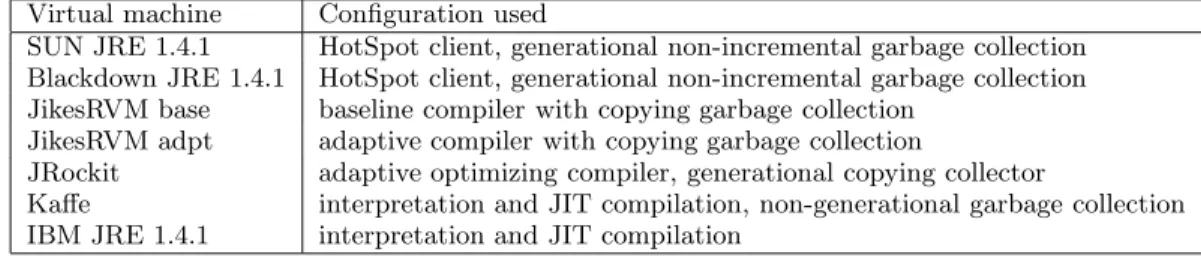
prin-cipal components that account for 86.5% of the observed variance in the measurements of the 49 Java workloads (7 SPECjvm98 benchmarks times 7 VM configurations). The factor loadings obtained for the principal components are given in Figure 1. These factor loadings account for 46.1%,
-1 -0.8 -0.6 -0.4 -0.2 0 0.2 0.4 0.6 0.8 1 in s tr o p s br b r_ ta k e n fa r_ c tr l re t ic _ fe tc h ic _ m is s ic _ L 2 _ fe tc h ic _ m e m it lb _ L 1 _ m is s it lb _ L 2 _ m is s fe tc h _ s ta ll b r_ m p re d b r_ ta k e n _ m p re d re t_ m p re d ta rg e t_ m p re d ra s _ h it s ra s _ o fl o w d is p a tc h _ s ta ll ic u _ fu ll re s _ s ta t_ fu ll fp u _ fu ll ls u _ fu ll ls u _ L 2 _ fu ll d c _ a c c e s s d c _ m is s d c _ L 2 d c _ m e m d c _ w b d tl b _ L 1 _ m is s d tl b _ L 2 _ m is s m e m _ re q u e s ts
principal component 1 principal component 2 principal component 3 principal component 4
general processor frontend branch prediction processor core data cache bus
Figure 1: Factor loading for SPECjvm98 with the s1 input set.
22.2%, 11.1% and 7.2% of the total variance, respectively.
When we take a closer look to the factor loadingsaij of the
retained principal components, it is obvious that the first component is by far the most important one. The contri-butions of the measured characteristics to the second, the third and fourth component are relatively smaller. In the following enumeration, we discuss the contributions made by each of the performance characteristics to each principal component:
• The main positive influence on the first principal
com-ponent (P C1) is caused by the branch prediction
char-acteristics and processor frontend charchar-acteristics, with except for the amount of fetch stalls, see Table 4. The first principal component is negatively influenced by several stall events, i.e., the amount of fetch stalls, dispatch stalls, ICU full stalls and L2/memory LSU full stalls. In addition,P C1 is also negatively affected
by the number of data cache misses, data cache write-backs and data cache refills from L2 and from mem-ory. Finally,P C1 is also negatively influenced by the
amount of memory requests seen on the bus.
• The second principal component (P C2) is positively
influenced by the number of x86 instructions retired per clock cycle and the number of retired operations per cycle, the amount of retired near return instruc-tions, the number of stalls caused by a full L1 LSU unit, and the amount of data cache accesses. This component is negatively influenced by the number of instruction fetches from memory, by the number of L2 I-TLB misses, by the branch prediction accuracy and by the number of stalls caused by full reservation sta-tions. It is also negatively influenced by the number of L1 D-TLB misses.
• For the third principal component (P C3), we see that
the amount of (taken) branches as well as the number of stalls caused by full reservation stations deliver the major positive contributions. P C3 is negatively
influ-enced by the amount of retired far control instructions, the amount of L1 I-TLB misses that hit the L2 I-TLB, and the amount of L2 D-TLB misses.
• The fourth principal component (P C4) is the
posi-tively dominated by the amount of L1 D-TLB misses that hit in the L2 D-TLB, and negatively dominated by the amount of branches and the amount of L2 D-TLB misses.
The factor loadings also give an indication of the corre-lated characteristics for this set of Java workloads. For ex-ample, from these results we can conclude that (along the first principal component) the branch characteristics corre-late well with the frontend characteristics. Moreover, this correlation is a positive correlation since both characteristics have a positive contribution to the first principal component. Also, the frontend characteristics correlate negatively with the amount of fetch stalls. In other words, this implies for example that a high number of I-cache fetches per unit of time correlates well with a low number of fetch stalls per unit of time which can be understood intuitively.
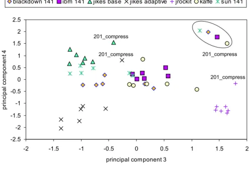
We can now display these Java workloads in the 4-dimen-sional space built up by the four principal components. This is shown in Figures 2 and 3 for the first versus the second principal component and the third versus the fourth prin-cipal component, respectively. Since we are dealing with a four-dimensional space, it is important to consider these two plots simultaneously to get a clear picture of the four dimen-sions. Note that in Figures 2 and 3, different SPECjvm98 benchmarks running on the same virtual machine are all represented by the same symbol. These graphs should be
-1.5 -1 -0.5 0 0.5 1 1.5 2 2.5 -2.5 -2 -1.5 -1 -0.5 0 0.5 1 1.5 principal component 1 p ri n c ip a l c o m p o n e n t 2
blackdown 141 ibm 141 jikes base jikes adaptive sun 141 kaffe jRockit
201_compress
201_compress 201_compress 201_compress
Figure 2: Scatterplot for the SPECjvm98 s1 workload set, as a function of the first and the second principal component. Different SPECjvm98 benchmarks running on the same virtual machine are represented by the same symbol. -2.5 -2 -1.5 -1 -0.5 0 0.5 1 1.5 2 2.5 -2 -1.5 -1 -0.5 0 0.5 1 1.5 2 principal component 3 p ri n c ip a l c o m p o n e n t 4
blackdown 141 ibm 141 jikes base jikes adaptive jrockit kaffe sun 141
201_compress
201_compress 201_compress
201_compress
Figure 3: Scatterplot for the SPECjvm98 s1 workload set, as a function of the third and the fourth principal component. Different SPECjvm98 benchmarks running on the same virtual machine are represented by the same symbol.
interpreted as follows. A Java workload having a high coef-ficient along the first principal component shows a behavior that can be characterized by, see also Figure 1, high numbers for the branch characteristics and the frontend characteris-tics. In addition, low numbers will be observed for several stall characteristics (fetch, dispatch, ICU and L2/memory LSU), the number of data cache misses, the number of data refills from L2 and memory, the number of data writebacks, and the number of memory requests from the bus.
The graphs in Figures 2 and 3 clearly show that the data points are more or less clustered per virtual machine. In-deed, we observe tight clusters for JRockit, the baseline ver-sion of Jikes, the adaptive verver-sion of Jikes and the IBM 1.4.1 VM. The clusters corresponding to the SUN 1.4.1 VM and the Blackdown 1.4.1 VM, are clustered less tightly. Notice also that these two clusters are quite close to each other. This is obviously due to the fact that both virtual machines are built around the same HotSpot virtual machine core. This graph also reveals that Kaffe exhibits the least tightly
clustered behavior. From these results we can conclude that
for the s1 input set, the virtual machine has a larger im-pact on the overall behavior than the Java application. In other words, a virtual machine running a Java application with a small input will exhibit similar behavior irrespective of the Java application it is running. This can be under-stood intuitively since thes1input set results in very short running benchmarks (in the order of seconds) for which the startup time of the virtual machine (initializing and loading significant parts of the JDK library) is the highest factor
contributing to the overall behavior. From these data we
can also conclude that using thes1input set of SPECjvm98 in a performance analysis might not be a good method unless one is primarily interested in measuring startup times, not just long-running performance.
It is also interesting to note that the data points corre-sponding to the 201 compress benchmark are not part of the clusters discussed in the previous paragraph. In other words, for this Java benchmark, the interaction between the application and the virtual machine has a large impact on its overall behavior at the microarchitectural level since the var-ious virtual machines for 201 compress are spread over the Java workload space. A close inspection of 201 compress re-veals that it has a small code size, while processing a fairly large amount of data, even in case of thes1input set. Profil-ing shows that for this benchmark, the top 10 methods that are called, account for 98% of all method calls. Clearly, 201 compress has a small number of hot methods, much smaller than the other SPECjvm98 benchmarks. This leads to a small working set and allows fairly aggressive optimiza-tions by the virtual machine’s native code generator. Since each virtual machine implements its run-time optimizer in a different way, this can result in a behavior that is quite different for each virtual machine. Note however that the SUN 1.4.1 VM, the Blackdown 1.4.1 VM and the IBM 1.4.1 VM yield quite similar behavior for 201 compress.
Another way of visualizing the (dis)similarity in this trans-formed space after PCA can be obtained through cluster analysis (CA). A dendrogram can be displayed which graph-ically represents the linkage distance during CA. This den-drogram is shown in Figure 4. In a denden-drogram, data points connected through small linkage distances are clustered in early iterations of the algorithm and thus exhibit similar be-havior. In our case, Java workloads exhibiting similar
behav-ior will thus be connected through small linkage distances. Based on Figure 4, we can make the same conclusions as we made based on the visualization of the reduced space obtained after PCA, see Figures 2 and 3. For example, we clearly observe the four tight clusters per virtual machine: (i) the baseline Jikes virtual machine, (ii) the adaptive Jikes virtual machine, (iii) the JRockit virtual machine, and (iv) the IBM 1.4.1 virtual machine. Also, we clearly observe that the SUN 1.4.1 and the Blackdown 1.4.1 VMs are loosely clustered. In addition, the Kaffe virtual machine results in the least tight cluster. Finally, concerning 201 compress, we observe that the Java workloads are linked through large linkage distances, and that a tight cluster is observed for the SUN 1.4.1 VM, the IBM 1.4.1 VM and the Blackdown 1.4.1 VM running 201 compress.
4.1.2
Analysis of the s100 input set
For thes100input set, we retain six principal components
after PCA that account for 87.3% of the observed variance in the measurements. These six principal components ac-count for 48.4%, 16.3%, 8.1%, 6.5%, 4.3% and 3.7% of the total variance, respectively. Note that the first four compo-nents account for 79.2% of the variance which is less than the variance explained by the four principal components for
s1. This indicates that the data for s100 are not as much
correlated as fors1. The factor loadings have the following contibutions from the various characteristics.
• For the first principal component (P C1), there are
pos-itive contributions, mainly from the number of retired x86 instructions per cycle, the number of L1 and L2 I-cache fetches, the branch prediction accuracy, and the number of D-cache accesses. Negative contributions come from the number of fetch stalls and dispatch stalls, the number of D-cache misses, the number of D-cache writebacks and the number of requests made to memory as seen on the bus.
• For the second principal component (P C2), positive
contributions are made by the number of FPU full stalls, the amount of D-cache accesses, and the num-ber of x86 retired instructions per cycle; while negative contributions are made by the branch prediction accu-racy and the number of L1 D-cache misses.
• For the third principal component (P C3), there is a
single important positive contribution made by the number of branches. A negative contribution is made by the number of return address stack (RAS) overflows and the number of L1 LSU full stalls.
• The fourth component is positively influenced by the
number of L1 D-TLB misses and the number of retired far control transfers. It is negatively influenced by the number of mispredicted indirect branches, the number of mispredicted near returns and the number of RAS overflows.
• The fifth component is positively dominated by the
number of instruction fetches from memory and nega-tively dominated by the number of ICU full stalls.
• The sixth and last retained principal component is
positively influenced by the number of I-fetches from the L2 cache and the number of L1 I-cache misses.
0.0 0.5 1.0 1.5 2.0 2.5 3.0 3.5 4.0
Jikes base Jikes adaptive + Jikes base, 201_compress Jikes adaptive JRockit Kaffe 222_mpegaudio, 227_mtrt JRockit 201_compress IBM Kaffe 228_jack Kaffe 202_jess, 209_db, 213_javac SUN Blackdown 222_mpegaudio, 227_mtrt SUN Blackdown 201_compress 202_jess, 209_db 213_javac, 228_jack
Figure 4: Dendrogram for the SPECjvm98 s1 workload set obtained after cluster analysis using the average pair-group strategy.
0 1 2 3 4 5
Sun + Blackdown + IBM + Jikes adaptive 213_javac, 228_jack
Jikes adaptive 202_jess, 227_mtrt 201_compress
SUN + Blackdown 202_jess JRockit
Kaffe 213_javac, 228_jack Jikes base 222_mpegaudio 209_db SUN + Blackdown 228_jack Kaffe 209_db, 227_mtrt
Kaffe 213_javac IBM 202_jess Sun + Blackdown + IBM 227_mtrt
Figure 5: Dendrogram for the SPECjvm98 s100 workload set obtained after cluster analysis using the average pair-group strategy.
The component in negatively influenced, mainly by the number of retired taken branches, the number of re-tired near returns, and the number of RAS hits. Although the reduced 6-dimensional space obtained after PCA is significantly smaller than the original 34-dimensional space, displaying a 6-dimensional space in an understand-able way is impractical, if not impossible. Therefore, we only display the dendrogram obtained after CA and not the Java workload space as a function of its principal components. This dendrogram is shown in Figure 5. A first interesting observation that can be made from this figure is that the
clusters that are formed for thes100input set are not the
same as fors1, compare Figure 5 to Figure 4. Moreover, the
clusters that are formed fors100are not necessarily formed
around virtual machines as it was the case for thes1input
set.
For thes100 input set, we observebenchmark clusters—
the same benchmark being run on different VMs, or small
impact of VM on overall behavior—as well as virtual
ma-chine clusters—the same virtual machine running different Java applications, or large impact of VM on overall behavior. In Figure 5,we observe three tight benchmark clusters: (i) a cluster corresponding to 201 compress, (ii) a cluster corre-sponding to 222 mpegaudio, and (iii) a cluster correspond-ing to 209 db. The first two clusters contain all the virtual machines except for the baseline version of Jikes. The last cluster around 209 db contains five virtual machines, all but Kaffe and the baseline version of Jikes. Interestingly, Shuf et al.[23] labeled these SPECjvm98 benchmarks as ‘simple’ benchmarks. The fact that the virtual machines running these ‘simple’ benchmarks result in clustered data points is probably (and surprisingly) due to the fact that all the vir-tual machines have optimized these simple benchmarks to nearly the same native code during the long-running time of these benchmarks. Note that in contrast to the widespread
behavior of 201 compress for thes1 input, the s100 input
results in a tight cluster.
In addition to these three ‘benchmark clusters’, we
ob-serve two tight virtual machine clusters: (iv) the baseline version of the Jikes virtual machine, and (v) the JRockit virtual machine. The cluster around the baseline Jikes VM contains all the SPECjvm98 benchmarks. The fact that the various Java programs that are run on baseline Jikes exhibit similar behavior can be explained as follows. The baseline configuration of Jikes compiles each method just-in-time but the number of (dynamic) optimizations performed is limited. As such, we can expect that more or less the same code se-quences will be generated for different Java programs yield-ing similar behavior. The cluster around JRockit contains all the SPECjvm98 benchmarks except for 201 compress, 209 db and 222 mpegaudio. Interestingly, these benchmarks are part of the ‘benchmark clusters’ (i), (ii) and (iii).
From a close inspection of the results in Figure 5,we also observed that the SUN 1.4.1 VM and the Blackdown 1.4.1 VM yield similar behavior. Note however, in contrast to the results ofs1, that this is only true on a per benchmark basis.
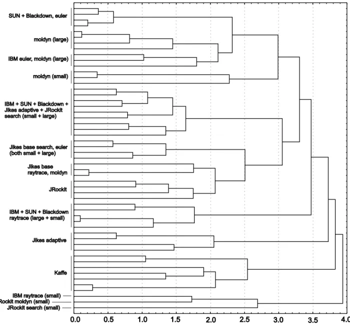
4.2
Java Grande Forum
For the Java Grande Forum (JGF) benchmark suite, which includes four benchmarks each having two problem sizes see also Table 2, we retain six principal components during PCA. These six principal components explain 82.5% of the total variance. The dendrogram obtained from cluster
anal-ysis on this 6-dimensional space is shown in Figure 6. From this figure, we can conclude that (i) the Java workloads as-sociated with Kaffe as well as the Java workloads asas-sociated with the baseline configuration of Jikes form tight clusters, respectively; (ii) a tight cluster is observed for search: all
the virtual machines runningsearchare in the same cluster
except for Kaffe and the baseline version of Jikes; (iii) the SUN 1.4.1 VM and the Blackdown 1.4.1 VM also show simi-lar behavior per benchmark, e.g., both virtual machines are
close to each other for the eulerbenchmark; (iv) the small
and large problem sizes generally yield the same behavior except formoldyn.
4.3
All the Java workloads
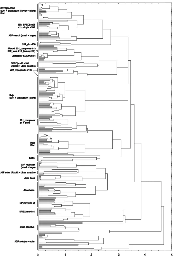
For the analysis discussed in this section, as much as 227 Java workloads are included by varying the virtual machine, the Java application and their input sets. Next to the vir-tual machine configurations mentioned in Table 1, we added the server mode of the SUN 1.4.1 VM as well as the server mode of the Blackdown 1.4.1 VM. Based on the results of the principal components analysis we retain seven princi-pal components accounting for 82.2% of the total variance. The dendrogram obtained from the cluster analysis done on this 7-dimensional space is shown in Figure 7. Interesting observations can be made from this figure.
• First, a number of virtual machine clusters are
ob-served that contain various Java applications on the same virtual machine, (i) the IBM 1.4.1 VM running the Raja benchmark, (ii) the Jikes baseline configura-tion, (iii) Kaffe, running several Java Grande Forum benchmarks and some SPECjvm98 benchmarks for the
s100input set, (iv) the adaptive configuration of Jikes, and (v) minor clusters for JRockit and the IBM VM. Note that the SUN 1.4.1 VM and the Blackdown 1.4.1 VM form a single cluster for the Raja benchmark as well as for SPECjbb2000, indicating strong similari-ties in the behavior of both virtual machines for these benchmarks. For SPECjbb2000, although the client and server modes of the SUN and Blackdown virtual machines are quite close to each other in the global picture (linkage distance smaller than 1.2), we can ob-serve a clear distinction between both. In addition, we also noticed that for SPECjbb2000, the server mode Blackdown 1.4.1 VM shows more similarities with the IBM 1.4.1 VM than with the server mode SUN 1.4.1 VM.
• Second, we observe a number of benchmark clusters
containing various virtual machines running the same Java benchmark, e.g, the Java Grande Forum
bench-marks (search, moldyn, euler and raytracer),
SPEC-jvm98’s 201 compress, SPECSPEC-jvm98’s 209 db with the
s100input and SPECjbb2000.
• Third, we observe two clusters formed around several
of the SPECjvm98 benchmarks with thes1input set,
showing once more that these workloads exhibit dis-similar behavior from the other Java workloads. How these results should be interpreted and used by re-searchers in the object oriented programming community
depends on their research goals. Virtual machine
0.0 0.5 1.0 1.5 2.0 2.5 3.0 3.5 4.0 SUN + Blackdown, euler
moldyn (large)
IBM euler, moldyn (large)
moldyn (small)
IBM + SUN + Blackdown + Jikes adaptive + JRockit search (small + large)
Jikes base search, euler (both small + large)
Jikes base raytrace, moldyn
JRockit
IBM + SUN + Blackdown raytrace (large + small)
Jikes adaptive
Kaffe
JRockit search (small) JRockit moldyn (small)
IBM raytrace (small)
Figure 6: Dendrogram for the Java Grande Forum benchmarks obtained after cluster analysis using the average pair-group strategy.
SPECjbb2000
SUN + Blackdown (server + client) IBM
IBM SPECjvm98 s1 + single s100
JGF search (small + large)
209_db s100 JRockit 201_compress (s1) 202_jess, 213_javac(s100) JRockit SPECjvm98 s1
SPECjvm98 s100 JRockit + Jikes adaptive 222_mpegaudio s100
Raja
SUN + Blackdown (client)
201_compress s1 + s100 Raja IBM Kaffe JGF raytracer (small + large) JGF euler JRockit + Jikes adaptive Jikes base Jikes base SPECjvm98 s1 SPECjvm98 s1 Jikes adaptive JGF moldyn + euler 1 2 3 4 5 0
Figure 7: Dendrogram for all the Java workloads obtained after cluster analysis using the average pair-group strategy.
0 2 4 6 8 10 201_compress 202_jess 227_mtrt 222_mpegaudio 209_db 0 2 4 6 8 10 linkage distance 213_javac 228_jack 228_jack with parallel GC 213_javac with parallel GC
Figure 8: Measuring the impact of the garbage col-lector on Java workload behavior.
a number of benchmarks that cover a sufficiently large be-havioral spectrum for their virtual machine. The collec-tion of benchmarks will thus be different for different vir-tual machines. For example, for JRockit we recommend SPECjbb2000, 201 compress, 222 mpegaudio, 228 jack, 213 javac, 209 db and the four JGF benchmarks. For the baseline configuration of Jikes on the other hand, we rec-ommend only two SPECjvm98 benchmarks and one JGF
benchmark. Java application developers benchmarking their
own Java program are recommended to use a sufficiently large number of virtual machines. However, our results sug-gest that it is a waste of effort to consider the SUN VM as well as the Blackdown VM.
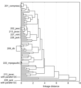
4.4
Comments on the garbage collector
As noted in section 2.1.1, the choice of the garbage col-lector was not consistent, i.e., different virtual machine con-figurations have different garbage collectors. This was due to the fact that we have chosen the default garbage col-lector for each virtual machine. To quantify the impact of the choice of the garbage collector on the overall results of this paper, we have set up the following experiment. We
considered the SPECjvm98 benchmarks with the s100
in-put set for the various virtual machine configurations in Ta-ble 1. For the JRockit VM we considered three additional garbage collectors next to the generational copying garbage collector, namely single spaced concurrent, generational con-current and parallel garbage collection. The dendrogram that is obtained after PCA and CA is shown in Figure 8. The four JRockit garbage collectors are highlighted for each SPECjvm98 benchmark. This graph shows that for most benchmarks the various garbage collectors are tightly clus-tered, except for the parallel garbage collector for 213 javac and 228 jack. As such, we conclude that the choice of the
garbage collector in this paper has a minor influence on the overall conclusions of this paper.
5.
RELATED WORK
This section discusses related work on understanding and characterizing Java workloads.
Bowers and Kaeli [8] characterize the SPECjvm98 bench-marks at the bytecode level. They conclude that Java ap-plications have a large number of loads in their dynamic bytecode stream.
Hsiehet al.[15] compare the performance of the SUN JDK
1.0.2 Java interpreter, a bytecode to native code translator called Caffeine [16] and a compiled C/C++ version of the code. This is done based on simulations. They conclude that the interpreter exhibits poor branch target buffer (BTB) performance, poor I-cache behavior and poor D-cache be-havior compared to the other approaches.
Chowet al. [10] compare Java workloads with non-Java workloads (e.g., SPEC CPU95, SPEC CINT95, etc.) using principal components analysis. In this study, the authors focus on the branch behavior, i.e., the number of conditional jumps, direct calls, indirect calls, indirect jumps, returns, etc. Based on simulation results, they conclude that Java workloads appear to have more indirect branches than non-Java workloads. However, the number of indirect branch targets can be small. I.e., when considering the number of indirect target changes, Java workloads are no worse than some SPEC CINT95 benchmarks. The study presented in
this paper is different from the work done by Chow et al.
for three reasons. First, although Chow et al. use a large
number of workloads, the number of virtual machines used in their study is limited to two. Second, Chowet al.limit their study to the branching characteristics of Java workloads.
Third, the goal of the paper by Chowet al.was the compare
Java workloads versus non-Java workloads which is different from the goal of this paper, namely getting insight in the interaction between VMs, Java programs and their inputs.
Radhakrishnanet al.[20, 21] analyze the behavior of the
SPECjvm98 benchmarks by instrumenting the virtual ma-chines and by simulating execution traces. They used two virtual machines: the Sun JDK 1.1.6 and Kaffe 0.9.2. They conclude that (i) 45 out of the 255 bytecodes constitute 90% of the dynamic bytecode stream, (ii) an oracle translation scheme (optimal translation selection) in case of a JIT com-piler can only improve performance by 10% to 15%, (iii) the I-cache and D-cache performance is better for Java applica-tions than for C/C++ applicaapplica-tions, except for the D-cache in JIT mode, (iv) write misses due to installing JIT compiler output have a significant impact on the D-cache performance in JIT mode, and (v) the amount of ILP is higher under JIT mode than under interpreter mode.
Liet al.[19] characterize the behavior of SPECjvm98 Java benchmarks through complete system simulation. This was done by using the Sun JDK 1.1.2 virtual machine and the SimOS complete system simulator [22]. They conclude that the SPECjvm98 applications (on s100) spend on average 10% of their time in system (kernel) activity compared to only 2% for the four SPEC CINT95 benchmarks studied. Generally, the amount of time in kernel activity is higher for the JIT compiler mode than for the interpreter mode. The kernel activity is mainly due to TLB miss handler invoca-tions. Also, they conclude that the SPECjvm98 benchmarks have inherently poor instruction-level parallelism (ILP)