An Exercise in Declarative Modeling
for Relational Query Mining
Sergey Paramonov, Matthijs van Leeuwen, Marc Denecker, and Luc De Raedt KU Leuven, Celestijnenlaan 200A, 3001 Heverlee - Belgium,
Abstract. Motivated by the declarative modeling paradigm for data mining, we report on our experience in modeling and solving relational query and graph min-ing problems with the IDP system, a variation of the answer set programmmin-ing paradigm. Using IDP or other ASP languages for modeling appears to be natu-ral given that they provide rich logical languages for modeling and solving many search problems and that relational query mining (and ILP) employs the same type of representation.
Nevertheless, our results indicate that second order extensions to these languages are necessary for expressing the model as well as for efficient solving, especially for what concerns subsumption testing. We propose such second order extensions and evaluate their potential effectiveness with a number of experiments in sub-sumption as well as in query mining.
Keywords: knowledge representation, answer set programming, data mining, query mining, pattern mining
1
Introduction
In the past few years, many pattern mining problems have been modeled using con-straint programming techniques [1]. While the resulting systems are not always as effi-cient as state-of-the-art pattern mining systems, the advantages of this type of declara-tive modeling are now generally accepted: they support more constraints, they are easier to modify and extend, and they are built using general purpose systems. However, so far, the declarative modeling approach has not yet been extended to inductive logic programming. This paper investigates whether such an extension would be possible. To realize this, we consider frequent query mining, the ILP version of frequent pat-tern mining, as well as the answer set programming paradigm, the logic programming version of constraint programming. More specifically, we address the following three questions:
Q1 Is it possible to design and implement a declarative query miner that uses a logical and relational representation for both the data and the query mining problem? Q2 Is it possible to take advantage of recent progress in the field of computational logic
by adopting an Answer Set Programming (ASP) [2] framework for modeling and solving?
Q3 Would such a system be computationally feasible? That is, can it tackle problems of at least moderate size?
Our study is not only relevant to ILP, but also to the field of knowledge representation and ASP as query mining (and ILP) is a potentially interesting application that may introduce new challenges and suggest solver extensions.
More concretely, the main contributions of this work can be summarized as follows: 1. We present two declarative models and corresponding solving strategies for the query mining problem that support a variety of constraints. While one model can be expressed in the ASP paradigm, the other model requires a second order extension that we believe to be essential for modeling ILP tasks.
2. We implement and evaluate the presented models in the IDP system [3], a knowl-edge base system that belongs to the ASP paradigm.
3. We empirically evaluate the proposed models and compare them on classical datasets with state-of-the-art ILP methods.
This paper is organized as follows: Section 2 formally introduces the problem. In Section 3, we introduce a second order model for frequent query mining that addresses Question Q1. In Section 4 we present a first order model for query mining, demon-strate main issues with this approach and address QuestionQ2. In Section 5 we provide experimental evidence to support our answers to QuestionsQ2 andQ3. In Section 6 we discuss advantages (such as extendability) and disadvantages of the models and the approach overall. In Section 7 we present an overview of the related work in the ILP context of frequent query mining. Finally, we conclude in Section 8 with a summary.
2
Problem statement
The problem that we address in this paper is to mine queries in a logical and relational learning setting. Starting with the work the Warmr system [4], there has been a line of work that focusses on the following frequent query mining problem [5, 6, 7]:
Given:
– a relational databaseD,
– the entity of interest determining thekeypredicate, – a frequency thresholdt,
– a languageLof logical queries of the formkey(X) ← b1, ..., bn definingkey/1
(bi’s are atoms).
Find:all queriesc∈ Ls.t.freq(c, D)≥t, wherefreq(c, D) =|{θ|D∪c|=key(X)θ}|. Notice that the substitutionsθonly substitute variables that appear in the conclusion part of the clause, i.e., only for variablesXthat occur inkey.
In this paper, we focus our attention on graph data, as this forms the simplest truly relational learning setting and allows us to focus on what is essential for extending the declarative modeling paradigm to a relational setting. In principle, this setting can easily be generalized to the full inductive logic programming problem.
As an example, consider a graph databaseD, represented by the facts
{edge(g1,1,2), edge(g1,2,3),edge(g1,1,3),edge(g2,1,2), edge(g2,2,3), edge(g2,1,3), . . .}, where the ternary relationedge(g, e1, e2)states that in graphgthere is an edge between
e1ande2(we assume graphs to be undirected, so there is also always an edge between
in this database is 2 as the query returnsg1andg2. Ifkey(g)holds, then the graphgis subsumed by the query specified defined in the body of the clause forkey.
The goal of this paper is to explore how such typical ILP problems can be encoded in ASP languages. So, we will need to translate the typical ILP or Prolog construction into an ASP format. In the present paper, we employ IDP, which belongs to the ASP family of formalisms. Most statements and constraints written in IDP can be translated into standard ASP mechanically. A brief example-based introduction to IDP is in Appendix A and for a detailed system and paradigm description we refer to the IDP system and language description [3] and to the ASP primer [2].
To realize frequent query mining in IDP, we need to tackle four problems: 1) encode the queries in IDP; 2) implement the subsumption test to check whether a query sub-sumes a particular entity in the database; 3) choose and encode a language bias; and 4) determine, in addition to frequency, further constraints that could be used and encode them. We will now address each of these problems in turn.
3
Encoding
We assume that the datasetDis encoded as two predicates:edge(g, e1, e2), described before, and the ternary relationlabel(g, n, l)that states that there is a nodenwith label
lin graphg(for a discussion on how to extend this approach, see Section 6) .
Encoding a query The coverage test in ILP is oftenθ- orOI-subsumption.
Definition 1 (OIandθ-subsumption [8]).A clausec1θ-subsumes a clausec2iff there
exists a substitution θsuch thatc1θ ⊆ c2. Furthermore,c1 OI-subsumesc2iff there
exists substitutionθ such that com(c1)θ ⊆com(c2), where com(c) = c∪ {ti 6= tj | tiandtjare two distinct terms in c}.
As ASP and, in particular, IDP are model-generation approaches, they always generate a set of ground facts. This implies that ultimately the queries will have to be encoded by a set of ground facts foredgeandlabelas well (e.g.,{edge(q,77,78), edge(q,77,79), label(q,77, a), label(q,78, b), label(q,79, c), . . .}) and that we need to explicitly en-code subsumption testing, rather than, as in Prolog, simply evaluate the query on the knowledge base. We use the convention that if a quantifier for a variable is omitted, then it is universally quantified. Furthermore, we use the convention that variables start with an upper-case and constants with a lower-case character. To illustrate the idea, consider the program in Eq. 1 that has a model if and only if the queryq OI-subsumes the graphg. If we remove the last constraint in Eq. 1, we obtainθ-subsumption. Notice that the functionθwill be explicit in the model. This program can be executed in IDP directly.
edge(q, X, Y) =⇒ edge(g, θ(X), θ(Y)). label(q, X, L) =⇒ label(g, θ(X), L).
X 6=Y =⇒ θ(X)6=θ(Y).
(1)
Notice that, in theory, it would be possible to simply encode subsumption testing in IDP or ASP as rule evaluation. That is, in the above example, to assert the knowledge base and the rule definekeyand then to ask whetherkey(g)succeeds. Computationally,
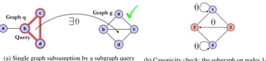
(a) Single graph subsumption by a subgraph query
(inq(x)in red) (b) Canonicity check: the subgraph on nodes 1-3-4 ismapped to 1-2-4 (lexicographically smaller)
Fig. 1: Examples of single graph subsumption (left) and of a canonicity check (right)
this would however be infeasible as the sizes of the grounded rules grow exponentially with the number of distinct variables in the rule.
Throughout the paper we use OI-subsumption for all tasks, except for the exper-imental comparison with Subsumer in Section 5 (since it is not designed to perform OI-subsumption).
Encoding the language bias In practice, one often bounds query languages, for instance by using a bottom clause and only considering queries or clauses that subsume the bottom clause.
Definition 2 (Language bias of a bottom clause⊥).Let⊥be a clause that we call bottom, then the language biasLis a set of clauses:L={c|cOI-subsumes⊥}.
This approach also works for ASP. We select one graph from the data and the set of all atoms in that instance will serve as bottom clause⊥. When fixing such an instance, we can encode queries by listing the nodes in that entity that will be present in the pattern using the unary predicateinq(x)(forin query), as visualized in Figure 1a.
We now present a modification of the previous encoding in Eq. 1 that takes into account the selection of the subgraph of the picked graphqas a query (marked in red in Figure 1a). We refer to the edges in the bottom clause asbedgeand labels in the bottom clause asblabel. When we refer to a node in the bottom clause, we call it abnode.
inq(X)∧inq(Y)∧bedge(X, Y) =⇒ edge(g, θ(X), θ(Y)). inq(X)∧blabel(X, L) =⇒ label(g, θ(X), L). inq(X)∧inq(Y)∧X 6=Y =⇒ θ(X)6=θ(Y).
(2)
The intuition behind these rules is that we select a subgraph by picking nodes in the bottom clause (i.e., a graph), and then we enforce the constraints on the nodes that have been selected. Eq. 2 implements this by adding aninqpredicate at the beginning of each clause as a guard, the rule is activated iff the corresponding node is selected.
Encoding the multiple subsumption test In frequent query mining one is interested in miningfrequentqueries, which implies that there is a bag of graphs to match.
Figure 2a illustrates this setup. We can see that we need to test whether the query
θ-subsumes each of the graphs in the dataset. To do so, we quantify over a function representingθ, the homomorphism. This makes this formulation second order. Why do we quantify over a function here and not in the previous example? Before the function was quantified existentially since the whole program was asking for a model, which is the same as asking whether the functions exists. Here however, we need a separate function for each graph, since the reasoning process is going to take into account the existence and non-existence of homomorphisms for particular graphs and to reason on
top of that.
homo(G)⇐⇒ ∃θ: bedge(X, Y)∧inq(X)∧inq(Y) =⇒ edge(G, θ(X), θ(Y)). blabel(X, L) =⇒ label(G, θ(X), L).
X 6=Y =⇒ θ(X)6=θ(Y).
(3) This constraint mimics the single graph subsumption test but introduces a new predicate
homo, indicating a matched graph.
We refer to the group of constraints in Eq. 3 asMatching-Constraint. The syntax used above is not yet supported by ASP-solvers such as clasp [9] or IDP [3], but we will argue that adding such second order logic syntax is crucial to enable effective modeling and solving of any structural mining problem. This argument will be backed up by experiments in Section 5.
Encoding the frequency constraint We consider two typical query mining settings: fre-quent and discriminative query mining. In the frefre-quent setting a query is accepted if it subsumes at least tgraphs. In the discriminative setting, each graph in the dataset is labeled as either positive or negative, as indicated by the corresponding predicates
positive(G)(negative(G)) that marks a positive (negative) graphG, and we are inter-ested in queries that match more thantpgraphs with a positive label and do not match
more thantnnegatively labeled graphs.
To model the frequent setting we use an aggregation constraint (Eq. 4) and the discriminative setting can be modeled similarly (Eq. 5):
|{G:homo(G)}| ≥t. (4)
|{G:positive(G)∧homo(G)}| ≥tp∧ |{G:negative(G)∧homo(G)}| ≤tn. (5)
Encoding the canonical form constraint It is well-known since the seminal work of Plotkin [10] that the subsumption lattice contains many clauses that are equivalent, and there has been a lot of work in ILP devoted to avoid the generation of multiple clauses from the same equivalence class (e.g., the work on optimality of refinement operators [11] and many others [12, 13]).
This can be realized in ASP by checking that the current query is not isomorphic to a lexicographically smaller subgraph (using a lexicographic order on the identifiers of the entities or nodes). For example, in Figure 1b, consider the subgraph induced by the nodes 1-3-4 (the numbers are identifiers and the colors are labels). Notice that there is an isomorphic subgraph 1-2-4, i.e., there exists a functionθpreserving edges and labels such that a string representation of the latter subgraph is smaller than the former. We call the graph with the smallest lexicographic representationcanonical. Canonicity can
be enforced by the following group of constraints, calledCanonical-Form-Constraint. ¬∃θ X6=Y =⇒ θ(X)6=θ(Y).
inq(X)⇐⇒ ∃Y :θ(X) =Y.
inq(X)∧inq(Y)∧bedge(X, Y)⇐⇒bedge(θ(X), θ(Y)). inq(X)∧blabel(X) =Y ⇐⇒blabel(θ(X)) =Y. inθ(Y)⇐⇒θ(X) =Y. d1(X)⇐⇒inq(X)∧ ¬inθ(X). d2(X)⇐⇒inθ(X)∧ ¬inq(X). min(d1(X))>min(d2(X)) . (6)
We refer to this group of constraints asCanonical-Form-Constraint. It enforces a query to have the smallest lexicographic representation, like the canonical code of mining algorithms [6, 7]. We define a canonical representation in terms of the lexicographic or-der over the bottom clause node identifiers. If there is a query satisfying the constraints, then there is no other lexicographically smaller isomorphic graph.
Note: Intuition on Eq. 6The first four rules ensure the existence of a homomorphism under OI-assumption (which can be relaxed by removing a constraint) between the cur-rent query on the node ininqand another subgraph of the bottom clause. The other rules ensure that the other subgraph has a smaller lexicographic order:inθ is an aux-iliary predicate that stores nodes of the other subgraph, ind1(d2) there are nodes that only belong to the first, current query, (or second) subgraph. If the minimal node ind1 (current query) is larger than ind2(the other graph), the query is not in canonical form. We now present additional types of constraints that allow solving variations of the query mining problem.
Connectedness-Constraint As in graph mining [6], we are often only interested in con-nected queries. The constraint to achieve this consists of two parts: 1) a definition of path and 2) a constraint over path. The first is defined inductively over the bnodes se-lected byinq(X), the second enforces that any two nodes in the pattern are connected. Note, that the usage of{. . .}indicates an inductive definition: the predicate on the left side is completely defined by the rules specified between curly brackets as a transitive closure. If both variables are in the pattern, there must be a path between them.
{path(X, Y)←inq(X)∧inq(Y)∧bedge(X, Y).
path(X, Y)← ∃Z :inq(Z)∧path(X, Z)∧bedge(Z, Y)∧inq(Y). path(Y, X)←path(X, Y).}
inq(X)∧inq(Y)∧X 6=Y =⇒ path(X, Y).
(7)
The Objective-Function An objective function is one way to impose a ranking on the queries. A constraint in the form of an objective function is defined over a model to maximize certain parameters. We consider only objective functions over the queries and matched graphs in the dataset: 1) no objective function, i.e., the frequent query mining problem; 2) maximal size of a query Eq. 8 (in terms of bnodes); 3) maximal coverage Eq. 9 (i.e., the number of matched graphs); 4) discriminative coverage Eq. 10,
i.e., the difference between the number of positively and negatively labeled graphs that are covered by a query.
|{X:inq(X)}| 7→max (8)
|{G:homo(G)}| 7→max (9)
|{G:positive(G)∧homo(G)}| − |{G:negative(G)∧homo(G)}| 7→max (10) Mining the top-k queries with respect to a given objective function is often a more meaningful task than enumerating all frequent queries, since it provides a more man-ageable number of solutions that are best according to some function [14].
Topological-Constraint Enforces parts of the bottom clause to be in the query. LetX be the desired subset of the nodes, then the constraint isV
X∈Xinq(X).
Cardinality-Constraint This constraint ensures that the size of a graph pattern is at least
n(at most, equal)∃ ◦n X :inq(X), where◦ ∈ {=,≤, <,≥, >}.
If-Then-Constraint This constraint ensures that if a node is present in the query, then another node must be present in the query, e.g., a nodeY must be present in the query, if a nodeXis in. We encode this constraint as a logical implication:inq(X) =⇒ inq(Y).
4
First Order Model
(a) Frequent query mining
(b) First order version of the graph mining model Fig. 2: Conceptual comparison between first and second order models
In the previous section we have given a positive answer to QuestionQ1using second order logic. However, after formalizing a problem the next step is to actually solve it. In this section we address QuestionQ2: can we use existing ASP solvers to model the frequent query mining problem directly? Is it necessary to add constructs to existing modeling languages, or is it possible to write down an efficient and elegant first order logic model for which existing solvers can be used?
To answer QuestionQ2, we will encode the problem of frequent query mining as an ASP problem using enumeration techniques. We shall also show how to approach top-k
The matching and occurrence constraints Since we are restricted to FOL here, we have to encodeθas a binary predicate, adding graphGas a parameter. In the encoding there are five clauses: the first enforces edge preservation; the second enforces that a mapping exists only for the bnodes in the pattern and only for the matched graphs, i.e.,θ(G, X)
is a partial function; the third enforcesθ(G, X)to be an injective function on the bnodes for each of the graphs; the fourth enforces label matching; the fifth ensures occurrence frequency (the same as before).
homo(G)∧inq(X)∧inq(Y)∧bedge(X, Y) =⇒edge(G, θ(G, X), θ(G, Y)). homo(G)∧inq(X)⇐⇒ ∃Y :Y =θ(G, X).
homo(G)∧inq(X)∧inq(Y)∧X 6=Y =⇒θ(G, X)6=θ(G, Y). homo(G)∧inq(X)∧blabel(X, L) =⇒label(G, θ(G, X), L).
|{G:homo(G)}| ≥t.
(11)
Encoding the model enumeration constraints A common technique in existing clause learning solvers with restarts for generating all solutions, is by asserting for each found solution a model invalidating clause which excludes this model. We use it to denote that certain combinations of nodes in the bottom clause are no longer valid solutions. E.g., if we find a graph on nodes 1-2-3 to be a solution and we store these nodes, then we prohibit this combination of nodes to ensure that the solver will find a new solution.
We present a version ofmodel invalidation clauses (MIC)[15] for frequent query enumeration. OurMICs are designed for Algorithm 1, since we enumerate queries of a fixed length: once we increase the length we remove all previousMICs. This allows us to useMICs of a very simple form: given a set of nodesX, we define a constraintCX
asCX =VX∈Xinq(X). For example, if a queryqon the nodes 1-2-3 is found to be
frequent, we would generate the following constraint, so not to generate 1-2-3 again:
inq(1)∧inq(2)∧inq(3).Note, that this simple form of model invalidation clauses can only be used if an algorithm iterates over the length of a query and removesMICs once the length is increased.
Anti-monotonicity property It is easy to integrate avoidance of infrequent supergraph generation in Algorithm 1: once a query is established to be infrequent, the correspond-ingMICis kept, when the query length is increased. However, our experiments in Sec-tion 5 indicate that the current computaSec-tional problems come from a different source and cannot be solved using this property.
Frequent query enumeration in Algorithm 1 We enumerate all frequent queries starting from the smallest ones (with only 1 node) to the largest ones (the bottom clause). Al-gorithm 1 has two loops. The first sets the current query size and setsMICto be empty (since we do not want to prohibit generation of supersets of already found queries). In the inner loop, we obtain a candidate for a frequent query by calling IDP once, then we check if the query is in canonical form and also obtain all isomorphic queries to this canonical form. After that we generate aMICfor each of them and prohibit the whole isomorphic class of queries to be generated. Note that generating all isomorphic queries is prohibitive, that is why we obtain a canonical query and remove all other isomorphic queries. The algorithm terminates if either it cannot find a new frequent query of any size or the required number of queries has been enumerated.
Algorithm 1First Order Model: Iterative Query Enumeration
Input:D, k, t .Dataset, #Queries, Threshold
Output:queries– set of frequent queries queries← ∅
⊥ ←pick-language-bias(D) .Language bias obtained from data maxsize←#nodes(⊥)
i←0
forsize∈1. . .maxsizedo
MICs← ∅
whileTruedo
query←mine-query(D,⊥, t,size,MICs) .IDP call, Eq. 11
ifqueryis Nonethen
break .the line below: IDP call, adopted Eq. 6 canonical,isomorphic←get-canonical-and-isomorphic(query,⊥)
queries←queries∪ {canonical} MICs←MICs∪isomorphic i←i+ 1
ifi≥kthen returnqueries
returnqueries
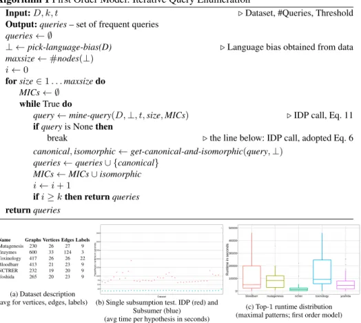
Name Graphs Vertices Edges Labels Mutagenesis 230 26 27 9 Enzymes 600 33 124 3 Toxinology 417 26 26 22 Bloodbarr 413 21 23 9 NCTRER 232 19 20 9 Yoshida 265 20 23 9
(a) Dataset description (avg for vertices, edges, labels)
● ●●● ● ● ● ● ● ● ● ●●●●●●●● ●●● ●● ●● ●●●●●●●●●●● ● ● ●● ● ●●●●●●●●●●●●●●●●●●●●●●●●●●●●●●●●●●●●●●●●●● 25 50 75 100 150 200 250 300 350 Dataset Hypothesis r untime in seconds
(b) Single subsumption test. IDP (red) and Subsumer (blue)
(avg time per hypothesis in seconds)
● ● ● ● ● ●● 0 10000 20000 30000 40000 50000
bloodbarr mutagenesis nctrer toxinology yoshida
Runtime in seconds
(c) Top-1runtime distribution
(maximal patterns; first order model)
Fig. 3: Dataset description and the summary of subsumption and top-1experiments
Top-k problem Current ASP solvers, including IDP, can perform optimization de-scribed in Constraints 8, 9 and 10. However, Algorithm 1 enumerates patterns with respect to their size and therefore needs to be modified. The key change is to remove the outer for loop with the size variable together withCardinality-Constraint. In the experiment section we demonstrate that even top-1is already excessively complex for modern ASP solvers and requires further investigation and development of the systems.
5
Experiments
In this section we evaluate the encoding on three problems: 1) classicalθ-subsumption performed by IDP as encoded in Eq. 1, 2) the first order model in Algorithm 1 on the frequent query mining task, and 3) the first order model on the top-1 query mining task. In all experiments the frequency thresholdtis set to5%. Since the task involves making a stochastic decision, i.e., pick-language-bias in Algorithm 1 picks a graph from the dataset at random, this may significantly influence the running time. To resolve this issue, for the graph enumeration problem we average over multiple runs for each dataset: each run involves the enumeration of many queries, i.e., each run generates
many data points (runtimes to enumerateN queries). For the top-one mining problem, we present multiple runs for each dataset, since each run computes only one data point (runtime for the top-1query).
Subsumption We evaluate how the IDP model 1 encoding ofθ-subsumption compares with subsumption engine The Subsumer [16]. We used the data from the original Sub-sumer experiments (transition phase on the subsumption hardness [8, p. 327]) and eval-uated IDP subsumption programs and Subsumer on a single hypothesis-example test, i.e., for each hypothesis and example we have made a separate call to IDP and Subsumer to establish subsumption.
The goal of this experiment is to compare how both systems perform if computa-tions are done on a single example. We would like to estimate the potential gain in IDP, if we could specify a homomorphism existence check for each graph independently, like in a higher-order model Eq. 3, i.e., for each graph we would check existence of someθ(X)instead of checking existence of one functionθ(G, X)like in the first order model.
Figure 3b indicates that IDP and Subsumer perform within a constant bound when we make a separate call for each example and hypothesis. That is, for all but one dataset, the runtimes are within the same order of magnitude for the two methods. If the internal structures of the system are reused and the call is made only for one hypothesis perset
of examples, we observe a speedup of at least one order of magnitude in Subsumer. This indicates that the system is able to efficiently use homomorphism independence. Once the solver community will have built extensions of systems like IDP to take advantage of homomorphism independence, the resulting systems will perform substantially bet-ter than the current ones and their performance will be close to that of special purpose systems such as Subsumer. More precisely, systems should exploit that it is computa-tionally easier to findnfunctionsθ(X), than oneθ(G, X)fornvalues ofG.
Datasets and implementation We now evaluate the query mining models on a number of well-known and publicly available datasets: Blood Barrier, NCTRER and Yoshida datasets are taken from [17], Mutagenesis and Enzymes datasets are from [18], Toxi-nology dataset is from [19]. A summary of the dataset properties is presented in Table 3a.
Top-1performance evaluation We present the results of evaluating the FOL model for top-1 mining in Figure 3c. Results were only obtained for the maximal size, and no solutions were computed for Enzymes in a reasonable time (<10h). The discriminative setting cannot be modeled and solved, since we need higher order primitives and for maximal coverage we already experienced an explosion of the search space. This exper-iment demonstrates that current satisfiability solvers cannot effectively perform search on both categories of query variables and homomorphism coverage; solver extensions are necessary. The first extension is to specify independence of the homomorphisms in the model, i.e., higher order primitives as indicated in the model Eq. 3, the second is to give more control over the solver’s decisions, e.g., by allowing to specify a decision order.
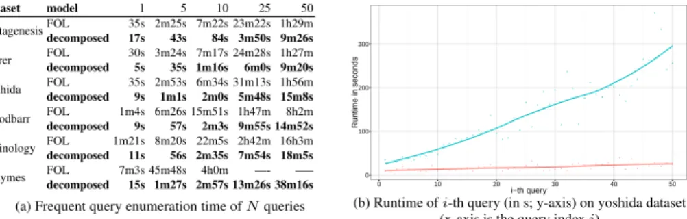
Frequent query mining The goal of the next experiment is to estimate the potential gain of the introduction of a higher order modeling construction. To do this, we mimicked the higher order behavior in Algorithm 1 by making several calls to IDP (one per graph)
in the methodmine-query. We call this mimicking modeldecomposed. The results of the evaluation are presented in Figure 4a, a comparison of the decomposed and the original FOL model are in Figure 4b. Homomorphism dependence in the first order model causes serious computational difficulties, which makes higher order primitives one of the main priorities for solving query mining. The runtime also grows with the size of a pattern since it affects the search space and runtime as a result.
dataset model 1 5 10 25 50 mutagenesisFOL 35s 2m25s 7m22s 23m22s 1h29m decomposed 17s 43s 84s 3m50s 9m26s nctrer FOL 30s 3m24s 7m17s 24m28s 1h27m decomposed 5s 35s 1m16s 6m0s 9m20s yoshida FOL 35s 2m53s 6m34s 31m13s 1h56m decomposed 9s 1m1s 2m0s 5m48s 15m8s bloodbarr FOL 1m4s 6m26s 15m51s 1h47m 8h2m decomposed 9s 57s 2m3s 9m55s 14m52s toxinology FOL 1m21s 8m20s 22m5s 2h42m 16h3m decomposed 11s 56s 2m35s 7m54s 18m5s enzymes FOL 7m3s 45m48s 4h0m —- —– decomposed 15s 1m27s 2m57s 13m26s 38m16s
(a) Frequent query enumeration time ofNqueries
●● ● ● ●●●● ● ● ● ●●●● ● ●● ● ● ●● ● ● ● ● ● ●●●● ● ●●● ● ●●● ● ● ● ● ● ●● ● ● ●● ● ●● ●●● ●● ● ● ●● ● ● ● ● ● ● ● ● ●● ● ● ● ● ● ● ● ● ● ● ● ● ● ● ● ● ●● ● ● ● ● ●● ● ● ● ● 0 100 200 300 0 10 20 30 40 50 i−th query Runtime in seconds
(b) Runtime ofi-th query (in s; y-axis) on yoshida dataset
(x-axis is the query indexi)
Fig. 4: Frequent query enumeration FOL (blue) vs decomposed model (red)
Summary of the experimental results The results show that the model performs rea-sonably and we therefore conclude that it can be considered a first step towards the development of declarative languages for relational query mining. From Figure 3b and 4a it is clear that the core computational difficulty lies in the inability to state homomor-phism independence. This follows from the candidate generation and canonicity check runtime and from the speedup that Subsumer has when it is applied to the whole set of examples with one call. After comparing the performance of IDP and Subsumer on a single example and observing the speed up of the decomposed model in Figure 4a, one would expect a significant speedup if it were implemented within the solver.
We have observed in Figure 3c that query mining introduces interesting compu-tational challenges and might be of interest to the solver development community as well as to the ILP community. We also pointed out the reasons for these computational difficulties and suggested possible ways to enhance the solvers.
6
Model discussion and generalization
Advantages and disadvantages of the model There is a number of advantages of the declarative approach to pattern mining compared to the classical imperative methods: compact and clear representation; extendability and generality; provability and formal semantics of the models; and reliable and portable implementation (the solvers are de-veloped by the community, well tested and already applied to a variety of tasks; the solvers are available for all popular operation systems: Linux, MacOS, and Windows).
In particular, our model compactly represents not only the model of the graph min-ing problem but also the code that can be executed to solve the problem. Addmin-ing the source code of gSpan [20] to a paper (∼ 2000lines of C++) would be impossible. Also, the model allows easy extension by adding constraints to the theory, e.g., adding a constraint to handle labels on edges is just an extra line with a straightforward logi-cal formula. Last but not least our formulation allows formal rigorous reasoning on the constraints that constitute the model.
These advantages come, of course, at a cost. Typically, specialized algorithms per-form an order of magnitude (at least) faster. The main reason for such a speed up is that most mining algorithms incorporate and heavily rely on the structure of the problem in the search strategy. Our experiments in Figure 4b demonstrate that the declarative approach can reduce the runtime gap by extending the language to better incorporate the structure of a problem. Also, modeling this kind of mining problems influences the way declarative solvers are built and potentially can lead to better solving system that would perform reasonable on mining problems.
Generalization of the approach Let us demonstrate how the model can be extended to handle labels on the edges as an example of how declarative systems can be adapted to solve new tasks.
Assume that edge labels are represented using the predicateedgelabel(g, e1, e2, l) and the edge labels of the bottom clause are stored in the predicatetedgelabel(e1, e2, l). Then, the first order formulation Eq. 11 can be extended by adding the constraint:
inq(X)∧inq(Y)∧tedgelabel(X, Y, L) =⇒ edgelabel(G, θ(G, X), θ(G, Y), L).
Intuitively, this constraint ensures that if there is an edge(X, Y)with a labelLin the bottom clause, then there is an edge with a labelLin the graphG. If each edge has a label, the constraint above can replace the first constraint in Eq. 11.
The smallest change, according to the principle, is the addition of a rule or a fact. In general, this example demonstrates how our declarative approach and our model in particular implements the elaboration tolerance principle [21], i.e., a small change in the problem formulation should lead to a small change in the model. The smallest changes, according to the principle, is the addition of a rule or a fact. With this respect our model satisfies the elaboration tolerance principle and can be called an additive elaboration.
7
Related work
WARMR [4] and FARMER [6] are extensions of the Apriori algorithm for discovering frequent structures in multiple relations. Even though they use ILP techniques (e.g., a declarative language bias) to determine frequent queries, they imperatively specify computations and the algorithm does not support the addition of arbitrary constraints due to the restricted nature of the algorithm, and hence focuses on a specific task. B-AGM, Biased-Apriori-based Graph Mining [5], is another system based on Apriori. C-Farmr [7] is an ILP system for frequent Datalog clauses that uses so-called condensed representations to avoid the generation of semantically equivalent clauses.
The XHAIL system [22] uses ASP as a computational engine to perform abductive inductive reasoning. It is similar in the way we use an ASP engine as computational core, but XHAIL is focused on the abduction task, whereas we focus on query mining which always involves aggregation and model enumeration.
In the work on sequence testing [23] ASP is used as a subroutine in a cycle and also model projection on a predicate is also present similarly to our Algorithm 1, but this similarity is technical, since the tasks are of different nature. ASP has also been applied to itemset mining [24] and sequence mining [25]; the presented results are preliminary, the suggested methods only deal with one particular task in its basic formulation.
gSpan [20] is a specialized algorithm designed to solve the frequent graph pattern mining problem. The algorithm is tailored to solve only one task exclusively and re-quires significant changes in its core to be extended to solve other mining tasks (and, to the best of our knowledge, there is no extension to the full relation setting). It is similar, however, in the computational challenges: canonicity checks, homomorphism checks, language bias, etc.
8
Conclusions
We have shown that modern ASP solvers can be applied to ILP query mining tasks. We have provided experimental evidence that these models can be used as prototypes for developing declarative mining languages. We have also indicated the reasons why the solvers need to be extended to make computation efficient and proposed concrete extensions as well as estimated their potential effectiveness. The query mining models and the experimental setup we developed provide an interesting challenge for the ASP solver developer community and a potentially useful tool for the ILP community.
References
[1] Tias Guns et al. “MiningZinc: A Modeling Language for Constraint-Based Mining”. In: IJCAI. 2013.
[2] Thomas Eiter, Giovambattista Ianni, and Thomas Krennwallner. “Answer Set Program-ming: A Primer”. In:5th International Reasoning Web Summer School (RW 2009), Brix-en/Bressanone, Italy, August 30 – September 4, 2009. Vol. 5689. 2009.
[3] Broes De Cat et al. “Predicate Logic as a Modelling Language: The IDP System”. In: CoRRabs/1401.6312 (2014).
[4] Ross D. King, Ashwin Srinivasan, and Luc Dehaspe. “Warmr: a data mining tool for chem-ical data.” In:Journal of Computer-Aided Molecular Design15.2 (2001), pp. 173–181. [5] Akihiro Inokuchi, Takashi Washio, and Hiroshi Motoda. “An Apriori-based Algorithm for
Mining Frequent Substructures from Graph Data”. In: 2000, pp. 13–23.
[6] Siegfried Nijssen and Joost N. Kok. “Efficient frequent query discovery in FARMER”. In: In Proc. of the 7th PKDD, volume 2838 of LNCS. 2003, pp. 350–362.
[7] Luc De Raedt and Jan Ramon. “Condensed Representations for Inductive Logic Program-ming”. In:KR. 2004, pp. 438–446.
[8] Luc De Raedt.Logical and Relational Learning: From ILP to MRDM (Cognitive Tech-nologies). Springer-Verlag New York, Inc., 2008.
[9] Martin Gebser et al. “clasp: A Conflict-Driven Answer Set Solver”. In:LPNMR. 2007, pp. 260–265.
[10] G. D. Plotkin. “A further note on inductive generalization”. In: volume 6 (1971), pages 101–124.
[11] S. Muggleton. “Inverse Entailment and Progol”. In:New Generation Computing, Special issue on Inductive Logic Programming13.3-4 (1995), pp. 245–286.
[12] Patrick R.J. van der Laag and Shan-Hwei Nienhuys-Cheng. “Completeness and proper-ness of refinement operators in inductive logic programming”. In:The Journal of Logic Programming34.3 (1998), pp. 201 –225.
[13] Jens Lehmann and Pascal Hitzler. “Foundations of Refinement Operators for Description Logics”. In:Inductive Logic Programming. Vol. 4894. 2008, pp. 161–174.
[14] Jilles Vreeken, Matthijs Leeuwen, and Arno Siebes. “Krimp: Mining Itemsets That Com-press”. In:Data Min. Knowl. Discov.23.1 (2011), pp. 169–214.
[15] Broes De Cat. “Separating Knowledge from Computation: An FO(.) Knowledge Base System and its Model Expansion Inference”. PhD thesis. KU Leuven.
[16] Jose Santos and Stephen Muggleton. “Subsumer: A Prolog theta-subsumption engine”. In: ICLP Technical Communications. Vol. 7. 2010, pp. 172–181.
[17] Ulrich R¨uckert and Stefan Kramer. “Optimizing Feature Sets for Structured Data”. In: ECML ’07. Warsaw, Poland, 2007, pp. 716–723.
[18] Asim Kumar Debnath et al. “Structure-activity relationship of mutagenic aromatic and het-eroaromatic nitro compounds. Correlation with molecular orbital energies and hydropho-bicity”. In:Journal of medicinal chemistry34.2 (1991), pp. 786–797.
[19] Christoph Helma and Stefan Kramer. “A Survey of the Predictive Toxicology Challenge 2000-2001.” In:Bioinformatics19.10 (2003), pp. 1179–1182.
[20] Xifeng Yan and Jiawei Han. “gSpan: Graph-Based Substructure Pattern Mining”. In: ICDM ’02. 2002.
[21] John McCarthy. “Elaboration Tolerance”. In: (1999).
[22] Oliver Ray. “Nonmonotonic Abductive Inductive Learning”. In:Journal of Applied Logic (2008).
[23] Esra Erdem et al. “Answer-Set Programming as a New Approach to Event-Sequence Test-ing”. In: Proc. of the 3rd International Conference on Advances in System Testing and Validation Lifecycle. 2011.
[24] Matti Jrvisalo. “Itemset Mining as a Challenge Application for Answer Set Enumeration”. In:LPNMR’11. 2011, pp. 304–310.
[25] Thomas Guyet, Yves Moinard, and Ren´e Quiniou. “Using Answer Set Programming for pattern mining”. In:CoRRabs/1409.7777 (2014).
A
Appendix: Introduction to IDP
Listing 1.1: IDP source code example – map coloring
vocabularyV{ typearea typecolor border(area,area) coloring(area):color } theoryT:V{
// Adjacent countries can not have the same color
∀A1A2:border(A1, A2) =⇒ coloring(A1) 6=coloring(A2).
}
structureS:V{
area={belgium; holland; germany; luxembourg; austria; swiss;france}
color={blue;red;yellow;green} border={ (belgium,holland);(belgium, germany);(belgium,luxembourg);(belgium,france); (holland,germany);(germany,luxembourg);(germany,austria);(germany,swiss); (germany,france);(luxembourg,france);(austria,swiss);(swiss,france) } }
The IDP language [3, 15] is an extension of first order logic with inductive definitions and aggregration. The IDP system implements finite satisfiability and can be considered as an ASP system.
The particular type of inference we use in our work ismodel expansion. The task of model expansion is to expand a finite interpretationSfor the subvocabularyV of a given logic theoryT to a model ofT. In the example above,V is the vocabulary of the map colouring problem i.e.area,color,border(area,area),coloring::area7→color;
S consists of 7 countries, 4 colours and a border relation between the countries;T is the constraint that two bordering countries cannot have the same color.
In this example, the model expansion task is to find an extension ofS, i.e. color-ingfunction, such that the constraint inT is satisfied, i.e. all bordering countries have different colours.
The example can be tried online (select file “Map Colouring”): adams.cs.kuleuven.be/idp/server.html.