Wayne State University Theses
1-1-2011
Probabilistic models for patient scheduling
Adel Alaeddini
Wayne State University,
Follow this and additional works at:http://digitalcommons.wayne.edu/oa_theses
Part of theComputer Sciences Commons, and theMedicine and Health Sciences Commons
This Open Access Thesis is brought to you for free and open access by DigitalCommons@WayneState. It has been accepted for inclusion in Wayne State University Theses by an authorized administrator of DigitalCommons@WayneState.
Recommended Citation
by
ADEL ALAEDDINI
THESIS
Submitted to the Graduate School
of Wayne State University,
Detroit, Michigan
in partial fulfillment of the requirements
for the degree of
MASTER OF SCIENCE
2011
MAJOR: COMPUTER SCIENCE
(Data Mining)
Approved by:
I acknowledge Dr. Chandan K. Reddy, my advisor in the Department of Computer Science for his guidance throughout my thesis. Also, I am very thankful to Dr. Farshad Fotouhi in the Department of Computer Science and Dr. Kai Yang (my Ph.D. thesis advisor) in the Department of Industrial Engineering for giving me an opportunity to pursue my Masters degree in Computer Science simultaneously with my Ph.D. in Industrial Engineering. Finally, I kindly appreciate the support of my family and friends.
Dedication ... ii
Acknowledgements ... iii
List of Tables ... vi
List of Figures ... vii
CHAPTER 1 INTRODUCTION ... 1
1.1. Relevant Background ... 2
1.1.1. Factors Affecting No-Shows and Cancellations ... 3
1.1.2. Population based Models ... 3
1.1.3. Individual based Models ... 4
1.2. Preliminaries... 6
1.2.1. Notations Used for the Probability of Disturbance Prediction Model ... 6
1.2.2. Binomial and Multinomial Logistic Regression ... 7
1.2.3. Beta and Dirichlet Distributions ... 8
1.2.4. Bayesian Update of Beta and Dirichlet Distributions ... 9
1.2.5. Hotelling's Distribution ... 11
CHAPTER 2 PREDICTING DISTURBANCES IN APPOINTMENT SCHEDULING THROUGH HYBRID PROBABILISTIC MODELING ... 13
2.1. The Proposed Algorithm for No-Show Prediction ... 13
2.2. Experimental Results ... 16
2.2.1. Data Preprocessing ... 16
2.2.2. Applying the Proposed Model to a Sample Patient ... 19
2.2.2.1. Time wise Analysis ... 22
2.3. Generalization of the Proposed Algorithm for No-Show and Cancellation Prediction ... 28
2.4. Experimental Results ... 31
2.4.1. Data Preprocessing ... 32
2.4.2. Applying the Proposed Model to a Sample Patient ... 33
2.4.2.1. Time wise Analysis ... 36
2.4.2.2. Patient wise Analysis ... 40
2.4.2.3. Discussion ... 42
CHAPTER 3 AN OPTIMIZATION MODEL FOR EFFECTIVE APPOINTMENT SCHEDULING IN THE PRESENCE OF DISTURBANCES ... 44
3.1. Introduction ... 44
3.2. The Proposed Optimization Model for Non-Sequential Scheduling ... 47
3.3. An Optimization Model for Including changing no-show probabilities and walk-in Patients ... 49
3.3.1. Results on Simulated Data ... 51
3.4. Generalization of the Proposed Model for Sequential Scheduling ... 53
3.4.1. Estimation of Demand ... 56
3.4.2. Results on Simulated Data ... 57
CHAPTER 4 CONCLUSIONS AND FUTURE DIRECTIONS ... 58
Appendix A -Gaussian Mixture Models (GMM) and Expectation Maximization (EM) Algorithm ... 59
References ... 61
Abstract ... 65
Autobiographical Statement ... 66
Table 1: Notations used for the proposed prediction model ... 6
Table 2: Data structure for the weighting factors ... 19
Table 3: Attendance record of a sample patient ... 20
Table 4: A sample logistic regression model fitted to the dataset ... 20
Table 5: Bayesian update of Beta distribution parameters ... 21
Table 6: The result of clustering the clinics based on their no-show, cancellation and show-up probabilities... 32
Table 7: Data structure and optimal value of the weighting factors ... 33
Table 8: No-show, cancellation and show-up record of a sample patient ... 34
Table 9: A sample multiple logistic regression model fitted to the dataset ... 34
Table 10: Bayesian update of Dirichlet distribution parameters ... 35
Figure 1: (a) The histogram of clinics no-show probability, (b) The result of clustering the clinics based on their no-show probabilities ... 18 Figure 2: Applying the proposed model for a sample patient :(a) Real record of attendance and
estimated probability of no-show using the proposed model (b) Prior and posterior of Beta distribution for modeling no-show ... 22 Figure 3: Mean Squared Error (MSE) of the other methods used for comparison ... 23 Figure 4: Proposed approach performance over patients: (a) estimated versus real probability of
no-show, (b) Absolute difference of estimated and real no-show probability ... 24 Figure 5: Logistic regression performance over patients: (a) estimated versus real probability of
no-show, (b) Absolute difference of estimated and real no-show probability ... 25 Figure 6: ARIMA (1,1,0) performance over patients: (a) estimated versus real probability of
no-show, (b) Absolute difference of estimated and real no-show probability ... 26 Figure 7: Mean squared error (MSE) of different methods used for comparison comparing
methods ... 27 Figure 8: Applying the proposed model for a sample patient: (a) changing parameters during
Bayesian update (b) prior distribution (c) posterior distribution ... 36 Figure 9: Mean Squared Error (MSE) of the studied methods for time-wise analysis ... 38 Figure 10: The performance of the proposed approach over different patients: estimated versus
empirical probability of no-show and cancellation ... 38 Figure 11: The performance of pure multinomial logistic regression over different patients:
estimated versus empirical probability of no-show and cancellation ... 39 Figure 12: The performance of pure Bayesian updating method over different patients: estimated
versus empirical probability of no-show and cancellation ... 40 Figure 13: Mean Squared Error (MSE) of the studied methods for patient-wise analysis ... 41 Figure 14: The performance of the proposed approach over different patients: estimated versus
empirical probability of no-show and cancellation ... 41 Figure 15: The performance of pure multinomial logistic regression over different patients:
Figure 17: The expected total profit of the proposed non-sequential and the original scheduling model under different no-show probabilities for different types of patients ... 52 Figure 18: The expected total profit of the proposed non-sequential and the original scheduling
model under number of demands ... 53 Figure 19: The expected total profit of the proposed sequential and the original scheduling model across a sequence of 40 patient calls ... 57
CHAPTER 1
INTRODUCTION
The problem of no-shows and appointments cancellation (individuals who do not arrive for or cancel their scheduled appointments) cause significant disturbance on the smooth operation of almost all scheduling systems [Bech 2005; Moore et al. 2001]. While the reasons for these no-shows, and cancellations might vary from previous experience to personal behaviors, several practitioners and researchers have often neglected this important realistic aspect of the scheduling problem. This thesis, considers the problem of effective scheduling by predicting such disturbances accurately from the historical data available and incorporating them into scheduling using a novel optimization model. Specifically, the applicability and usefulness of the proposed work is demonstrated on healthcare data collected from a medical center. Due to the vast amounts of cost and resources involved in medical healthcare centers, such disturbances can incur losses of hundreds of thousands of dollars yearly [Bech 2005; Hixon et al. 1999; Rust et al. 1995; Barron 1980]. Such disruptions not only cause inconvenience to the hospital management but also has a significant impact on the revenue, cost and resource utilization for almost all the healthcare systems. Hence, accurate prediction of no-show and cancellation probabilities and incorporating them into the scheduling system is a cornerstone for any non-attendance reduction strategy [Cayirli and Veral 2003; Ho and Lau 1992; Cote 1999; Hixon et al. 1999; Moore et al. 2001].
In this research, a hybrid probabilistic model is developed to predict the probability of no-shows and cancellations in real-time using logistic regression and Bayesian inference. In addition, a novel optimization model which can effectively utilize no-show probabilities for scheduling patients is also developed. The proposed prediction model uses both the general social and demographic information of the individuals and their clinical appointments attendance
records, and other variables such as the effect of appointment date, and clinic type. In the mean time, the scheduling model considers both scheduled and unscheduled patients (walk-in patients) simultaneously. It also formulates the effect of patients’ overflow from one slot to another. In addition, it takes into account the effect of patients’ assignment to undesired appointment time on no-show/cancellation probability.
The result of the proposed method can be used to develop more effective appointment scheduling [Chakraborty et al. 2010; Glowacka et al 2009; Gupta and Denton 2008; Hassin and Mendel 2008; Liu et al. 2009]. It can also be used for developing effective strategies such as selective overbooking for reducing the negative effect of disturbances and filling appointment slots while maintaining short waiting times [Laganga and Lawrence 2007; Muthuraman and Lawley 2008; Zeng et al 2010].
The organization of this thesis is as follows: the rest of this chapter discusses the relevant background and preliminaries of this research. Chapter 2 describes the proposed models for predicting disturbances in appointment scheduling and the results of applying the proposed models on data collected from a medical healthcare center. Chapter 3 presents the proposed optimization models for effective appointment scheduling in the presence of disturbances along with two simulated numerical examples. Finally, chapter 4 concludes our work and presents some future extensions of this study.
1.1. Relevant Background
There are wide varieties of techniques that can be used for the estimation of no-show and cancellation probabilities. First, the factors that can affect no-shows and cancellations are briefly discussed. Next, some of the related quantitative methods studied in this domain are presented.
1.1.1. Factors Affecting No-Shows and Cancellations
There have been a few studies that discussed the effect of patients’ personal information such as age, gender, nationality, and population sector on the no-show and cancelation probabilities [Bean and Talaga 1995; and Glowacka 2009]. Some researchers have also investigated the relationship between no-show probability and factors related to the previous (appointments) experience of the person such as number of previous appointments, appointment lead times, waiting times, appointment type, and service quality [Cynthia et al 1995; Garuda et al. 1998; Goldman et al 1982; Dreihera et al. 2008; Lehmann et al. [2007]. A few studies also considered the effect of personal issues such as overslept or forgot, health status, presence of a sick child or relative, and lack of transportation on missing appointments [Campbell et al 2000; Cashman et al. 2004]. This study will consider many of these factors in our proposed model and also consider the effect of personal behavior such as previous appointment-keeping pattern as discussed in [Dove and Karen 1981] in predicting no-shows.
1.1.2. Population based Models
Population based techniques mainly use a variety of methods drawn from statistics and machine learning which can be used for predicting no-shows and cancellations [Dove and Schneider 1981]. These methods use the information from the entire population (dataset) in the form of set factors, in order to estimate the probability of no-show, cancellation and show-up. Logistic regression is one of the most popular statistical methods in this category that is used for binomial and multinomial regression, which can predict the probability of disturbances by fitting numerical or categorical predictor variables in the data to a logit function (Hilbe [2009]). There has been some work using tree-based and rule-based models which create if–then constructs to
separate the data into increasingly homogeneous subsets, based on which the desired predictions of disturbances can be made [Glowacka et al. 2009]. The problem with these population based methods is that although they provide a reasonable estimate, they do not differentiate between the behaviors of individual persons, and hence cannot update effectively especially while using small datasets. Another problem with these methods is that once the model has been built adding new data has minor effect on the result especially when the size of initial dataset is much larger compared to the size of the new data. In chapter 2, we compare some of above methodologies with our proposed approach on real-world patient scheduling data.
1.1.3. Individual based Models
Individual based approaches are primarily time series and smoothing methods that are used for predicting the probability of a disruption in an appointment. These methods utilize past behaviors of individuals for the estimation of future no-show and cancellation probability. Time series methods forecast future events such as no-shows and cancellations based on the past events by using stochastic models. There are different types of time series models; the common three classes amongst them are: the autoregressive (AR) models, the integrated (I) models, and the moving average (MA) models. These three classes depend linearly on previous data [Brockwell 2009]. Combinations of these ideas produce autoregressive moving average (ARMA) and autoregressive integrated moving average (ARIMA) models. Smoothing is an approximating function that attempts to capture important patterns in the data, while leaving out noise or other fine-scale structures and rapid phenomena. Many different algorithms are used in smoothing. Some of the most common algorithms are the moving average, and local regression [Simonoff 1996]. Bayesian inference is a method of statistical inference in which some kind of evidence or observations are used to update its previously calculated probability such as improving the initial
estimate of disturbances probabilities [Bolstad 2007]. To use Bayes’ theorem, we need a prior distribution that gives our belief about the possible values of the parameter before incorporating the data. The posterior distribution is proportional to prior distribution times likelihood | :
(
p y)
g( ) (
p f y p)
g | ∝ × |
( 1-1) If the prior is continuous, the posterior distribution can be calculated as follows:
| |
| ( 1-2)
While individual based methods are fast and effective in modeling the behavioral (no-show) pattern of each individual, and work well with a small dataset, they do not use the predictive information from the rest of the population and hence do not provide a reliable initial estimate of no-show and cancellation probabilities which is especially important in our problem. In chapter 2, the performance of some of above methods will be compared with the proposed work.
As described above, each of population based and individual based approaches have some advantages and disadvantages. However, none of the studies in the literature have considered using these methods together in order to overcome their problems and improve their performance. In chapter 2, a hybrid probabilistic model will be developed that combines logistic regression as a population based approach along with Bayesian inference as individual based approach for no-show and cancellation prediction. To demonstrate its effectiveness, the proposed model will be compared to the representative algorithms from both population based and individual based approaches
1.2. Preliminaries
This Section introduces some of the preliminaries required to comprehend the proposed algorithm. First the notations used in the study are described. Next, some basics about logistic regression, Beta and Dirichlet distributions as the vital components of the proposed model are explained. Finally, more details about Bayesian update of Beta and Dirichlet distributions as the main procedure of the proposed algorithm for modeling the individual’s behavior are provided.
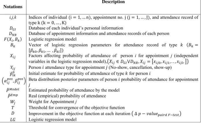
1.2.1. Notations Used for the Probability of Disturbance Prediction Model
Table 1 describes the notations used for the proposed prediction model.Table 1: Notations used for the proposed prediction model
Notations
Description
i,j,k Indices of individual i 1, … n , appointment no. j j 1, … , J , and attendance record of
type k k 0, … , K
Database of each individual’s personal information
Database of appointment information and attendance records of each person
, Logistic regression model
Vector of logistic regression parameters for attendance record of type , , … ,
Factors affecting probability of attendance of person i for appointment j (independent
variables in the logistic regression model), , , , . . , ,
Person attendance type for appointment (No-show, cancellation, show-up)
̂ Initial estimate for probability of attendance of type for person
, Beta distribution posterior parameters of person probability of attendance for appointment
Estimated probability of attendance by the model Real (empirical) probability of attendance
Weight for Appointment j
Threshold for convergence of the objective function
Improvement in the objective function at each iteration ∆
1.2.2. Binomial and Multinomial Logistic Regression
Logistic regression is a generalized linear model used for binomial regression, which predicts the probability of occurrence of an event by fitting numerical or categorical predictor variables in data to a logit function [Agresti 2002]:
⁄1 ( 1-3) where 0≤ p≤1 and
(
p 1− p)
is the corresponding odds. The logistic function can be written as:p=1+e−(β0+β1x1+...+βkxk)
1 ( 1-4) where prepresents the probability of a particular outcome. Given the set of explanatory variables and unknown regression coefficients βj,
(
0< j<k)
can be estimated using maximumlikelihood (MLE) methods common to all generalized linear models [Hilbe 2009].
Multinomial logistic regression is a generalization of the binomial model used when the dependent variable follows a multinomial distribution. The model then takes the form:
∑ , 1,2, … ,
∑
(1-5)
where is the probability of th event and is the vector of explanatory variables. The
unknown vector of parameters is typically estimated by the maximum a posteriori (MAP) estimation, which is an extension of maximum likelihood using regularization of the weights [Agresti 2002].
1.2.3. Beta and Dirichlet Distributions
Beta distribution: Beta
(
α,β)
represents a family of common continuous distributions defined on the interval [0,1] parameterized by two positive shape parameters, typically denoted by α and β with probability density function:
(
)
(
)
( ) ( )
1(
1)
1 , ; − − − Γ Γ + Γ = α β β α β α β α x x x f ( 1-6)where Γis the gamma function, and Γ
(
α + β) ( ) ( )
Γ α Γ β is a normalization constant to ensure that the total probability integrates to unity. The beta distribution is the conjugate prior of the binomial distribution. From the Bayesian statistics viewpoint, a Beta distribution can be seen as the posterior distribution of the parameter pof a binomial distribution after observing α −1 independent events with probability p and β −1 with probability 1− p, if there is no other information regarding the distribution of p [Evans et al. 2000].Dirichlet distribution (denoted by ) is the generalization of beta distribution to a family of continuous multivariate probability distributions parameterized by the vector α of
positive reals. The Dirichlet distribution of order 2 with parameters , . . . , 0 has a probability density function with respect to Lebesgue measure on the Euclidean space
given by [Evans et al. 2000]:
, . . , , , … , ∏ (1-7) for all γ , … ,γ 0 satisfying ∑ 1 (our work incorporates 3 which is based on the number categories: no-show, cancellation, and show-up). The density is zero outside this open 1 -dimensional simplex. The normalizing constant is the multinomial beta function, which can be expressed in terms of the gamma function:
∏∑ , , … , (1-8) Dirichlet distribution is the multivariate generalization of the beta distribution (multinomial distribution), and conjugate prior of the categorical distribution and multinomial distribution in Bayesian statistics. That is, its probability density function returns the belief that the probabilities of rival events given that each event has been observed 1 times.
1.2.4. Bayesian Update of Beta and Dirichlet Distributions
In Bayesian statistics, a Beta distribution [Bolstad 2007] is a common choice for updating a prior estimate of the Binomial distribution parameter p because:
1. A Beta distribution is the conjugate prior of a Binomial distribution (See Section 1.2.3). 2. Unlike a Binomial distribution, a Beta distribution is a continuous distribution, which is
much easier to work with in terms of inference and updating.
3. A Beta distribution has two parameters, which allows it to take different shapes, making it suitable for representing different types of priors.
If Beta
(
α,β)
is used as a prior, based on the conjugacy property of Beta distribution, theposterior would be a new Beta posterior with parameters α'=α +y and β'=β+n−y. In other words, Beta distribution can be updated simply by adding the number of successes yto αand
the number of failures n−y to β:
(
p y)
Beta(
y n y)
g | ~ α + ,χ + − ( 1-9)(
|)
(
(
) (
)
)
− −1(
1−)
− + −1 + − Γ + Γ + + Γ = α β β α β α py p n y y n y n y p g .( 1-10)As discussed earlier, individual-based approaches like empirical Bayesian inference will not be able to provide an initial estimate of the prior distribution. Hence, before applying the Bayesian update, the parameters of the prior distribution should be initialized.
[Bolstad 2007] suggests choosing parameters that match the belief about the location (mean) and scale (standard deviation) of the original distribution. Hence, if an initial guess of parameter
p is available, which in our study can be obtained from population-based approaches such as logistic regression, Beta distribution prior parameters can be computed by solving the following system of Equations for α and β .
(
)
(
)
⎪ ⎪ ⎩ ⎪⎪ ⎨ ⎧ + + − = − + = 1 1 1 β α β α α i i i i i p p n p p p ( 1-11)The point estimate of the posterior parameter pof the binomial distribution would be the mean of Beta distribution
β
α
α
+ of the updated Beta distribution.
Similarly, Dirichlet distribution is a regular option for updating prior estimate of Multinomial distribution parameters , … , . To use Bayes’ theorem, we need a prior distribution that gives our belief about the possible values of the parameter vector
, … , before incorporating the data.
Based on earlier discussion on Dir(α) , , … , can be used as prior density, which results in a new Dirichlet posterior with parameters vector , where is the number of occurrences of each category in the incorporated data. In other words, Dirichlet distribution can be updated simply by adding the new occurrence number of each category to the prior parameters :
| ∏∑ ∏ γ ( 1-12)
The posterior mean would then be | , … , ∑ ∑ with variance:
| , … , ∑ ∑
∑ ∑ ∑ ∑
(1-13)
For choosing an extended version of the procedure used for Beta distribution can be applied by letting ; where is the output of the multinomial logistic regression. As an alternative to above procedure, several researchers [Leonard 1973; Aitchison 1985; Goutis 1993; Forster and Skene 1994] proposed using a multivariate normal prior distribution for multinomial logits.
1.2.5. Hotelling's
Distribution
In statistics, Hotelling's statistic [Evans et al. 2000] is a generalization of Student's t -statistic that is used in multivariate hypothesis testing. Hotelling's -statistic is defined as follows:
(1-14)
where n is a number of points (see below), is a column vector of elements and W is a sample covariance matrix. If ~ , is a random variable with a multivariate Gaussian distribution and W~ , 1 (independent of ) has a Wishart distribution with the same non-singular variance matrix and 1, then the distribution of is, Hotelling's with parameters and n, where representing -distribution:
distribution can be used for pairwise comparison of the mean of two sets of multidimensional data : 0 against : 0, e.g. estimated and empirical probabilities of patient attendance. Above hypothesis can be tested using -statistic ~ , where
′ where and is calculated as follows:
∑ ( 1-16)
Also ∑ where ̂ , … , ̂ is the vector of
pairwise differences between person empirical and estimated probabilities for type
CHAPTER 2
PREDICTING DISTURBANCES IN APPOINTMENT
SCHEDULING THROUGH HYBRID PROBABILISTIC MODELING
2.1. The Proposed Algorithm for No-Show Prediction
Algorithm 1 illustrates the flow of the steps taken by the proposed approach for estimating no-show probability which can be categorized in three stages:
1. Initial no-show probability estimation 2. Bayesian update of the no-show estimate 3. Weight optimization
Algorithm 1: No-show Prediction Algorithm Input: Input data , , Threshold parameter
Output: Estimated no-show probability ̂ , Beta distribution posterior parameters , , Logistic regression estimated parameters
Procedure:
1 /* Logistic regression*/
2 Calculate MLE of Equation (1.4) parameters
3 ̂ 1| ,
4 , Solve system of Equation (1-11) with ̂ 1| 5 /*Weight optimization*/
6 ̂ ∑
1
7 Until Equation (2-1) improvement do
8 set a value for appointments weights
9 /*Bayesian update */ 10 , , , , 11 ̂ 12 ̂ ̂ 13 ∑ ̂ ̂ ∑ ̂ ̂ 1 14 ⁄ ⁄√ 15 Return ̂
In the first stage, based on the dataset of individuals’ personal information , (such as gender, marital status, etc.) and their sequence of appointment information (e.g. previous attendance records )), a logistic regression model , is formulated (line 2). Then, using logistic regression, an initial estimate of no-show probability is calculated, given by
p Y 1|X . As discussed in Section 1.1.2, Logistic regression bundles the information of the complete population together and finds a reliable initial estimate of no-show ( ̂ .
In the second stage, which is interlaced with the third stage, the initial estimate is used in a Bayesian update procedure to find the posterior no-show probability for each person. For this purpose, ̂ is transformed into prior parameters of a Beta distribution , as shown in
line 4. Next, using the attendance record of each person the posterior parameters
, and posterior probability of no show ̂ is calculated (lines 10 and 11). As discussed in Section 1.1.3, the reason Bayesian update procedure is applied to the output of logistic regression is that, typically regression models cannot consider individual patients behavior. Also, updating regression parameters based on new data records is both difficult and only marginally effective (especially when the model is already constructed on a huge dataset) in comparison to Bayesian update.
In the third stage, appointments are weighted based on on a subset of factors = , … ,
(line 8) to increase the model performance in estimating the real probability of no-show. An optimization procedure is used for finding the optimal value of the weights. The objective function of the model is to minimize the difference between the real and model estimated probability of no-show:
( )
0,1 ,..., : . max 1 1 , 2 0 1 , 2 0 ∈ ⎟ ⎟ ⎠ ⎞ ⎜ ⎜ ⎝ ⎛ > + ⎟ ⎟ ⎠ ⎞ ⎜ ⎜ ⎝ ⎛ − < = − − − − − ω α α w w T S t t p t t p value p n n test t paired ( 2-1)Where , … , are the weights to be optimized and value is the p-value of a two sided statistical hypothesis testing of the paired estimated p using the model and estimated p using the attendance records:
⎩ ⎨ ⎧ ≠ = Datal al D Model D Datal al D Model D p p H p p H Re 1 Re 0 : : ( 2-2)
It should be noted that the mean squared error ( ) can also be used as the objective function. However, t-statistics which is used above not only contains in itself ( in the denominator of t statistics is a linear function of ) (line 14), but also has a statistical distribution which makes it better choice for our optimization model.
In (2-1), , is the percentage of points or value of t random variables with n-1 degrees of freedom such that the probability that exceeds this value is , and
√
⁄ where ∑ ̂ ̂ ⁄ and is calculated as follows:
(
)
(
(
)
)
1 ˆ ˆ ˆ ˆ 1 2 1 Re 2 Re − ⎥⎦ ⎤ ⎢⎣ ⎡ − − − =∑
=∑
= n n p p p p S n i n i al i Model i al i Model i p ( 2-3) Where ̂ is the real rate of no-show for person calculated as ̂ ∑ , with as a binary (random) variable representing records of no-show/show of patient i for appointment j. Here, l is the index of first appointment in the validation dataset which is discussed shortly, andestimated no-show probability calculated based on weighted appointments using the proposed model.
The optimization procedure is as follows: at every iteration, a vector of weights is assigned to the appointments in validation dataset (line 8). The weighted appointments are then plugged into the Bayesian update mechanism for estimating the probability of no-show (lines 10 and 11). Next, the estimates of the proposed model and real attendance records are compared by forming a t- statistic (lines 12 to 14) and the p-value of the paired -test which shows the goodness of the assigned weights, is used for improving the initial set of weights (line 7) . This procedure continues until no improvement is observed. Then, the ̂ of the iteration resulted in the best value of objective function is used as the no show estimate.
2.2. Experimental Results
Here the proposed method is evaluated based on a healthcare dataset of 99 patients at the Veteran Affairs (VA) Medical Center in Detroit. The dataset includes the following data from patients’ personal and appointment information: (1) sex, (2) date of birth (DOB), (3) marriage status, (4) medical service coverage, (4) address (zip code), (5) clinic and (6) attendance record.
This Section is organized as follows: first data processing is discussed. Next, a stylized example for one patient is presented to show how the model works. Finally, the results of applying the model to the dataset is discussed using two types of analysis: one by defining training, validation and test dataset on patients, and one on appointment time.
2.2.1. Data Preprocessing
The data attributes in the dataset should be preprocessed before being used in the model. This includes: coding, dealing with missing attributes, and co-linearity elimination. Besides, because
of the variety of clinics (more than 150 in our case), if this explanatory variable gets directly used in the model, the accuracy of the logistic regression will be severely affected.
Such problem can be addressed by clustering similar clinics respect to their no-show rate. While various types of clustering algorithms can be used for this purpose, since the clinics are originally different in type, grouping them into a set of clusters will result in clusters with different density and dispersion. Such characteristics can be effectively considered using Generalized Mixture Models (GMM) [Alpaydim 2010].
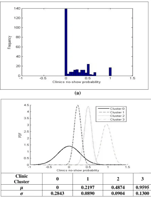
Figure 1(a) illustrates the histogram of clinics’ no-show probability and Figure 1 (b) shows the result of clustering the clinics based on their no-show probability using GMM. The final result which is four clusters has been verified by a team of experts.
(a)
(b)
Figure 1: (a) The histogram of clinics no-show probability, (b) The result of clustering the clinics based on their no-show probabilities
Also, (1) appointment recency, (2) appointment closeness to non-working days (Saturday, Sunday, and holidays), and (3) clinic cluster, are considered as weighting factors (
, , . Regarding the first factor, it is reasonable that no-show records that occurred long time ago do not carry the same weight as recent no-shows. This is based on the fact that patients may gradually or abruptly change their behavior, which should be reflected in the model.
Clinic
Cluster 0 1 2 3
0 0.2197 0.4874 0.9595
Regarding the second and third weighting factors, the study of data revealed a strong correlation among no-show rate and days close to holidays and clinic clusters.
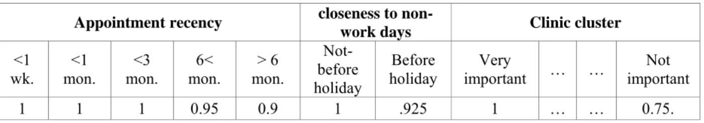
The weights discussed above are arranged in a special data structure before being applied to the data. For the appointment recency where more importance should be assigned to the recent appointments a logarithmic time framework with five weights is considered. For the appointment closeness to non-work days two weights are applied: one for Monday to Thursday and one for Friday and days before holidays. Finally, for clinics cluster, based on the groups derived using GMM, four weights are defined. Table 2 shows the final data structure and optimal value of the weights which is gained by solving Equation (2-1) using Genetic Algorithm (GA) algorithm.
Table 2: Data structure for the weighting factors
Appointment recency closeness to
non-work days Clinic cluster
<1 wk. <1 mon. <3 mon. 6< mon. > 6 mon. Not-before holiday Before holiday Very important … … Not important 1 1 1 0.95 0.9 1 .925 1 … … 0.75.
2.2.2. Applying the Proposed Model to a Sample Patient
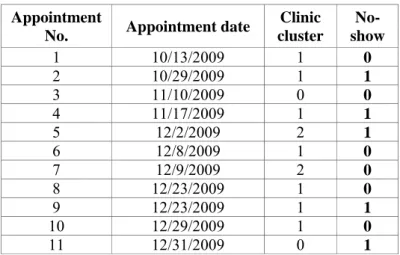
Here the procedure of no-show probability estimation for a randomly selected patient is explained. The selected patient is male, born on 02/5/1978, never married, degree of medical service coverage less than 5% with zip code 48235. Table 3 shows his appointment information as patterns of show/show from 10/13/2009 to 12/31/2009 (training dataset). Note that no-shows are represented by 1 while no-shows are represented by 0.
Table 3: Attendance record of a sample patient
Appointment
No. Appointment date
Clinic cluster No-show 1 10/13/2009 1 0 2 10/29/2009 1 1 3 11/10/2009 0 0 4 11/17/2009 1 1 5 12/2/2009 2 1 6 12/8/2009 1 0 7 12/9/2009 2 0 8 12/23/2009 1 0 9 12/23/2009 1 1 10 12/29/2009 1 0 11 12/31/2009 0 1
Using patient personal and appointment information as well as the attendance record, the parameters of the fitted logistic regression model are calculated in Table 4.
Table 4: A sample logistic regression model fitted to the dataset
Sex DOB Marriage
status Medical service coverage Zip code Clinic cluster Recency Closeness to non-workday Constant 71.6917 -0.8600 6.51E-05 -0.13596 0.0180 0.0015 0.4822 0 3.0410
Based on the estimated coefficients of logistic regression the probability of not showing up in the first appointment in the testing dataset (1/25/2010) is estimated as =0.3453. This estimate is used for building the prior Beta(0.3453,0.6547) of the Bayesian updating procedure by solving Equation (1-11). Table 5 illustrates the updated parameters of Beta distribution as well as the estimated probability of no-show after each appointment.
Table 5: Bayesian update of Beta distribution parameters Ap pointm en t No. Ap pointm en t da te C lin ic Ca teg ory Weight No-sho w We ig hted No-sho w Estimated p C lo sen es s to non -wo rkda y Recency Clin ic clu ster 0.3453 0.6547 0.345 12 1/25/2010 0 1 0.9 1 1 0.35 0.695 0.655 0.515 13 1/26/2010 1 1 0.9 0.9 0 0 0.695 1.655 0.296 14 2/2/2010 0 1 0.9 1 0 0 0.695 2.655 0.208 15 2/4/2010 2 1 0.9 0.75 0 0 0.695 3.655 0.160 16 2/6/2010 2 1 0.9 0.75 0 0 0.695 4.655 0.130 17 2/17/2010 0 1 0.9 1 0 0 0.695 5.655 0.109 18 2/18/2010 1 1 0.9 0.9 0 0 0.695 6.655 0.095 19 2/23/2010 0 1 0.9 1 0 0 0.695 7.655 0.083 20 3/2/2010 1 1 0.9 0.9 0 0 0.695 8.655 0.074 21 3/9/2010 0 1 0.9 1 1 0.35 1.045 8.655 0.108 22 3/16/2010 0 1 0.9 1 0 0 1.045 9.655 0.098 23 3/18/2010 2 1 0.9 0.75 0 0 1.045 10.655 0.089
As graphically illustrated in Figure 2 (a), the Bayesian update reacts quickly to each new data record, which means that the procedure can rapidly converge to the real distribution of no-show. Figure 2 (b) compares the prior and posterior distributions of no-show probability before and after applying testing data. It is easy to follow how the mass of the density function has moved to the left in the posterior which can be interpreted as decreasing the probability of no-show.
0 0.2 0.4 0.6 0.8 1 1 2 3 4 5 6 7 8 9 10 11 12 P ro b ab ilit y of no ‐ sh o w Appointment no. Estimated Probability of no‐ show Real record of attendance (a) (b)
Figure 2: Applying the proposed model for a sample patient :(a) Real record of attendance and estimated probability of no-show using the proposed model (b) Prior and posterior of Beta distribution for modeling no-show
2.2.2.1. Time wise Analysis
In this Section, the performance of the proposed model is compared with a number of population and individual based methods based on time wise analysis. In this regard the training, validation and testing data are defined as follows: appointments occurred before 6/31/2009 for
0 10 20 30 40 50 60 70 0 1 2 3 4 5 6 7 8 9 x pd f Prior Posterior
training, appointments between 6/31/2009 and 12/31/2009 for validation, and appointments after 12/31/2009 for testing. Such a setting is used for all of the time-wise experiments.
The comparing methods including: Box smoothing, autoregressive integrated moving average model (ARIMA), decision tree, and multiple logistic regression with same predictors as used in the proposed model regression part and rule-based methods. The moving window size of Box method is checked for the range of 1 to 7, where only 5 is considered. For ARIMA model two cases ARMA (1,1,0) and ARMA(2,2,0) are considered. Also, J48 and PART algorithms are used for building the decision tree rule-based methods.
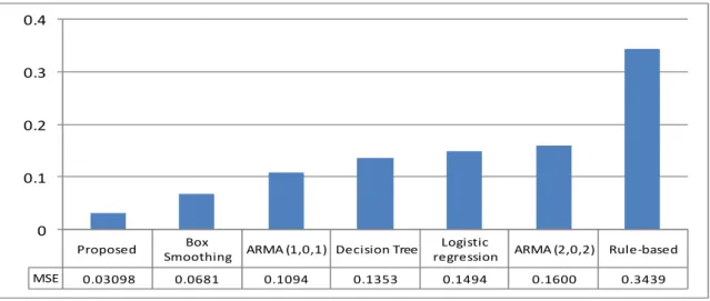
Figure 3 compares the Mean Squared Error (MSE) of the comparing methods. Based on MSE measure the proposed model performs clearly better than other methods while rule-based has the worst result. As can be seen from the results, in general, individual-based methods outperform population based methods, while bundling these methods together (as we have done in the proposed methods) significantly better method than both.
Proposed Box
Smoothing ARMA (1,0,1) Decision Tree
Logistic
regression ARMA (2,0,2) Rule‐based
MSE 0.03098 0.0681 0.1094 0.1353 0.1494 0.1600 0.3439 0 0.1 0.2 0.3 0.4
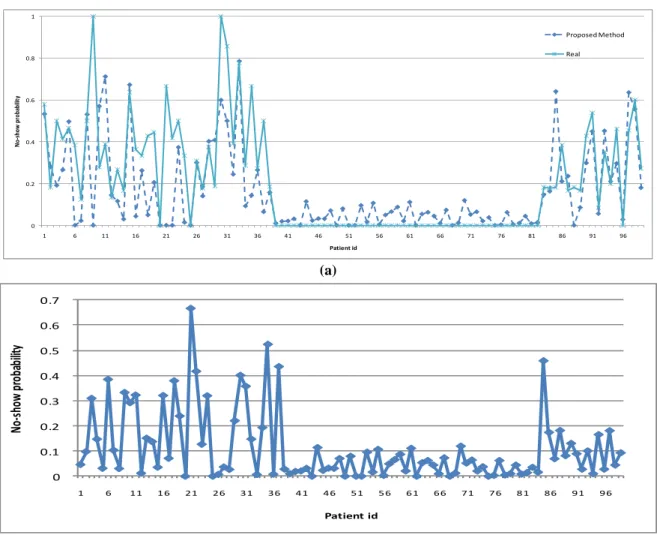
Figure 3: Mean Squared Error (MSE) of the other methods used for comparison Figures 4 to 6 illustrate some of the comparing methods estimates versus real probability of no-show over different patients. As can be seen from Figure 4 (a), the proposed approach
estimates often follows the real pattern correctly. This is better illustrated in Figure 4 (b) which shows the absolute difference between the estimated and real probability of no-show. Here, the mean of differences is 0.1104 which is acceptably low. There are also few cases with absolute difference more than 0.5. Later analysis reveals fewer available data records for those patients.
0 0.2 0.4 0.6 0.8 1 1 6 11 16 21 26 31 36 41 46 51 56 61 66 71 76 81 86 91 96 No ‐ sh ow pr ob ab ili ty Patient id Proposed Method Real (a) 0 0.1 0.2 0.3 0.4 0.5 0.6 0.7 1 6 11 16 21 26 31 36 41 46 51 56 61 66 71 76 81 86 91 96 No ‐ sh ow pr ob ab ilit y Patient id (b)
Figure 4: Proposed approach performance over patients: (a) estimated versus real
probability of no-show, (b) Absolute difference of estimated and real no-show probability Figure 5 (a) illustrates the estimates from one of the population based methods which is logistic regression. As can be seen, the estimates tend to have small fluctuations around an approximately fixed mean. Such result clearly shows that the regression models may not fully capture the difference among patients’ personal behaviors. The absolute difference between the
estimated and real probability of no-show which is shown in Figure 5 (b) also confirms similar results. Here the mean of the differences is 0.1935 while the maximum difference is 0.8683 which is considerable. Such a result is similar to other population based methods discussed earlier. 0 0.2 0.4 0.6 0.8 1 1 6 11 16 21 26 31 36 41 46 51 56 61 66 71 76 81 86 91 96 No ‐ sh ow pr ob ab ilit y Patient id Logistic Regression Real (a) 0 0.1 0.2 0.3 0.4 0.5 0.6 0.7 0.8 0.9 1 1 6 11 16 21 26 31 36 41 46 51 56 61 66 7 1 76 8 1 86 9 1 96 No ‐ sh ow pr ob ab ilit y Patient id (b)
Figure 5: Logistic regression performance over patients: (a) estimated versus real
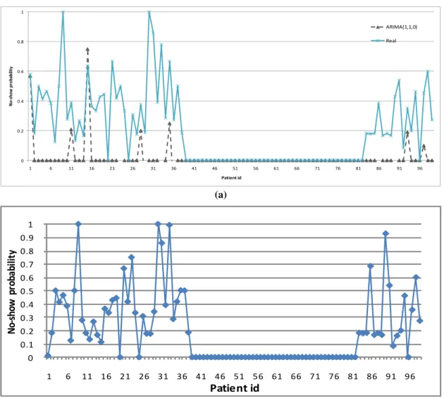
probability of no-show, (b) Absolute difference of estimated and real no-show probability Finally, Figure 6(a) shows the results from ARIMA (1,1,0) model which is one of the individual based methods. As can be seen for a large portion of patients that have real no-show
rate of larger than zero ARIMA can barely follow the real pattern. This can also be checked in Figure 6 (b) which has several differences greater than 0.5 and a few differences equal to 1.
0 0.2 0.4 0.6 0.8 1 1 6 11 16 21 26 31 36 41 46 51 56 61 66 71 76 81 86 91 96 No ‐ sh o w pr o ba bilit y Patient id ARIMA(1,1,0) Real (a) 0 0.1 0.2 0.3 0.4 0.5 0.6 0.7 0.8 0.9 1 1 6 11 16 21 26 31 36 41 46 51 56 61 66 71 76 81 86 91 96 No ‐ sh ow pr ob ab ilit y Patient id (b)
Figure 6: ARIMA (1,1,0) performance over patients: (a) estimated versus real probability of no-show, (b) Absolute difference of estimated and real no-show probability
2.2.2.2. Patient wise Analysis
Here the comparing methods discussed in previous Sections are studied based on a patient wise analysis. For this purpose, out of 99, 50 patients are randomly chosen and used for training, 20 are randomly selected for validation and the 29 are used for testing. Figure 7 illustrate the results which is similar to time wise analysis of the comparing methods.
Proposed ARMA (1,0,1) Box
Smoothing Decision Tree
Logistic
regression ARMA (2,0,2) Rule‐based
MSE 0.013 0.027 0.03 0.033 0.052 0.053 0.059 0.00 0.02 0.03 0.05 0.06 0.08
Figure 7: Mean squared error (MSE) of different methods used for comparison comparing methods
The results from Figures 2 to 7 clearly show the capability of the proposed model in estimating probability of non-attendance for both current and new patients of a health care system.
2.2.2.3. Discussion
In this Section, up to this point, a probabilistic model based on logistic regression and Bayesian inference has been developed to estimate the patients’ no-show probability in real-time. Also, the effects of appointment date and clinic on the proposed method have been modeled. Next, based on a dataset from a Veteran Affair medical center, the effectiveness of the approach has been evaluated. Our approach is computationally effective and easy to implement. Unlike population based methods, it takes into account the individual behavior of patients. Also, in contrast to individual based methods, it can put together consolidated information from the entire data to provide reliable initial estimates. In the next Section, the proposed method is extended to consider other types of disturbances.
2.3. Generalization of the Proposed Algorithm for No-Show and Cancellation
Prediction
Algorithm 2 illustrates the pseudo code of the proposed algorithm for estimating two types of disruptions probabilities: no-show and cancellation. Similar to Algorithm 1, algorithm 2 consists of the following three main components:
1. Initial no-show and cancellation probabilities estimation 2. Bayesian update of the no-show and cancellation estimates 3. Weight optimization
Algorithm 2: No-show and Cancellation Prediction Algorithm Input: Input data , , Threshold parameter
Output: Estimated no-show and cancellation probabilities ̂ , Dirichlet distribution posterior parameters , Multinomial logistic regression estimated parameters
Procedure:
1 /* Logistic regression*/
2 Calculate MLE of Equation (1-5) parameter
3 ̂ 1,2,3| , 4 ̂ 5 /*Weight optimization*/ 6 ̂ ∑ 1
7 Until Equation (2-1) improvement do
8 set a value for the vector of appointments weights
9 /*Bayesian update */ 10 , , 11 ̂ ∑ 12 ̂ , … , ̂ 13 ∑ 14 ∑ ′ 15 16 17 , , 18 Return ̂
In the first component, based on the training dataset consisting individuals’ personal information , (such as gender, marital status, etc.) and their sequence of appointment information (e.g. previous attendance records )), a multinomial logistic regression model
, is formulated (line 2). Then, using logistic regression, an initial estimate of no-show, cancellation and show-up probabilities are calculated, given by ̂ 1,2,3| (line 3). As discussed in Section 1.1.2, Logistic regression bundles the information of the complete population together and finds a reliable initial estimate of no-show ( ̂ .
In the second component, which is interlaced with the third component, the initial estimate is used in a Bayesian update procedure to find the posterior no-show, cancellation and show-up probabilities of each person. For this purpose, ̂ is transformed into prior parameters of a Dirichlet distribution as shown in line 4. Next, using the attendance record of each person the posterior parameters and posterior probability of attendance ̂ is calculated (lines 10 and 11). As discussed in Section 1.1.3, the reason for applying the Bayesian update procedure to the output of logistic regression is that, typically regression models cannot consider individual patients behavior. Also, updating regression parameters based on new data records is both difficult and only marginally effective (especially when the model is already constructed on a huge dataset) in comparison to Bayesian update.
In the third component, appointments are weighted based on a subset of factors W=
, … , (line 8) to increase the model performance in estimating the real probability of
no-show. An optimization procedure is used for finding the optimal value of the weights. The objective function of the model is to minimize the difference between the empirical and estimated probabilities of no-show, cancellation and show-up as follows:
(
)
ω α ,.., 1 1 0 : . max 0 , , = ≤ ≤ > = − − − q w T S F F p value p q p n p test F paired (2-4)Where , … , are the weights to be optimized and is the p-value of a one-sided statistical hypothesis testing of the paired estimated p using the model and estimated p
using the attendance records:
⎩ ⎨ ⎧ ≠ = al D Model D al D Model D p p H p p H Re 1 Re 0 : : ( 2-5)
It should be noted that MSE can also be used as the objective function. However, statistic which is used above not only contains MSE information in itself (both in the statistics and
MSE estimate the deviation of a variable from its nominal value) (line 14), but also has a statistical distribution which makes it a better choice for our optimization model.
In Equation (2-4), , , is the percentage of points or value of F random variable with K
and n-K degrees of freedom such that the probability that , exceeds this value is , and , where is calculated through lines 11 -15. ̂ in line 11, shows the real rate of no-show, cancellation and showing up for person calculated as
̂ ∑ with as a multinomial (random) variable representing the records of attendance of type for patient i and appointment j. Here, is the index of first appointment in the validation dataset which is discussed shortly, and is the index of last appointments in the validation dataset for patient i. Also, ̂ ∑ is the estimated probability of disruption of type calculated based on weighted appointments in validation dataset using the proposed model.
The optimization procedure is as follows: at every iteration, a vector of weights is assigned to the appointments in validation dataset (line 8). The weighted appointments are then plugged into the Bayesian update mechanism for estimating the probability of no-show (lines 10 and 11). Next, the estimates of the proposed model and real attendance records are compared by forming a -statistic (lines 12 to 16) and the p-value of the paired -test (line 17) which shows the goodness of the assigned weights, is used for improving the initial set of weights (line 7) . This procedure continues until no improvement is observed. Then, the ̂ of the iteration resulted in the best value of objective function is used as the no-show estimate (line 18).
2.4. Experimental Results
For the purpose of evaluation, the performance of the proposed method is evaluated along with different population-based and individual-based algorithms on the extended version of the dataset used in the previous Section which includes 1,543 patient records with the following appointment information: (1) sex, (2) date of birth (DOB), (3) marital status, (4) medical service coverage, (4) address (zip code), (5) clinic and (6) prior attendance record in the hospital. 3-fold cross-validation with approximately 500 records each for training, validation and testing is considered for the evaluation.
We will first discuss the preprocessing of the data and then provide a stylized example for one sample patient record to illustrate how the model works. Finally, the result of applying the model on the dataset is discussed based on two types of analysis: (i) time-wise analysis and (ii) patient-wise analysis.
2.4.1. Data Preprocessing
As discussed in Section 2.2.1, before applying the proposed model to the dataset, it should be preprocessed (see Section 2.2.1 for more information). Table 6 shows the result of clustering the clinics based on their probability of no-show, cancellation and show-up using GMM. This Table is an extension to the Figure 1(b) in Section 2.2.1 . In the Section 2.2.1 the clinics are grouped based only one type of disruption, namely no-show rate. However, here they are clustered based on two types of disturbances, namely no-show and cancellation.
Table 6: The result of clustering the clinics based on their no-show, cancellation and show-up probabilities Cluster Attribute Parameter 0 1 2 3 4 No-show 0.0015 0.3488 0.2167 1.0000 0.1377 0.0114 0.1557 0.2692 0.3085 0.1331 Cancellation 0.0011 0.0540 0.7833 0.0000 0.3276 0.0088 0.0733 0.2692 0.1968 0.1251 Show-up 0.9974 0.5972 0.0000 0.0000 0.5346 0.0142 0.1523 0.0031 0.3372 0.1465
Again, like previous Section, (1) appointment recency, (2) appointment preceding non-work days (Saturday, Sunday, and holidays), and (3) clinic cluster, are considered as weighting factors ( , , , which are arranged in the data structure illustrated in Table 7. Table 7 also shows the optimal values of the weights used in Section 2.4.2 analysis.
Table 7: Data structure and optimal value of the weighting factors A n al ysis Val idat ion s et Appointment Recency Preceding
non-workday Clinic Cluster
<1 w k . <1 mon . <3 mon . 6< mon . > 6 mo n. N o t-b efo re ho li d a y Before ho li d a y Extremel y import a n t Highly import a n t Moderately import a n t Low import a n t No t import a n t tim e w is e 1 1 1 1 0.75 0.5 1 0.90 1 1 0.9 0.81 0.62. 2 1 0.97 0.96 0.82 0.67 1 0.98 1 1 0.84 0.73 0.71 3 1 1 1 0.87 0.78 1 0.97 1 0.87 0.81 0.80 0.75 Patient wi se 1 1 2 1 0.99 0.75 0.61 0.58 1 0.89 1 1 0.82 0.73 0.70 1 1 1 0.94 0.85 0.77 0.69 1 0.81 0.69 0.66 3 1 1 0.89 0.81 0.51 1 1 1 1 0.89 0.69 0.55
2.4.2. Applying the Proposed Model to a Sample Patient
The Section explains different steps of the proposed approach using a simple case study on a randomly selected patient. The patient was male, born on 02/5/1978, never married, degree of medical service coverage less than 5% with zip code 48235. Table 8 shows his appointment information as patterns of show/no-show from 10/13/2009 to 12/31/2009 (training data). Note that no-shows are represented by 1 while cancellation and show-ups are represented by 2 and 3 respectively.
Table 8: No-show, cancellation and show-up record of a sample patient
Appointment
No. Appointment date
Clinic cluster Weight Attendance record Preceding non-workday Recency Clinic cluster 1 10/1/2009 0 1 0.5 0.9 3 2 10/8/2009 0 1 0.5 0.9 1 3 10/9/2009 0 0.9 0.5 0.9 2 4 10/13/2009 2 1 0.5 1 3 5 10/13/2009 2 1 0.5 1 3 6 10/13/2009 2 1 0.5 1 3 7 10/15/2009 0 1 0.5 0.9 3 8 10/15/2009 2 1 0.5 1 3 9 10/19/2009 2 1 0.5 1 1 10 10/19/2009 2 1 0.5 1 1 11 10/19/2009 0 1 0.5 0.9 1 12 10/22/2009 2 1 0.5 1 3 13 11/6/2009 2 0.9 0.5 1 3 14 11/6/2009 0 0.9 0.5 0.9 3 15 12/3/2009 2 1 0.5 1 3 16 12/18/2009 2 0.9 0.5 1 3
Using the patient’s personal and appointment information as well as his previous attendance record, the parameters of the fitted multinomial logistic regression model are computed as shown in Table 9 (since we are modeling a categorical variable with three levels, namely no-show, cancellation and show-up, two sets of regression parameters are estimated (See Equation 1-5) .
Table 9: A sample multiple logistic regression model fitted to the dataset
Se x DO B
Marri age status
Me di cal se rvi ce
cove rage Zi p code
C l i ni c cl uste r Re ce ncy C l ose ne ss to non-workday C onstant 106.605 -2.994 0.000 -0.314 -0.063 -0.002 -0.733 1.175 -0.388 168.919 -4.015 0.000 -0.234 -0.058 -0.003 -0.973 0.638 1.122
Based on the estimated coefficient the probability of no-show, cancellation and show-up for the first appointment in the testing dataset (2/1/2010) is estimated as (0,52525, 0.050374, 0.424376). This estimate is used for building the prior Dirichlet distribution with same parameters. Table 10 illustrates the updated parameters of Dirichlet distribution after each appointment.
Table 10: Bayesian update of Dirichlet distribution parameters Appo intment No. Appo intment da te C lin ic catego ry Weight Att end a n ce record Estimate Probability No -S h o w Cancell a ti on S h ow -up Preceding no n -w o rk da y Recency C linic cluster 0.5253 0.0504 0.4244 18 2/1/2010 2 1 0.75 1 1 0.7626 0.0252 0.2122 19 2/5/2010 2 0.9 0.75 1 3 0.3051 0.0101 0.6849 20 2/5/2010 2 0.9 0.75 1 1 0.4209 0.0084 0.5707 21 2/5/2010 0 0.9 0.75 1 3 0.2806 0.0056 0.7138 22 2/9/2010 2 1 0.75 1 1 0.3525 0.0050 0.6424 23 2/9/2010 2 1 0.75 1 1 0.4114 0.0046 0.5840 24 2/9/2010 2 1 0.75 1 1 0.4604 0.0042 0.5354 25 2/10/2010 2 1 0.75 1 1 0.5019 0.0039 0.4942 26 2/17/2010 2 1 0.75 1 3 0.4078 0.0031 0.5890 27 3/15/2010 2 1 0.75 1 3 0.3434 0.0027 0.6539
Figure 8 (a) illustrates the changes in the estimated probabilities of no-show, cancellation and show-up after each new record of attendance (solid lines) plus the estimated trend (using order three polynomials) of each type (dashed lines). Figure 8 (a) shows how the Bayesian update reacts quickly to each new data record, which means that the procedure can rapidly converge to the real distribution of no-show. Figure 8 (b) compares the prior and posterior distributions of this patient attendance probability before and after applying testing data. It is easy to follow the movement of the probability density function to the right and upper edges of the simplex (indicated by the arrows) which can be interpreted as decreasing the probability of cancellation significantly.
(a)
(b) (c)
Figure 8: Applying the proposed model for a sample patient: (a) changing parameters during Bayesian update (b) prior distribution (c) posterior distribution
2.4.2.1. Time wise Analysis
This Section study the performance of the proposed model along with representatives from population-based and individual-based algorithms based on time-wise analysis. The training, validation and testing data are constructed as follows: appointments that occurred before 11/23/2009 have been used for training; appointments between 11/23/2009 and 2/1/2010 have been chosen for validation, and finally, appointments after 2/1/2010 have been considered for
0.0 0.1 0.2 0.3 0.4 0.5 0.6 0.7 1 2 3 4 5 6 7 8 9 10 11 Prob ab ility Appointment No. No‐show Cancelation
Show‐up Poly. (No‐show)
Poly. (Cancelation) Poly. (Show‐up)
0 0.2 0.4 0.6 0.8 1 0 0.5 1 0 50 100 150 200 x2 x1 f( x 1 ,x 2, 1-x 1 -x 2) 0 0.2 0.4 0.6 0.8 1 0 0.5 1 0 200 400 600 800 1000 x2 x1 f( x 1 ,x 2, 1-x 1 -x 2)
testing. The main reason for selecting the above dates is to have approximately equal number of data records each in the training, validation and testing datasets.
The methods used in our comparison are the following: locally weighted scatter plot (LOESS), Savitzky-Golay, Box, and Gaussian which are used as smoothing techniques (Simonoff [1996]), decision tree (DT), multiple logistic regression (with same predictors as used in the proposed model regression part) and pure multinomial Bayesian update, Bayesian Net, Multilayer Perceptron Neural Net (MLP) and a boosting algorithm. For setting the parameters of the comparison methods, the size of the moving window for Box smoothing was varied over the range of 1 to 7 and the optimal size (5) was considered for the comparisons. The standard deviation parameter of Gaussian distribution is experimented over 0.2 to 1; while 0.65 (the optimal value) was used. J48 was used for building the decision tree and ADABOOST PART [Viola and Jones 2002] algorithm is used for boosting method. For the pure Bayesian updating the Jeffery’s prior 0.33, 0.33, 0.33 is considered as the prior [Bolstad 2007]. For the multinomial logistic regression and smoothing methods the whole data set is used for building the model.
Figure 9 illustrates the MSE of the different methods used for comparisons. Based on the MSE measure, the proposed model outperforms other methods, while the rule-based method has the worst performance. As can be seen from the results, in general, individual-based methods outperform population-based methods, while bundling these methods together (as in our proposed method) significantly improves the overall performance.
Proposed method Pure Bayesian Pure Logistic Regression LOESS Smoothing Guassian Smoothing SGOLAY Smoothing Box Smoothing ADABOOST MLP Bayesian Net DT MSE 0.06551717 0.10134571 0.13662156 0.20534544 0.21575823 0.23151254 0.3308683 0.91445237 1.19313027 1.47764096 1.53726507 0 0.2 0.4 0.6 0.8 1 1.2 1.4 1.6 1.8
Figure 9: Mean Squared Error (MSE) of the studied methods for time-wise analysis Figures 10-12 compare the empirical and estimated probability of no-show and cancellation for the methods over different patients (the performance of other methods along with the source code is available upon request). As shown in Figure 12, the proposed approach often predicts the real pattern correctly with considerable small variance.
0 0.2 0.4 0.6 0.8 1 1.2 1 6 11 16 21 26 31 36 41 46 51 56 61 66 71 76 81 86 91 96 P ro b a b il it y Patient Id
No show (Real) Cancelation (Real) No show (Proposed) Cancelation (Proposed)
Figure 10: The performance of the proposed approach over different patients: estimated versus empirical probability of no-show and cancellation
Figure 11 illustrates the estimates from multinomial logistic regression, a population-based method. The estimates tend to have small fluctuations around an approximately fixed mean, though in general it somehow resembles the true pattern of the real no-show and cancellation. In addition, the difference between the estimated and real series significantly increases for patients with tendency of not cancelling their appointments (those could be either patients with good records of showing-up or those with high rate of no-show). Such result clearly shows that the regression models may not fully capture the difference among patients’ personal behaviors.
0 0.2 0.4 0.6 0.8 1 1.2 1 6 11 16 21 26 31 36 41 46 51 56 61 66 71 76 81 86 91 96 P ro b ab ilit y Patient id
Simple Average No show (Real) Simple Average Cancelation (Real) Pure Regression No show (Logistic) Pure Regression Cancelation (Logistic)
Figure 11: The performance of pure multinomial logistic regression over different patients: estimated versus empirical probability of no-show and cancellation
Finally, Figure 12 shows the results from pure Bayesian update method, which is a popular individual-based method. It can be seen that pure Bayesian update can basically detect the fluctuations in the real series correctly; however the estimates are far from the real ones in considerable number of cases. Further analysis revealed that such cases contain few number of attendance records which means that the pure Bayesian parameters update could not neutralize the effect of prior especially if that is far from the real case.
0 0.2 0.4 0.6 0.8 1 1.2 1 6 11 16 21 26 31 36 41 46 51 56 61 66 71 76 81 86 91 96 Pr ob ab ili ty Patient id
No show (Real) Cancelation (Real) No show (Bayesian) Cancelation (Bayesian)
Figure 12: The performance of pure Bayesian updating method over different patients: estimated versus empirical probability of no-show and cancellation
2.4.2.2. Patient wise Analysis
Here the proposed method is compared to some other methods in the literature using patient-wise analysis. For this purpose, out of 99 patients in the database, using 3-fold cross-validation, 33 patients were randomly chosen for training, validation and testing. Figures 13-16 illustrate MSE and pairwise comparison of the empirical and estimated no-show and cancellation probabilities of the comparing methods which reveals similar results to the time-wise analysis discussed in the previous Section.
Proposed Pure
Bayesian SGOLAY LOWESS Bayesian Net Logistic
Regression ADABOOST DT MLP Guassian Box
MSE 0.001840403 0.01625156 0.049004329 0.097390678 0.14107536 0.14220441 0.14830201 0.16112196 0.17123044 2.075866983 3.070707071 0 0.5 1 1.5 2 2.5 3
Figure 13: Mean Squared Error (MSE) of the studied methods for patient-wise analysis
0 0.2 0.4 0.6 0.8 1 1.2 1 2 3 4 5 6 7 8 9 10 11 12 13 14 15 16 17 18 19 20 21 22 23 24 25 26 27 28 29 30 31 32 33 34 P ro b a b il it y Patient id
Empirical No‐show Empirical Cancelation Estimated No‐show Estimated Cancelation
Figure 14: The performance of the proposed approach over different patients: estimated versus empirical probability of no-show and cancellation
0 0.2 0.4 0.6 0.8 1 1.2 1 2 3 4 5 6 7 8 9 10 11 12 13 14 15 16 17 18 19 20 21 22 23 24 25 26 27 28 29 30 31 32 33 34 Pr ob ab ili ty Patient id
Estimated No‐show Estimated Cancellation Emprical No‐show Emprical Cancelation Figure 15: The performance of pure multinomial logistic regression over different patients: estimated versus empirical probability of no-show and cancellation
0 0.2 0.4 0.6 0.8 1 1.2 1 2 3 4 5 6 7 8 9 10 11 12 13 14 15 16 17 18 19 20 21 22 23 24 25 26 27 28 29 30 31 32 33 34 Estimated No‐show Estimated Cancelation Emprical No‐show Emprical Cancelation
Figure 16: The performance of pure Bayesian updating method over different patients: estimated versus empirical probability of no-show and cancellation
The results from Figures 13-16 clearly show the capability of the proposed model in estimating probability of disruptions for both current and hypothetical patients of a health care system.
2.4.2.3. Discussion
In this Section, the probabilistic model in the previous Section has been extended to estimate the individuals’ probabilities of no-show, cancellation and showing up in real-time. Also based
on real-world patient data collected from a Veterans Affairs medical hospital, the effectiveness of the approach was evaluated. The result of the proposed method can be used to develop more effective appointment scheduling systems and more precise overbooking strategies to reduce the negative effect of no-shows and fill in appointment slots while maintaining short waiting times which is discussed in the next chapter.