Modeling Correlation in Vehicle Routing Problems with Makespan Objectives and Stochastic Travel Times

WORKING PAPER SERIES

Modeling Correlation in Vehicle Routing Problems

with Makespan Objectives and Stochastic Travel Times

Iurii Bakach/Ann Melissa Campbell/Jan Fabian Ehmke/Timothy L. Urban

Impressum (§ 5 TMG

)

Otto-von-Guericke-Universität Magdeburg Fakultät für Wirtschaftswissenschaft DFS Dekan

Verantwortlich für diese Ausgabe:

Otto-von-Guericke-Universität Magdeburg Fakultät für Wirtschaftswissenschaft Postfach 4120 39016 Magdeburg Germany http://www.Gww.PWHVEF/femm

Modeling Correlation in Vehicle Routing Problems

with Makespan Objectives

and Stochastic Travel Times

Iurii Bakach

, Ann Melissa Campbell

, Jan Fabian Ehmke

, and Timothy

L. Urban

1

Mathematics Department, The University of Iowa, 2 West Washington Street, Iowa City, Iowa 52242, US, [email protected]

2_{Management Sciences Department, Tippie College of Business, University of Iowa, 21 E Market St, Iowa}

City, Iowa 52242, US, [email protected]

3_{Management Science Group, Otto-von-Guericke Universit¨at Magdeburg, Universit¨atsplatz 2, 39016}

Magdeburg, Germany, [email protected], phone +49-391-6758225, fax +49-391-67658225,

corresponding author

4_{Collins College of Business, School of Finance, Operations Management and International Business, The}

University of Tulsa, 800 South Tucker Drive Tulsa, Oklahoma 74104, US, [email protected]

May 2, 2018

Abstract

The majority of stochastic vehicle routing models consider travel times to be in-dependent. However, in reality, travel times are often stochastic and correlated, such as in urban areas. We examine a vehicle routing problem with a makespan objective incorporating both stochastic and correlated travel times. We develop an approach based on extreme-value theory to estimate the expected makespan (and standard de-viation) and embed this within a routing heuristic. We present results that demonstrate the impact of different correlation patterns and levels of correlation on route planning.

1

Introduction

Much of the existing research on stochastic routing problems assumes that the travel times on arcs in the network are independent of one another. Empirical studies, though, show that correlation is evident in many locations. Park and Rilett (1999) analyze data obtained from the Houston freeway system and found considerable correlation between some of the arcs of the freeway, with correlation coefficients as high as 0.75. Travel time correlation was also identified in truck routing data from Sydney, Australia (Figliozzi et al., 2007). He et al. (2002) simulated the Irvine, California corridor network using GPS-based vehi-cle records and found statistically-significant correlation in travel times, with both positive and negative correlation coefficients. Guo (2006) suggests arc travel times may be corre-lated due to weather effects and secondary incidents and their impact on the behavior of roadway users, and notes that assuming independent travel times can lead to biased so-lutions. Eliasson (2007) also found positive and negative correlations using an automatic travel time measurement system in Stockholm. Jenelius (2012) notes that poor weather conditions can affect travel times on several arcs. Nicholson (2015) suggests that negative correlation can occur when a bottleneck in one location results in increased speeds on the downstream locations. Fan et al. (2005) note that travel time correlation might also be an important aspect to consider in routing emergency vehicles through networks after a natural disaster.

In combining correlation with stochastic travel times, the sum of the expected travel times is not directly impacted by the correlation of the travel times (Rostami et al., 2017), but the expected makespan of the routes is. The makespan is the cost, typically time or distance, to complete the longest route. Bertazzi et al. (2015) note that this is a better objective in a number of situations, such as driver workload balance, computer networks, and disaster relief efforts. In terms of workload balance, the makespan represents the completion time of the longest driver route. If one driver has a much longer route than other drivers, this can promote job dissatisfaction and impact driver retention, which is a known business challenge (Ulmer et al., 2017). In disaster relief, the makespan reflects the time when all destinations affected by the disaster have been served.

The purpose of our research is to investigate a makespan routing problem with stochas-tic and correlated travel times. A makespan objective with stochasstochas-tic and correlated travel times requires the use of a complex objective function evaluation or the use of extensive simulations. In this paper, we present a way to approximate the expected makespan and the standard deviation of makespan utilizing extreme-value theory. We evaluate the quality of these approximations and show them to be comparable with simulation with a drastically reduced computation time. We then embed these approximations within routing heuristics to solve for the routes that minimize the expected makespan. We also examine minimizing

the makespan plus one standard devation to capture the potential variability. For example, when considering the workload balance example, a driver who has the longest expected route length will likely be dissatisfied if this route also has high variation in travel time. The addition of a measure of variability to the objective has been considered in the study of shortest path problems with correlation (e.g. Zockaie et al. (2014)) and in min-sum stochastic routing problems (e.g. Rostami et al. (2017)). We perform computational ex-periments for both objectives to help develop an understanding of how correlation changes the routes. The datasets we use are based on Solomon instances with the addition of dif-ferent arc correlation patterns based on ideas from literature on correlation.

A brief review of related literature is presented in the next section. In Section 3, we discuss how correlation can impact the expected makespan. In Section 4, we describe a procedure using extreme-value theory to approximate the makespan and its standard deviation. We evaluate the accuracy of these approximations through simulation. These approximations are then incorporated into a vehicle-routing algorithm in Section 5, and computational experiments are presented in Section 6. Finally, we conclude the paper and present suggestions for future research in Section 7.

2

Literature Review

This review of related routing problems consists of three parts. First, we present a review of the research on min-max objectives for both node-routing and arc-routing problems. Then, stochastic routing problems are discussed, focusing on problems with random travel times. Finally, path finding and routing problems that incorporate travel time correlation are reviewed.

2.1

The Min-Max Routing Problem

Frederickson et al. (1976) were the first to consider min-max, multiple-route routing prob-lems. They show that the multiple traveling salesmen problem (kTSP), the multiple Chi-nese postman problem (kCPP), and the multiple stacker-crane problem (kSCP) are NP-complete, and they develop heuristics using previously-developed methods from the re-spective minimum-cost, single-route heuristics. Arkin et al. (2006) also consider several node-routing and arc-routing problems and provide approximation algorithms for each.

Most of the recent focus on the multiple traveling salesmen problem has been on de-veloping efficient solution methodologies using metaheuristics. This research includes the use of tabu search (Franc¸a et al., 1995), neural networks (Modares et al., 1999), genetic algorithms (Carter and Ragsdale, 2006; Singh and Baghel, 2009), and ant colony opti-mization (Liu et al., 2009). An extension to this problem is the location-allocation kTSP,

where the location of the depot is found in addition to the allocation of customers to routes (Averbakh and Berman, 1997; Nagamochi and Okada, 2004; Xu et al., 2013).

The vehicle routing problem is a generalization of the multiple traveling salesmen problem by including capacities on the vehicles (CVRP), time windows on deliveries to customers (VRPTW), etc. Golden et al. (1997) present an adaptive-memory heuristic for the kTSP and the CVRP with and without the multiple use of vehicles. Modares et al. (1999) suggest the use of neural networks for the CVRP, and Ren (2011) propose a hybrid genetic algorithm. A branch-and-cut search has been developed by Applegate et al. (2002) to optimally solve a 120-customer, 4-vehicle problem using distributed processing. Campbell et al. (2008) note that the min-max VRP is applicable in the routing of critical supplies for disaster relief; they also formulate a second objective in which the average time to each customer is minimized. Bertazzi et al. (2015) conduct a worst-case analysis comparing the min-max objective and the traditional min-sum objective and find that the length of the longest route when solving the min-sum VRP can be as much asktimes the longest route in the min-max problem, wherek is the number of vehicles, motivating the need to design efficient heuristics for the min-max problem.

Recent research has analyzed several variants of the min-max vehicle-routing problem. Carlsson et al. (2009), Narasimha et al. (2013), and Wang et al. (2015) consider the min-max VRP with multiple depots, in which a vehicle must start and end at the same depot. Xu et al. (2010) investigate the VRP in which a depot must be selected from a given set, and Valle et al. (2011) consider the VRP in which not all customers need to be visited by a vehicle as long as they are close enough to another customer that is on the route. Yakıcı and Karasakal (2013) extend the problem to account for split deliveries and heterogeneous demand.

Relatively little research has been identified on min-max, multiple-route arc-routing problems since the articles of Frederickson et al. (1976) and Arkin et al. (2006) men-tioned above (see Benavent et al. (2014) for a review). Lacomme et al. (2004) develop memetic algorithms for the capacitated arc-routing problem. Ahr and Reinelt (2006) solve the kCPP using tabu search. Benavent et al. (2009) and Benavent et al. (2010) investigate the multiple windy rural postman problem, developing a branch-and-cut method as well as a multi-start/local-search heuristic; Akbari and Salman (2017) propose a heuristic for this problem based on an MIP-relaxation and a local-search algorithm. Willemse and Jou-bert (2012) discuss the application of the kCPP to the patrolling of an estate by security guards; they provide a tabu-search heuristic to solve the kCPP as well as the multiple rural postman problem when a subset of the network is patrolled.

2.2

Routing Problems with Stochastic Travel Times

Most of the stochastic routing research literature is concerned with stochastic customers (each customer has some probability of realizing demand) and/or demands (the demands are random variables); very little considers stochastic travel times for either node-routing problems (Cordeau et al., 2007) or arc-routing problems (Wøhlk, 2008). Shortest path problems have incorporated stochastic times – even with correlations between times – but are only concerned with finding the shortest time between two vertices of a network (e.g., Burton (1993)) or a set of non-dominant paths (Ji et al. (2011)). Various single-route rout-ing problems have also incorporated stochastic travel times, such as the travelrout-ing salesman problem (beginning with Leip¨al¨a (1978) and Kao (1978)), and the Chinese postman prob-lem (Tan et al., 2005). However, the only multiple-route probprob-lems found that incorporate stochastic travel times are in the context of the vehicle routing problem (VRP, recent re-views of stochastic vehicle routing are provided by Ritzinger et al. (2016) and Gendreau et al. (2016)).

Cook and Russell (1978) use simulation to evaluate the quality of deterministically-generated routes on the VRP with stochastic travel times. Laporte et al. (1992) were the first to incorporate stochastic travel times as part of a VRP model; they present two versions of the problem: (i) chance-constrained programming and (ii) stochastic program-ming with recourse. They use a branch-and-cut algorithm to solve problems with up to 20 vehicles and travel times that can take on a value from as many as five discrete states. Lam-bert et al. (1993) develop a model specific to a particular banking context in which travel time is based on a given probability the route is congested. Kenyon and Morton (2003) consider two models with different objective functions: (i) minimizing the expected time that all vehicles will return to the depot and (ii) maximizing the probability of complet-ing the routes by a given deadline. They develop a branch-and-cut approach to solve the problem when the cardinality of the sample space is small and embed a sampling-based procedure for larger sample spaces or continuous random parameters.

The vehicle routing problem with time windows (VRPTW) and stochastic travel times has recently been investigated using genetic algorithms (Ando and Taniguchi, 2006) and tabu search (Russell and Urban (2008); Li et al. (2010); Tas¸ et al. (2013); Zhang et al. (2013)); these models include a penalty in the objective function and/or a constraint lim-iting the probability of not meeting the time-window constraint. Tas¸ et al. (2014) propose an exact solution approach based on column generation and a branch-and-price method. Lecluyse et al. (2009) also consider the VRPTW, but include the standard deviation of the travel time as part of the objective function. Based on extreme-value theory, Ehmke et al. (2015) approximate chance constraints for the VRPTW and adapt a tabu-search algo-rithm to ensure a certain level of arriving within customer time windows. Adulyasak and

Jaillet (2015) consider the VRP with deadlines in both the stochastic (known probability distribution) and robust (unknown, but belonging to a family of distributions) cases. Tas¸ et al. (2014) consider time dependency in the modeling of stochastic travel times. Time dependency has also been considered in modeling the dial-a-ride problem with scheduled pickup-drop-off times by Fu (2002), Xiang et al. (2008), and Schilde et al. (2014). Related problems in which the customer service times are stochastic were considered by Sungur et al. (2010), Lei et al. (2012), and Errico et al. (2016). The only min-max routing problem identified in the literature that incorporates stochastic travel times is Kenyon and Morton (2003), and they note that for large problems “Monte Carlo sampling may be the only vi-able option.” And while they note that the travel times may be dependent in their models, they do not explicitly evaluate the effect of correlated travel times.

2.3

Routing Problems with Correlation

We were able to identify several papers that consider stochastic travel times and correlation for path finding or vehicle routing.

Zockaie et al. (2013) consider a shortest path problem with on time arrival probabil-ity (SPOTAR) between an origin-destination pair in a network with random travel times. Their motivation is to check the effect of the correlation on reliable path finding. To quan-tify the impact of correlation, a two-stage algorithm based on Monte Carlo simulations is presented. The authors investigate only spatial correlation between neighboring adjacent arcs. One of the conclusions is that correlation has a complex impact on route choice.

In Zockaie et al. (2014), the minimum path travel time budget problem (MPTTB) on a Chicago-based network is considered. The travel time budget is addressed by a reliability index defined as a linear combination of mean travel time and standard deviation. Two so-lution methods are implemented and compared: an outer approximation method based on a cutting-plane algorithm and Monte Carlo simulations. Only spatial correlation between neighboring adjacent arcs is investigated.

Zockaie et al. (2016) extend their Monte Carlo simulation approach, developed in Zockaie et al. (2013) and Zockaie et al. (2014) for SPOTAR and MTTBP, for stochastic time varying networks with spatial and temporal travel time correlations. The developed method considers arc travel time correlations by drawing random numbers from a joint arc travel time distribution instead of treating arcs independently. For temporal correlation, consecutive time intervals are assumed to be correlated, and for spatial correlation, instead of considering a correlation only between two neighboring arcs, the authors consider it between three neighboring arcs. We allow for any arcs in the network to be correlated, but we do not explicitly consider different time periods.

matrix for spatially and temporally correlated travel times. Given a high dimensionality of a joint spatial-temporal correlation matrix, their approach provides an intuitive and logical method to create a valid correlation matrix. They use a heuristic test to identify whether there are enough simulation scenarios for their numerical results to be valid.

Jiang and Mahmassani (2014) consider a time-dependent vehicle routing problem with time windows in congested urban environments. They use simulation to retrieve informa-tion on the dynamics of traffic within the road network. Their soluinforma-tion approach is based on a two-phase set-partitioning-based heuristic. It is applied to two real-world networks, Fort Worth and Chicago, and time-dependent travel times were obtained under various in-cidents. Numerical results show that different events may significantly affect the quality of the solution. For instance, weather incidents such as heavy snow fall increased the total time of the route plan by more than 45%, and not considering the incidents leads to mul-tiple violations of customer time windows. We use their observations about disruptions in one of our tested correlation patterns.

Rostami et al. (2017) investigate a capacitated vehicle routing problem with correlated stochastic travel times. The objective function is to maximize the travel time reliability, which is represented as a linear combination of travel time and its variance. They model the problem as binary quadratic program and propose two alternative set partitioning refor-mulations. They solve their problem for two different types of correlation: correlation only between adjacent arcs and correlation between all arcs. Computational results based on well-known Solomon datasets show that travel time variance could be reduced up to 70% for some instances. We mimic their use of Solomon datasets but use different correlation matrices and a makespan objective.

3

Analyzing the Effect of Correlation on Makespan

The model under consideration is an extension of the mixed general routing problem (MGRP) presented by Corber´an et al. (2005). LetG= (V, E, A)be a strongly-connected mixed graph with vertex setV, edge setE, and arc setA. Multiple vehicles are available to serve a subsetV_R ⊆V of required vertices. We assume the time (cost) to traverse each arc of the network,L∈E∪A, is a random variable; these times are not required to be in-dependent nor identically distributed (non-IID). The objective is to minimize the expected value of the makespan (min-mean-max) or the expected value plus some multiple of the standard deviation. Our focus is on the travel times so, as long as the time to complete each route can be determined by the sum of the times to traverse a set of arcs and vertices of the network, our analysis should be applicable.

3.1

Effect of Arc Correlation on Route Correlation

It is well known how correlation affects the variance of a combination of variables. The benefits of risk pooling (e.g., for portfolio diversification, supply chain management, insur-ance) decrease as the correlation between the variables becomes more positive. However, with our min-mean-max objective, it is not straightforward what the impact of correlation will be, so we need to identify the correlation between routes as well as the expected value and variance of route times.

Let the travel time on any arc follow an arbitrary distribution with a mean ofμ_i and a variance ofσ2_i. These travel times need not be independent; the correlation of the time to travel arciand arc kisρ_ik, hence a covariance ofσ_ik = ρ_ikσ_iσ_k. A route, then, consists of traveling from the depot, over a set of arcs and back to the depot. The travel time for the entire route will tend toward – but not necessarily achieve – a normal distribution due to the Central Limit Theorem, with a mean of E(Y) = _i∈Rμ_i and a variance of V ar(Y) =_i∈Rk∈Rσik, whereσii=σi2andρii= 1. Since the individual travel times between arcs are correlated, the route times will also be correlated.

The correlation of two linear combinations of variables can be determined as follows (see, e.g., Johnson and Wichern (2007)). LetX1 andX2 be two random vectors of size n and m, respectively (hence, we index i and k from 1 to n for X₁ as well as j and l fromn+ 1 ton+mfor X2), with variance/covariance matrices of V11 andV22, respec-tively. The covariances between pairs of variables from different sets (cross-correlation) are Cov(X₁, X₂) = V₁₂ = V₂₁ . Then, we define the linear combination of variables as Y1 = a_{X1 andY2 = bX2. The correlation of these two linear combinations of variables} can then be expressed as:

Corr(Y1, Y2) = Cov(Y1, Y2)

V ar(Y1)V ar(Y2) =

a_V12b √

a_V11a√_bV22b. (1) Our interest is in the sum of the arc travel times for a given route, which is a simple sum of variables. Hence, the coefficient vectorsaandbwill be vectors of ones. Thus:

a_V 11a =ni=1 _n k=1σik (2) b_V 22b =nj=+nm+1 _n+m l=n+1σjl (3) a_{V12b =}n i=1 _n+m j=n+1σij. (4) So, from (1), we can calculate the time to complete two routes by calculating the correla-tion of two linear combinacorrela-tions of variables:

Corr(Y1, Y2) = _n i=1 _n+m j=n+1σij _n i=1 _n k=1σik _n+m j=n+1 _n+m l=n+1σjl = _n i=1 _n+m j=n+1ρijσiσj _n i=1 _n k=1ρikσiσknj=+nm+1 _n+m l=n+1ρjlσjσl . (5)

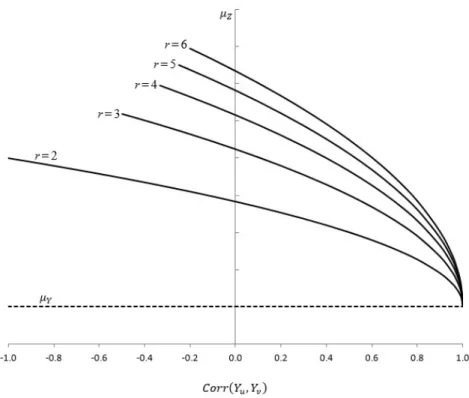
To illustrate the effect of arc travel-time correlation on route travel-time correlation, suppose we have two routes with the same number of arcs in each (i.e.,n = m) and that the variances of the travel times for all arcs are equal (σ_i =σ_j ∀i, j). Further assume that the magnitude – but not necessarily the sign – of the correlation coefficients are the same. Equation (5) then reduces to:

Corr(Y1, Y2) = _{1 + (n}nρ₋ij_1)ρ

ik. (6)

Figure 1 illustrates the correlation of route times when the correlations of arc times are positive within a route (ρ_ij) and either positive (ρ_ik = ρ_ij) or negative (ρ_ik = −ρ_ij) between routes. Ifn = 1, the route correlation is the arc correlation. However, the corre-lation of route times approaches one as the number of arcs in the routes increases. And the effect is substantial even for the size of problems typically encountered in routing prob-lems; for a arc correlation ofρ_ij = 0.20, the route correlation equals0.60forn = 6arcs. So even weakly correlated arc travel times can result in strongly correlated route times that we must deal with in designing routes. And when the variances and correlations are not the same for all arcs, we can take advantage of these relationships in designing routes by appropriately assigning arcs to routes to influence the route correlations to our advantage.

3.2

Effect of Route Correlation on the Makespan

Once the arcs have been assigned to routes, the mean and variance of each route as well as their correlation can be calculated as discussed in the previous section. So we now turn our attention to determining the effect of correlated route times on the makespan. The exact distribution of the maximum of two correlated, non-IID, Gaussian random variables, Z =max{Y1 ∼ N(μY1, σY21), Y2 ∼ N(μY2, σY22)}is known (Nadarajah and Kotz, 2008).

The meanμ_Z and the varianceσ_Z2 are:

μZ = μY1Φ[α] +μY2Φ[−α] +σΔYφ[α] (7)

σ2

Figure 1: Correlation of Route Times for Identically-distributed Arc Travel Times where: σΔY = σ2 Y1 +σY22 −2σY1σY2Corr(Y1, Y2) (9) α = (μY1 −μY2) σΔY , (10)

and whereφandΦare the density and cumulative distribution functions for the standard normal distribution, respectively, and the correlation between the two routes,Corr(Y1, Y2), is obtained from (5).

To isolate the effect of correlated route times on the makespan, suppose the two routes have equal means and variances, μ_Y1 = μ_Y2 = μ_Y and σ2_Y1 = σ2_Y2 = σ2_Y. Then, from Equation 9:

σΔY =

2σ2

Y[1−Corr(Y1, Y2)]. (11) For equal means,α= 0, and for a normal distribution,Φ[0] = 0.5andφ[0] = √1

2π, so the expected value of the maximum of the two routes will be:

μZ =μY +σΔY

1−Corr(Y1, Y2)

π . (12)

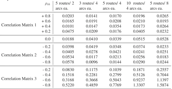
If the routes are perfectly positively correlated (i.e. Corr(Y1, Y2) = 1), the expected value of the maximum will simply be the mean of each route, since the two routes will always have the same time. However, as the correlation decreases, μ_Z increases rapidly as shown in Figure 2 (r = 2). In designing routes, we will likely not have route times with equal means and covariances, but we should take advantage of this effect of route correlation by assigning arcs to routes in such a manner as to maintain positive correlations among routes as much as possible.

Figure 2: Effect of Route Correlation on the Expected Value of the Makespan Figure 2 also provides the expected value of the makespan for three through six routes (based on tabulated values provided in Arnold et al. (2008)). However, for more than two routes, all of the routes cannot have a strong negative correlation. For example, if A is negatively correlated with B, and B is negatively correlated with C, we would ex-pect A to be positively correlated with C. More formally, a correlation matrix must be

positive semidefinite due to the fact that the variance must be positive (Rapisarda et al. (2007)). As indicated by David and Nagaraja (2003), for identically-distributed equicorre-lated multinormal variables, the common correlation coefficient must satisfy the following relationship:

−1

(r−1) ≤Corr(Yu, Yv)≤1, (13)

whereris the number of routes. Thus, the curves do not extend beyond this range. As illustrated in Figure 2, the effect of route correlation is even more pronounced as the number of routes increases. The judicious assignment of arcs to routes is critical when the arcs, and therefore the routes, are correlated. Of course, a routing application will not have equal means and covariances, but the assignment of arcs to routes must take into consideration not only the expected times of each route, but the variances and correlations as well. So we now turn our attention to the development of a general heuristic that incorporates the effects of arc correlation on route correlation and of route correlation on the makespan. In the next section, we describe a means of estimating the expected makespan for a given assignment. Then, we describe a heuristic for the min-mean-max vehicle routing problem.

4

Calculating the Expected Makespan and Standard

De-viation

Our intent is to develop a general heuristic to determine the expected value, or the ex-pected value plus one standard deviation, of the maximum travel time of several routes with correlated arc travel times. It should be able to be used in a variety of arc- and node-routing algorithms by simply replacing the objective-function computation with the proposed heuristic, and it should easily be incorporated as part of general-purpose software if so desired.

In reviewing the literature on the distributional properties of trips, Noland and Po-lak (2002) found evidence of normally and lognormally distributed travel times. Taylor (1999) notes that the normal distribution is appropriate for heavily-congested arcs, but the lognormal distribution better describes less congested arcs. Chiang and Roberts (1980) found that a shifted gamma distribution provides reasonable estimates of the travel time for regular-route, less-than-truckload trucking. For normally-distributed arc travel times, the route times will also be normally distributed; for non-normal arc travel times, the route time may tend toward a normal distribution, but the number of arcs in a route may not be sufficient for the Central Limit Theorem to assure convergence to the normal.

However, even if all of the route times are approximately normal, the distribution of the maximum time will not be normal; in fact, it will be skewed. The asymptotic limit distribution of the maximum of IID normal variables is the Gumbel distribution. However, a typical routing problem will not likely have enough routes to converge to the Gumbel distribution, and the route times will neither be identical nor, due to the correlated arc times as illustrated in the previous section, independent.

For two routes with normally-distributed route times, the expected value of the maxi-mum route time can be taken directly from equation (7) above. For more than two routes and/or for non-normal route times, some authors (beginning with Clark (1961)) have sug-gested a recursive algorithm using extreme-value theory to estimate the expected maxi-mum value. For the routing problem under consideration, this process is incorporated into our proposed approximation algorithm as follows.

4.1

An Approximation Algorithm

LetΠ_p be a set of arcs in routep(a given assignment of arcs to routes). Suppose the travel time on each arc follows an arbitrary distribution with a mean ofμ_i and a variance ofσ2_i as well as a correlation of the time to travel arci and arck ofρ_ik (i, k ∈ Π_p); hence the covariance isσ_ik =ρ_ikσ_iσ_k, whereσ_ii =σ_i2 andρ_ii= 1.

Step 1: Initial mean and variance of routes. Calculate the mean and variance of the time to complete each route (whereR_p is the time to complete routep, and using indices iandkfor routepwithn_parcs assigned to it). Then, for each routep:

E(Rp) = np i=1 μi (14) V ar(Rp) = np i=1 np k=1 σik = np i=1 np k=1 ρikσiσk (15) Step 2: Initial correlation between the routes. Calculate the correlation coefficient of the time to complete each pair of routes (using indices i and k for route p with np arcs assigned to it, and using indicesj andl for routeqwithnqarcs). Then, for each pair of routespandq:

Corr(Rp, Rq) = _np i=1 _np+nq j=np+1ρijσiσj _np i=1 _np k=1ρikσiσkjn=p+npn+1q _np+nq l=np+1ρjlσjσl (16)

At this point, we have the distribution of the time to complete each route. To simplify subsequent expressions, letμ_Rp =E(R_p)be the expected (mean) time to complete routep, andσ_R2_p =V ar(R_p)be the variance of the time to complete routep.

Step 3: Mean and variance for a first combination of routes. Calculate the mean and variance of the maximum time to complete the first two routes. LetA=max{R1, R2}, andν_A1 andν_A2 be the first and the second moment ofA, respectively:

νA1 = μR1Φ[α] +μR2Φ[−α] +σΔRφ[α] (17) νA2 = (μ2R1 +σR21)Φ[α] + (μ2R2 +σR22)Φ[−α] + (μR1 +μR2)σΔRφ[α] (18) where σΔR = σ2 R1 +σ2R2 −2σR1σR2Corr(R1, R2) (19) α = (μR1 −μR1) σΔR (20)

andφ andΦare the density and cumulative distribution functions for the standard normal distribution, respectively.

Then, the mean and variance of the maximum of the two route times will beμ_A = νA1 andσ2A=νA2 −νA21.

Step 4: Recompute correlation coefficients. Calculate the correlation coefficient of A and each of the remaining routes (forp= 3,4, ...):

Corr(A, Rp) = σR1Corr(R1, Rp)Φ[α] +σR2Corr(R2, Rp)Φ[−α] νA2 −νA21

(21)

Step 5: Further recombination of routes. TreatAas a normally-distributed route (even though it is not) and calculate the mean and variance of the maximum ofA and a third route; that is,B =max{R1, R2, R3}=max{A, R3}:

νB1 andνB2 can be calculated as in Step 3, replacingμR1 andσR21 withμAandσ2A,

respectively, and replacingμ_R2 andσ_R2₂ withμ_R3 andσ_R2₃, respectively.

Step 6: Further recalculation of correlation coefficients. Calculate the correlation co-efficient ofB and each of remaining routes (forp= 4,5, ...):

Corr(B, Rp) = σACorr(RA, Rp)Φ[α] +σR3Corr(R3, Rp)Φ[−α] νB2 −νB21

(22)

Note that this will require the use of the correlations in Step 4.

Step 7: Recursion. Repeat Steps 5 and 6 until all routes have been included (C = max{B, R4}, D = max{C, R5}, etc.). The final values of the mean and variance of the makespan can then be determined from equations (17) and (18).

4.2

Evaluating the Accuracy of the Approximation

For two routes with normally-distributed arc travel times, equations (17) and (18) will provide an exact solution. To evaluate the accuracy of the approximating algorithm for more than two routes and/or for non-normal route times, we compare the results of the algorithm with simulated results. We consider various numbers of routes, routes with varying numbers of arcs as well as various travel-time distributions.

The distributions, including the mean and coefficient of variation, of the arc travel times are randomly generated in the manner of Ehmke et al. (2015). The distance between each pair of customers is the Euclidean distance between randomly-generated coordinates in two-dimensional space with a uniform distribution between0and40. The mean travel time is set equal to this distance, while the coefficient of variation is randomly gener-ated with a uniform distribution between0.1and0.3. Three travel-time distributions are evaluated – a normal distribution, a shifted gamma distribution, and a shifted exponential distribution – with parameters set such that the appropriate mean and coefficient of vari-ation are obtained with a skewness equal to 0(normal), 1(shifted gamma), or 2(shifted exponential). Five instances for each test scenario are generated.

In addition to the situation with uncorrelated travel times (an identity correlation ma-trix), three types of correlation matrices were constructed for evaluation. For the first scenario, the travel times for all arcs are assumed to be positively equicorrelated; four val-ues representing increasing interrelationships are used (ρ_ik = +0.2,+0.4,+0.6,and+0.8, fori =k). The other two scenarios incorporate negative correlations; however, due to the need for a positive semidefinite correlation matrix, some of the correlation coefficients are necessarily positive. The second scenario is such that the travel times are positively and negatively correlated within a route and with arcs in all other routes. The third scenario is such that the travel times are positively correlated within a route and positively correlated with all arcs in half of the other routes, negatively correlated with arcs in the other half of

the routes. Tables 1–3 of the electronic appendix illustrate the three types of matrices for a3route/4arcs per route instance with a correlation coefficient of0.2.

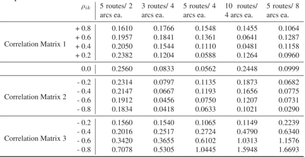
To measure its accuracy, the expected makespan of the approximation algorithm is compared to the results of a simulation using @Risk with 10,000 simulation runs. Ta-bles 1–3 provide the mean absolute percent error (MAPE) of the five instances for each test scenario. Results are provided for 3, 5, and 10 routes; for 2, 4, and 8 arcs per route; as well as for normal, shifted gamma, and shifted exponential travel-time distributions. Table 1: Mean Absolute Percent Deviation of the Algorithm vs. Simulated Expected Makespan – Normal Distribution

ρik 5 routes/ 2 arcs ea. 3 routes/ 4 arcs ea. 5 routes/ 4 arcs ea. 10 routes/ 4 arcs ea. 5 routes/ 8 arcs ea. Correlation Matrix 1 + 0.8 0.0203 0.0141 0.0170 0.0196 0.0265 + 0.6 0.0165 0.0191 0.0208 0.0210 0.0193 + 0.4 0.0101 0.0147 0.0354 0.0173 0.0264 + 0.2 0.0475 0.0209 0.0176 0.0405 0.0232 0.0 0.0188 0.0410 0.0339 0.0515 0.0528 Correlation Matrix 2 - 0.2 0.0398 0.0419 0.0348 0.0374 0.0233 - 0.4 0.0405 0.0278 0.0421 0.0241 0.0251 - 0.6 0.0534 0.0117 0.0213 0.0256 0.0183 - 0.8 0.0578 0.0096 0.0144 0.0290 0.0244 Correlation Matrix 3 - 0.2 0.0830 0.1175 0.1039 0.1871 0.2557 - 0.4 0.1518 0.2281 0.2799 0.5126 0.7044 - 0.6 0.3168 0.3668 0.5043 0.9237 1.1397 - 0.8 0.5220 0.4859 0.7769 1.3307 1.5874 As illustrated in Tables 1–3, the algorithm is remarkably accurate in estimating the expected makespan. For normally-distributed travel times (Table 1), all of the MAPEs for Correlation Matrices 1 and 2 are less than one-tenth of one percent, with no apparent effect of the number of routes or the number of arcs per route. Not surprisingly, the accuracy is slightly less for the gamma and exponential distributions (Tables 2 and 3), although there is still less than one-half of one percent error for Correlation Matrices 1 and 2. For these distributions, increasing the number of arcs per route (e.g., going from 2 to 4 to 8 arcs per route with 5 routes) improves the accuracy of the algorithm, likely due to the fact that the route times approach normality as the number of arcs grows larger.

The results from Correlation Matrix 3 are somewhat different. Although the algo-rithm is still reasonably accurate – MAPEs within 1.6, 1.7, and 2.6 percent for the normal, shifted gamma, and shifted exponential travel-time distributions, respectively – the errors are consistently higher. While it is not apparent as to why the algorithm is relatively less

Table 2: Mean Absolute Percent Deviation of the Algorithm vs. Simulated Expected Makespan – Shifted Gamma Distribution

ρik 5 routes/ 2 arcs ea. 3 routes/ 4 arcs ea. 5 routes/ 4 arcs ea. 10 routes/ 4 arcs ea. 5 routes/ 8 arcs ea. Correlation Matrix 1 + 0.8 0.1610 0.1766 0.1548 0.1455 0.1064 + 0.6 0.1957 0.1841 0.1361 0.0641 0.1287 + 0.4 0.2050 0.1544 0.1110 0.0481 0.1158 + 0.2 0.2382 0.1204 0.0588 0.1264 0.0960 0.0 0.2560 0.0833 0.0562 0.2448 0.0999 Correlation Matrix 2 - 0.2 0.2314 0.0797 0.1135 0.1873 0.0682 - 0.4 0.2147 0.0667 0.1193 0.1656 0.0775 - 0.6 0.1912 0.0456 0.0750 0.1207 0.0731 - 0.8 0.1834 0.0418 0.0633 0.1021 0.0290 Correlation Matrix 3 - 0.2 0.1560 0.1540 0.1065 0.1149 0.2239 - 0.4 0.2016 0.2517 0.2724 0.4790 0.6340 - 0.6 0.3420 0.3655 0.6102 1.0313 1.1576 - 0.8 0.7078 0.5305 1.0445 1.5948 1.6693

Table 3: Mean Absolute Percent Deviation of the Algorithm vs. Simulated Expected Makespan – Shifted Exponential Distribution

ρik 5 routes/ 2 arcs ea. 3 routes/ 4 arcs ea. 5 routes/ 4 arcs ea. 10 routes/ 4 arcs ea. 5 routes/ 8 arcs ea. Correlation Matrix 1 + 0.8 0.3335 0.3009 0.1845 0.2567 0.1444 + 0.6 0.3524 0.3007 0.1988 0.1753 0.1553 + 0.4 0.3612 0.2722 0.1856 0.1431 0.1396 + 0.2 0.3494 0.2231 0.1677 0.1963 0.1384 0.0 0.4004 0.1713 0.1994 0.3968 0.1310 Correlation Matrix 2 - 0.2 0.4331 0.1573 0.2478 0.3627 0.1604 - 0.4 0.4402 0.1278 0.2849 0.3035 0.1407 - 0.6 0.3925 0.1079 0.2587 0.2485 0.0918 - 0.8 0.3274 0.0913 0.2081 0.2612 0.0699 Correlation Matrix 3 - 0.2 0.6288 0.6507 0.6340 0.9166 0.8230 - 0.4 0.4578 0.5062 0.7393 0.7834 0.9837 - 0.6 0.9347 0.8008 1.3129 1.5489 1.7297 - 0.8 1.5093 1.1784 1.9794 2.4415 2.5177

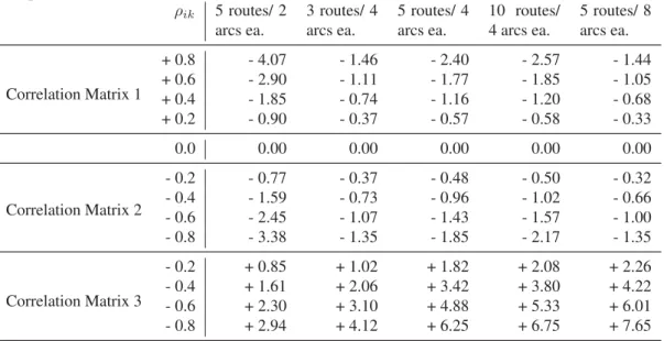
effective in this situation, it is interesting to note that Correlation Matrices 1 and 2 provide expected makespans that are smaller than the uncorrelated case (ρ_ik = 0), while Corre-lation Matrix 3 results in larger makespans (as shown in Table 4). CorreCorre-lation Matrix 1 has fairly high, positively-correlated route times, which decreases the expected makespan (see Figure 2). Correlation Matrix 2 has positively- and negatively-correlated arcs within a route, resulting in a lower variance, and also results in route times that have low correla-tions. Correlation Matrix 3, on the other hand, results in relatively highly-correlated route times, some of which are negative; therefore, increasing the expected makespan. Again, this highlights the need for an appropriate routing algorithm that can take advantage of correlated travel times.

Table 4: Mean Percent Deviation of the Expected Makespan from the Uncorrelated Makespan ρik 5 routes/ 2 arcs ea. 3 routes/ 4 arcs ea. 5 routes/ 4 arcs ea. 10 routes/ 4 arcs ea. 5 routes/ 8 arcs ea. Correlation Matrix 1 + 0.8 - 4.07 - 1.46 - 2.40 - 2.57 - 1.44 + 0.6 - 2.90 - 1.11 - 1.77 - 1.85 - 1.05 + 0.4 - 1.85 - 0.74 - 1.16 - 1.20 - 0.68 + 0.2 - 0.90 - 0.37 - 0.57 - 0.58 - 0.33 0.0 0.00 0.00 0.00 0.00 0.00 Correlation Matrix 2 - 0.2 - 0.77 - 0.37 - 0.48 - 0.50 - 0.32 - 0.4 - 1.59 - 0.73 - 0.96 - 1.02 - 0.66 - 0.6 - 2.45 - 1.07 - 1.43 - 1.57 - 1.00 - 0.8 - 3.38 - 1.35 - 1.85 - 2.17 - 1.35 Correlation Matrix 3 - 0.2 + 0.85 + 1.02 + 1.82 + 2.08 + 2.26 - 0.4 + 1.61 + 2.06 + 3.42 + 3.80 + 4.22 - 0.6 + 2.30 + 3.10 + 4.88 + 5.33 + 6.01 - 0.8 + 2.94 + 4.12 + 6.25 + 6.75 + 7.65

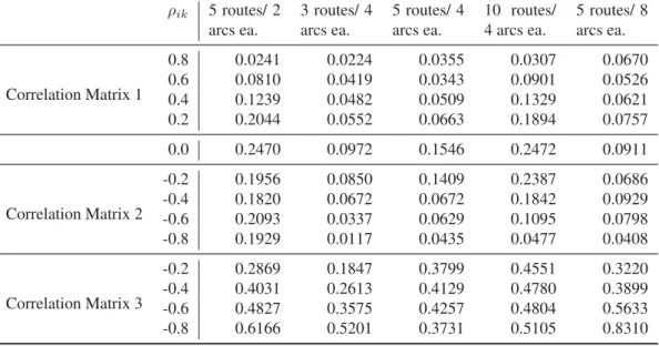
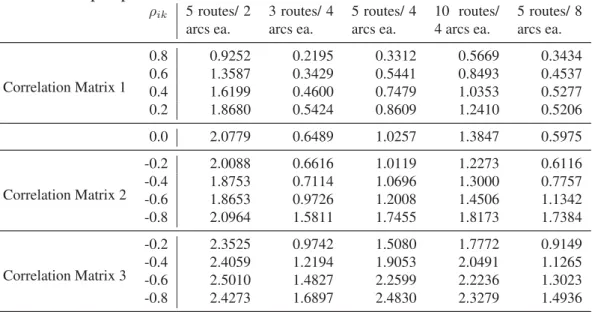
While the expected makespan determined from the approximation algorithm is quite accurate, the same cannot be said of the makespan variance. Thus, to consider an objective that combines the mean as well as the variability, we evaluate the accuracy of the expected value plus one standard deviation of the makespan. As seen in Table 5, the approximation algorithm provides solutions for normally-distributed travel times that are within one per-cent of the simulated values for all instances. In fact, some instances are better than the deviation of the expected value alone, as an underestimated standard deviation somewhat offsets an overestimated mean. Tables 6 and 7 provide the results for the shifted gamma and shifted exponential distributions. In these situations, the estimate of the makespan variance is considerably worse than that realized with the normal distribution. Thus, the

mean absolute percent deviation of the expected value plus one standard deviation of the makespan is as high as 2.5% for the shifted gamma and as high as 4.5% for the shifted exponential.

Table 5: Mean Absolute Percent Deviation of the Approximation Algorithm vs. Simulated Expected Makespan plus Standard Deviation – Normal Distribution

ρik 5 routes/ 2 arcs ea. 3 routes/ 4 arcs ea. 5 routes/ 4 arcs ea. 10 routes/ 4 arcs ea. 5 routes/ 8 arcs ea. Correlation Matrix 1 0.8 0.0241 0.0224 0.0355 0.0307 0.0670 0.6 0.0810 0.0419 0.0343 0.0901 0.0526 0.4 0.1239 0.0482 0.0509 0.1329 0.0621 0.2 0.2044 0.0552 0.0663 0.1894 0.0757 0.0 0.2470 0.0972 0.1546 0.2472 0.0911 Correlation Matrix 2 -0.2 0.1956 0.0850 0.1409 0.2387 0.0686 -0.4 0.1820 0.0672 0.0672 0.1842 0.0929 -0.6 0.2093 0.0337 0.0629 0.1095 0.0798 -0.8 0.1929 0.0117 0.0435 0.0477 0.0408 Correlation Matrix 3 -0.2 0.2869 0.1847 0.3799 0.4551 0.3220 -0.4 0.4031 0.2613 0.4129 0.4780 0.3899 -0.6 0.4827 0.3575 0.4257 0.4804 0.5633 -0.8 0.6166 0.5201 0.3731 0.5105 0.8310

5

A Vehicle Routing Heuristic

In Section 4, we presented an approach that approximates the expected makespan and the standard deviation based on extreme-value theory. Next, we want to embed this approx-imation within a vehicle routing algorithm to find the assignment of customers to routes that optimize the makespan (with and without standard deviation). In this section, we demonstrate how to integrate this approximation in the creation of routes for a fleet of ve-hicles. To this end, we use a well-known construction heuristic and improve the resulting set of routes by applying two adapted variants of standard local search neighborhoods. Step 1: Create Input Data. We create the the correlation matrix and the covariance

ma-trix for a given set of depot, customers and their locations to prepare the data input required for the approximation approach presented in Section 4.

Step 2: Initialize Routes. For the creation of routes, we assume that the number of routes is given, and we aim at creating routes for our makespan objective (with or without

Table 6: Mean Absolute Percent Deviation of the Approximation Algorithm vs. Simulated Expected Makespan plus Standard Deviation – Gamma Distribution

ρik 5 routes/ 2 arcs ea. 3 routes/ 4 arcs ea. 5 routes/ 4 arcs ea. 10 routes/ 4 arcs ea. 5 routes/ 8 arcs ea. Correlation Matrix 1 0.8 0.9252 0.2195 0.3312 0.5669 0.3434 0.6 1.3587 0.3429 0.5441 0.8493 0.4537 0.4 1.6199 0.4600 0.7479 1.0353 0.5277 0.2 1.8680 0.5424 0.8609 1.2410 0.5206 0.0 2.0779 0.6489 1.0257 1.3847 0.5975 Correlation Matrix 2 -0.2 2.0088 0.6616 1.0119 1.2273 0.6116 -0.4 1.8753 0.7114 1.0696 1.3000 0.7757 -0.6 1.8653 0.9726 1.2008 1.4506 1.1342 -0.8 2.0964 1.5811 1.7455 1.8173 1.7384 Correlation Matrix 3 -0.2 2.3525 0.9742 1.5080 1.7772 0.9149 -0.4 2.4059 1.2194 1.9053 2.0491 1.1265 -0.6 2.5010 1.4827 2.2599 2.2236 1.3023 -0.8 2.4273 1.6897 2.4830 2.3279 1.4936

Table 7: Mean Absolute Percent Deviation of the Approximation Algorithm vs. Simulated Expected Makespan plus Standard Deviation – Exponential Distribution

ρik 5 routes/ 2 arcs ea. 3 routes/ 4 arcs ea. 5 routes/ 4 arcs ea. 10 routes/ 4 arcs ea. 5 routes/ 8 arcs ea. Correlation Matrix 1 0.8 1.5588 0.3085 0.5311 0.9059 0.5998 0.6 2.2931 0.4176 0.8448 1.3469 0.7432 0.4 2.7512 0.5392 1.1494 1.7126 0.8267 0.2 3.1825 0.8281 1.4687 1.9562 0.8605 0.0 3.6130 1.1555 1.8766 2.3290 1.0586 Correlation Matrix 2 -0.2 3.5489 1.2247 1.9359 2.3337 1.2421 -0.4 3.6662 1.6979 2.2456 2.6489 1.8506 -0.6 3.8829 2.5114 2.9628 3.2389 2.7830 -0.8 4.4062 3.8882 4.0853 4.0865 4.0980 Correlation Matrix 3 -0.2 3.9053 1.4024 2.6043 2.6593 1.5607 -0.4 3.8939 1.7617 2.8401 3.0395 1.7323 -0.6 3.9030 2.1995 3.2908 3.2957 2.1317 -0.8 3.8615 2.6201 3.6430 3.5390 2.5300

standard deviation) for the given number of routes. We initialize the routes by as-signing the farthest, second-farthest, etc. customers to the routes until every route has one initial customer.

Step 3: Insert Customers. We insert the remaining customers following the idea of a greedy randomized adaptive search (GRASP). In each insertion step, we evaluate the consequences of insertion for our complex makespan objective for all remaining customers, routes and insertion positions in these routes. Out of the three “best” customers and insertion points, we randomly choose one for insertion. We continue until all customers have been assigned. We evaluate the current solution with the approximation approach of Section 4 whenever we check if an insertion to a partic-ular insertion point would be beneficial or not. In the end, all customers have been inserted, and a first feasible solution has been created. Due to the random nature of our GRASP approach, we repeat the construction of the initial route plan five times and improve the best of the five created route plans as follows.

Step 4: Improve Routes (1-shift). The created initial solution is subject to improvement with standard local search neighborhood operators. First, we apply the idea of 1-shift, which investigates whether it is beneficial to shift a customer from its current position to all other possible insertion points within the same or the other routes. We identify the most beneficial shift with regard to our objective, keep the improved solution, and continue with 1-shift operations as long as we can find improvements. Step 5: Improve Routes (Exchange). We use the well-known exchange operator to sys-tematically switch two customers between different routes. We compute the conse-quences that each switch would have on our makespan objective (with or without standard deviation) and perform the first exchange that leads to an improvement. If we found an improvement, we start the exchange operator again. We continue the exchange operator until no improvement of the objective function is possible any more. Then, we activate 1-shift again, and both operators run alternately until we cannot find improved solutions any more.

Complete evaluation of the current solution is necessary whenever we analyze the conse-quences of an insertion or a local search move. This leads to a significant increase in run times compared to deterministic routing objectives, where it is often sufficient to perform a delta comparison to evaluate the suitability of a local search move.

6

Experimental Design and Results

In this section, we introduce the instances and present the computational results of our stochastic vehicle routing algorithm.

6.1

Instances

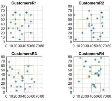
We analyze the impact of correlation in optimizing routes based on well-known benchmark instances with correlation patterns motivated by literature on correlation. In particular, we use the dataset R101 of the Solomon datasets. We use the first customer as depot location. We form four sets of instances based on the next 20 customers, i.e., depot location and customers 2, 3, ..., 21 form the instance R101-1 (short: R1), 22, 23, ..., 41 form R101-2 (short: R2), etc. We focused on fairly small instances so that we could understand and visualize the impact of the correlation on vehicle routing. Solutions for every instance are generated according to the following correlation scenarios:

• Scenario typeincidents (INC): Guo (2006) suggests arc travel times may be corre-lated due to weather effects and secondary incidents. Zockaie et al. (2016) consider different incidents to produce travel time variations in each scenario. In addition, our motivation comes from the real life observation that traffic incidents may often create local traffic jams that are not observed on a regular day-to-day basis. Hence, for the incident scenario, we define three locations of “incidents” randomly in the Euclidean plane. We assume that there is positive correlation between all arcs within 5 unit blocks of the incident locations. If arcs start or finish in the same block, they are positively correlated. This is illustrated in Figure 3.

• Scenario type inner/outer (I/O): Nicholson (2015) suggests that negative correla-tion can occur when a bottleneck in one locacorrela-tion results in increased speeds on the downstream locations. This motivates us to consider an inner/outer scenario: if dur-ing a given time period a large amount of traffic is godur-ing into the same direction, the reverse direction is more likely to be less loaded. Hence, for our scenario, we designate a block in the middle of the investigated area (coordinates 20-50, 20-50) to be the “downtown”. All arcs into the downtown block are positively correlated and all arcs out of the downtown block are positively correlated. The two groups are negatively correlated (i.e. if they are going into different directions). This is illustrated in Figure 4.

We conduct experiments for the above instances and scenarios for four different cor-relation coefficients, namely zero corcor-relation, 0.5, 0.75 and 0.9 (for negative corcor-relation

Figure 3: Setup for INC Scenario

the negative of this). We also consider different coefficient of variation levels of travel times: 25% of mean, 50% of mean, 75% of mean. We assume a normal distribution on travel times. The number of vehicles is fixed and is either 3 or 5. Finally, we investigate two different parameterizations of our objective function (makespan with/without standard deviation). For each result, we report the objective function value and the individual com-ponents, i.e. the makespan and standard deviation, and compare it to the zero-correlation solutions.

We implemented our algorithms in Java 8 on a laptop with Win10 OS, Intel i7-7700HQ processor and 16 GB of RAM. We observed that the runtime heavily depends on the num-ber of vehicles. The computation of one solution for a three-vehicle instance takes roughly 30 minutes and is about one hour for a five-vehicle instance.

6.2

Results

We first present summary tables and then discuss illustrative examples of routes created with our stochastic routing algorithm.

6.2.1 Summary Tables

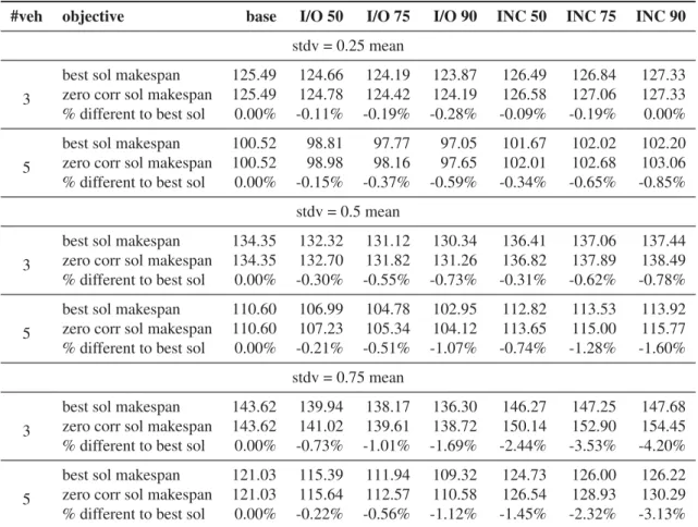
Summary results are given in Tables 8–9. Detailed results are in the electronic appendix in Tables 4–9. For Table 8, we will first define the columns: #veh refers to the number of vehicles used, objective refers to the objective of the routing problem solved, base refers to the no correlation case,I/O 50, I/O 75, I/O 90refer to the corresponding inner-outer correlation matrix with 0.5/-0.5, 0.75/-0.75, 0.9/-0.9 correlation values, respectively, and INC 50, INC 75, INC 90 refer to the corresponding incidence correlation matrix with 0.5/-0.5, 0.75/-0.75, 0.9/-0.9 correlation values, respectively. In terms of the rows, stdv=0.* meanis where∗is the ratio of the standard deviation of travel time to the mean for each arc (i.e. coefficient of variation),best sol makespanis the expected makespan of the best solution obtained for the given correlation matrix,zero corr sol makespanis the expected makespan of the zero correlation solution evaluated using the given correlation matrix, and % different to best solution is the percentage difference between the best solution for expected makespan and the zero correlation solution evaluated with the given correlation matrix (i.e. the savings in expected makespan from including correlation in our routing algorithm).

From Table 8 that only considers expected makespan, a few patterns are apparent. Increasing the correlation across each correlation scenario leads to increased importance in modeling the correlation in the routing. For example, for 5 vehicles and stdv=0.25 mean, we see savings of 0.34%, 0.65%, and 0.85% for INC 50, INC 75, and INC 90. This is

not surprising since more correlation should yield larger impact on solutions. We also see that a larger coefficient of variation yields larger impacts from modeling correlation. For example, for I/O 50 and 3 vehicles, we see the savings go from 0.11% to 0.30% to 0.73% as the standard deviation increases. We will look at an example with a coefficient of variation of 0.75 in the next section to understand the changes in the routes creating the savings. In general, there is no strong relationship between the number of vehicles and the savings from modeling correlation. We see that with 20 customers most experiments yield an average savings of around 1% or less except with the highest coefficient of variation and the INC correlation scenarios. Here we see values ranging as high as 4.20% average improvement from modeling correlation.

Next, we will consider Table 9 that optimizes for expected makespan plus standard deviation. The columns are the same as for Table 8, but there are additional rows. These include best sol stdv which is the standard deviation of the best solution obtained the given correlation matrix, best sol ms+stdvthe sum of the makespan and standard devia-tion of the best soludevia-tion obtained for the given correladevia-tion matrix, zero corr sol stdvthe standard deviation of the zero correlation solution evaluated using the given correlation matrix, zero corr sol ms+stdv makespan plus standard deviation of the zero correlation solution evaluated using the given correlation matrix, and% difference to best solution now represents percentage difference between the zero correlation solution evaluated with the given correlation matrix and the best solution for expected makespan and standard deviation.

Here, we observe generally larger average savings from considering correlation. This is particularly apparent for the INC scenario as we create average savings as high as 2.54% even with a coefficient of variation of only 0.25. We note that the highest average savings across the table is 4.38%, though, which is only slightly higher than 4.20% in Table 8, but many more values in the tables have savings more than 1%. We again see savings increase when considering correlation, but not so clearly with increasing coefficient of variation. This seems to be a change created by the new objective. The dramatic increase in magnitude of savings when incorporating correlation with the INC scenarios is quite interesting and is one of the patterns we try to understand better in the next section.

We can also observe differences in the components of the combined objective. In Table 9, we see that the solutions found with the combined objective sometimes have larger expected makespans than the zero correlation solutions (when evaluated with the same correlation matrix), but almost always have an equal or smaller standard deviation (only exceptions are 3 and 5 vehicles, coefficient of variation of 0.25, I/O 50).

Table 8: Summary Results for Minimizing Makespan

#veh objective base I/O 50 I/O 75 I/O 90 INC 50 INC 75 INC 90

stdv = 0.25 mean

3

best sol makespan 125.49 124.66 124.19 123.87 126.49 126.84 127.33 zero corr sol makespan 125.49 124.78 124.42 124.19 126.58 127.06 127.33 % different to best sol 0.00% -0.11% -0.19% -0.28% -0.09% -0.19% 0.00%

5

best sol makespan 100.52 98.81 97.77 97.05 101.67 102.02 102.20 zero corr sol makespan 100.52 98.98 98.16 97.65 102.01 102.68 103.06 % different to best sol 0.00% -0.15% -0.37% -0.59% -0.34% -0.65% -0.85%

stdv = 0.5 mean

3

best sol makespan 134.35 132.32 131.12 130.34 136.41 137.06 137.44 zero corr sol makespan 134.35 132.70 131.82 131.26 136.82 137.89 138.49 % different to best sol 0.00% -0.30% -0.55% -0.73% -0.31% -0.62% -0.78%

5

best sol makespan 110.60 106.99 104.78 102.95 112.82 113.53 113.92 zero corr sol makespan 110.60 107.23 105.34 104.12 113.65 115.00 115.77 % different to best sol 0.00% -0.21% -0.51% -1.07% -0.74% -1.28% -1.60%

stdv = 0.75 mean

3

best sol makespan 143.62 139.94 138.17 136.30 146.27 147.25 147.68 zero corr sol makespan 143.62 141.02 139.61 138.72 150.14 152.90 154.45 % different to best sol 0.00% -0.73% -1.01% -1.69% -2.44% -3.53% -4.20%

5

best sol makespan 121.03 115.39 111.94 109.32 124.73 126.00 126.22 zero corr sol makespan 121.03 115.64 112.57 110.58 126.54 128.93 130.29 % different to best sol 0.00% -0.22% -0.56% -1.12% -1.45% -2.32% -3.13%

Table 9: Summary Results for Minimizing Makespan plus Standard Deviation #veh objective base I/O 50 I/O 75 I/O 90 INC 50 INC 75 INC 90

stdv = 0.25 mean

3

best sol makespan 127.67 126.44 125.89 125.49 126.49 126.84 127.04 best sol stdv 9.08 8.15 7.49 7.06 11.65 12.38 12.79 best sol ms+stdv 136.75 134.59 133.38 132.55 138.14 139.22 139.83 zero corr sol makespan 127.67 126.91 126.50 126.24 128.78 129.24 129.49 zero corr sol stdv 9.08 8.01 7.81 7.52 12.17 13.42 14.12 zero corr sol ms+stdv 136.75 134.93 134.32 133.77 140.95 142.66 143.60 % different to best sol 0.00% -0.24% -0.71% -0.94% -1.98% -2.35% -2.54%

5

best sol makespan 102.39 100.81 99.93 99.33 103.62 103.92 104.11 best sol stdv 8.06 6.88 6.15 5.37 8.91 9.31 9.53 best sol ms+stdv 110.45 107.68 106.08 104.70 112.53 113.23 113.63 zero corr sol makespan 102.39 100.87 100.12 99.68 103.93 104.62 105.02 zero corr sol stdv 8.06 6.87 6.19 5.72 9.32 9.93 10.29 zero corr sol ms+stdv 110.45 107.74 106.31 105.40 113.25 114.56 115.31 % different to best sol 0.00% -0.05% -0.20% -0.64% -0.65% -1.18% -1.47%

stdv = 0.5 mean

3

best sol makespan 134.55 132.66 131.28 131.63 136.57 137.23 137.62 best sol stdv 17.57 15.50 14.41 13.54 21.33 22.83 23.70 best sol ms+stdv 152.12 148.16 145.69 145.18 157.90 160.06 161.32 zero corr sol makespan 134.55 132.89 132.01 131.46 138.19 139.70 140.55 zero corr sol stdv 17.57 16.10 15.31 14.80 23.49 25.93 27.28 zero corr sol ms+stdv 152.12 149.00 147.32 146.27 161.67 165.63 167.83 % different to best sol 0.00% -0.58% -1.12% -0.68% -2.20% -3.17% -3.66%

5

best sol makespan 110.70 106.92 105.02 103.20 112.84 113.67 114.01 best sol stdv 14.62 12.17 10.57 9.28 16.54 17.22 17.76 best sol ms+stdv 125.32 119.10 115.59 112.48 129.38 130.89 131.77 zero corr sol makespan 110.70 107.29 105.38 104.15 113.97 115.44 116.28 zero corr sol stdv 14.62 12.42 11.20 10.44 17.45 18.88 19.72 zero corr sol ms+stdv 125.32 119.71 116.58 114.59 131.42 134.32 136.00 % different to best sol 0.00% -0.52% -0.81% -1.79% -1.54% -2.50% -3.03%

stdv = 0.75 mean

3

best sol makespan 143.29 140.26 138.31 137.51 146.28 147.54 149.02 best sol stdv 25.59 22.67 20.90 18.98 31.38 33.34 35.36 best sol ms+stdv 168.88 162.93 159.21 156.49 177.66 180.88 184.38 zero corr sol makespan 143.29 140.34 138.72 137.69 149.21 151.70 153.09 zero corr sol stdv 25.59 22.96 21.52 20.59 34.37 37.98 39.99 zero corr sol ms+stdv 168.88 163.29 160.24 158.29 183.58 189.68 193.08 % different to best sol 0.00% -0.20% -0.59% -1.03% -3.04% -4.38% -4.12%

5

best sol makespan 121.19 115.47 112.33 110.28 124.68 125.70 126.27 best sol stdv 21.43 18.07 15.36 12.55 24.44 25.53 26.18 best sol ms+stdv 142.61 133.54 127.69 122.83 149.11 151.23 152.45 zero corr sol makespan 121.19 116.03 113.11 111.20 126.31 128.61 129.92 zero corr sol stdv 21.43 18.12 16.26 15.09 25.92 28.13 29.41 zero corr sol ms+stdv 142.61 134.15 129.37 126.29 152.23 156.74 159.33 % different to best sol 0.00% -0.49% -1.32% -2.75% -2.01% -3.40% -4.15%

(a) No Correlation (b) INC Scenario Figure 5: Routes for R1, Makespan Objective 6.2.2 Illustrative Examples of Routes

To understand how correlation is causing these changes in solution values, we next ex-amine a series of illustrative examples. We will look at examples of how the different objectives and correlation patterns change the design of the routes. We will use instances with 3 vehicles and a coefficient of variation of 75%.

We start with the makespan objective and see how an incident correlation pattern changes the resulting routes. For R1 with a maximum positive correlation of 75%, the solution found for the incident correlation instance has a 2.65% improvement over using the routes from the no correlation version. A comparison of the routes found without cor-relation and with incident corcor-relation is in Figure 5. The two route plans are somewhat different: for instance, it can be observed that one of the customers at (42,48), who was assigned to route 1 with no correlation, has been reassigned to route 2 because of the fact that arcs coming to and leaving from that customer are positively correlated since they are starting and finishing in one of the incident locations.

For R2 with a maximum positive correlation of 90%, the solution found for the incident correlation instance has a 6.51% improvement over using the routes from the no correlation version. The routes found are in Figure 6. It is interesting to see that the solution with correlation here shows a crossing in the solution. The crossing is beneficial because the arcs are in the incident zone and become positively correlated as a result.

We can see the differences that inner/outer correlation can create for instance R3 (see Figure 7). For R3 with a maximum positive correlation of 90%, the solution found for the incident correlation instance has a 2.92% improvement over using the routes from the no

(a) No Correlation (b) INC Scenario Figure 6: Routes for R2, Makespan Objective

correlation version. For the inner/outer case, the customer that is the closest one to the depot gets reassigned to the different route due to its location inside of the downtown box. With standard deviation in the objective, we sometimes see similar changes as with only makespan, but at other times the routes change more. For R4, with a maximum positive correlation of 75%, the solution found for the incident correlation instance has a 5.73% improvement over using the routes from the no correlation version with just the makespan and 11.35% with makespan and standard deviation! The routes found with no correlation and the combined objective and the routes found with inner/outer correlation are in Figure 8. For this set of routes, the effect of the incident locations is the most visible. One can notice that all the routes look different in the base case and with the incident correlation. If we look at the top right incident location, we can see that route 1 changed such that the many customers present in route 1 in the base case are reassigned to a different route. We can also notice that those relocated customers were not in the incident location. This fact would suggest that correlation is important in this case and is the most influential. Here the moved customers are “close” to the customers in route 1 in the base case (which we typically want in a routing solution), but the impact of correlation is strong enough to put them on route 3 in the makespan plus standard deviation solution.

7

Summary and Future Work

Using ideas from extreme-value theory, we developed a method to incorporate arc travel time correlation in a vehicle routing problem with stochastic travel times. We integrated

(a) No Correlation (b) I/O Scenario Figure 7: Routes for R3, Makespan Objective

(a) No Correlation (b) INC Scenario

this approximation algorithm into a heuristic for the creation of routes for a fleet of ve-hicles. Using real world motivated scenarios, we explored the effect of the different cor-relation types/levels on the value of the objective function along with the set of resulting routes. We observed that correlation actually plays a significant role even for small in-stances with 20 customers and 3/5 vehicles. Taking correlation into account can result in an 11.35% decrease in the objective function value for these relatively small cases. These savings result from changes in the routes to take advantage of the impact of correlation that are counter-intuitive to typical route structures.

Future research directions include algorithmic and implementation improvements to decrease the computation time so that bigger datasets could be tested. Currently, we eval-uate the full objective for every change in the routes, but we will may be able to use clever storage techniques to make this faster. We also want to explore routing with different travel time distributions since our approximation algorithm showed the makespan to be accurate for distributions other than normal.

References

Adulyasak, Y. and P. Jaillet (2015). Models and algorithms for stochastic and robust vehicle routing with deadlines. Transportation Science 50(2), 608–626.

Ahr, D. and G. Reinelt (2006). A tabu search algorithm for the min–max k-chinese post-man problem. Computers & operations research 33(12), 3403–3422.

Akbari, V. and F. S. Salman (2017). Multi-vehicle synchronized arc routing problem to restore post-disaster network connectivity. European Journal of Operational Re-search 257(2), 625–640.

Ando, N. and E. Taniguchi (2006). Travel time reliability in vehicle routing and scheduling with time windows.Networks and spatial economics 6(3), 293–311.

Applegate, D., W. Cook, S. Dash, and A. Rohe (2002). Solution of a min-max vehicle routing problem. INFORMS Journal on Computing 14(2), 132–143.

Arkin, E. M., R. Hassin, and A. Levin (2006). Approximations for minimum and min-max vehicle routing problems.Journal of Algorithms 59(1), 1–18.

Arnold, B. C., N. Balakrishnan, and H. N. Nagaraja (2008). A first course in order statis-tics. SIAM.

Averbakh, I. and O. Berman (1997). (p- 1)(p+ 1)-approximate algorithms for p-traveling salesmen problems on a tree with minmax objective. Discrete Applied Mathemat-ics 75(3), 201–216.

Benavent, E., A. Corberan, I. Plana, and J. Sanchis (2014). Arc routing problems with min-max objectives. Arc Routing: Problems, Methods, and Applications; MOS-SIAM Series on Optimization, 255–280.

Benavent, E., A. Corber´an, I. Plana, and J. M. Sanchis (2009). Min-max k-vehicles windy rural postman problem. Networks 54(4), 216–226.

Benavent, E., ´A. Corber´an, and J. M. Sanchis (2010). A metaheuristic for the min– max windy rural postman problem with k vehicles. Computational Management Sci-ence 7(3), 269–287.

Bertazzi, L., B. Golden, and X. Wang (2015). Min–max vs. min–sum vehicle routing: A worst-case analysis. European Journal of Operational Research 240(2), 372–381.