DC Cable Short Circuit Fault Protection in VSC-MTDC

(1)

VSC-MTDC

Shining Lu

Wind Energy

Supervisor: Hans Kristian Høidalen, ELKRAFT Co-supervisor: Marjan Popov, TU Delft

Raymundo Torres, ELKRAFT

Department of Electric Power Engineering Submission date: June 2015

(2)

(3)

THESIS REPORT,

EUROPEAN WIND ENERGY MASTER PROGRAM, ELECTRIC POWER SYSTEM TRACK

DC Cable Short Circuit Fault

Protection in VSC-MTDC

By Shining Lu (4299841)

in partial fulfillment of the requirements for the degree of MSc Electrical Engineering at Delft University of Technology (TU Delft)

& MSc Technology – Wind Energy at Norwegian University of Science and Technology (NTNU) To be defended

on Monday, July 6th, 2015 at EWI/EEMCS faculty, TU Delft

Supervisors: Prof. Marjan Popov (TU Delft) Prof. Hans Kristian Høidalen (NTNU) Thesis Committee: Prof. Marjan Popov (TU Delft) Prof. Jose Rueda Torres (TU Delft) Prof. Armando Rodrigo Mor (TU Delft)

(4)

(5)

iii

Abstract

With the development of offshore wind farms, Voltage Source Converter based High Voltage Direct Current or Multi-terminal High Voltage Direct Current Technology (VSC-HVDC/MTDC) is becoming promising in the field of large-capacity and long-distance power transmission. However, its extreme vulnerability to DC contingencies remains a challenge in both research and practice. DC cable short circuit faults, or cable pole-to-pole faults, though less common than DC cable ground faults, can cause the most severe damage to the VSC as well as the whole system. In this thesis work, firstly a simple 3-terminal MTDC system is built and validated in PSCAD/EMTDC. Afterwards, based on the self-built MTDC system, DC cable short circuit faults with different locations are studied and analyzed in both theory and numerical simulation. Finally, a comprehensive protection scheme is proposed against such DC cable short circuit faults in the target MTDC system, combining the sub-schemes in fault detecting/locating principles, fault isolating tools and fault current limiting technologies. The coordination among the three parts is also taken into consideration. The scheme is later proven to be fast, selective, reliable, sensitive and robust in general. Moreover, the specific design procedure is further extended into a general design philosophy for DC cable short circuit fault protection in VSC-MTDC systems.

Keywords

(6)

(7)

v

Preface

This is the report for the master thesis ‘DC Cable Short Circuit Fault Protection in VSC-MTDC’ for European Wind Energy Master Program (EWEM), Electric Power System track. This project lasted from October 2014 to June 2015, with the work done partly in Norwegian University of Science and Technology (NTNU), Trondheim, Norway and partly in Delft University of Technology (TU Delft), Delft, the Netherlands.

Along with the emerging offshore wind farms, HVDC technology is becoming more and more attractive in high-capacity and long-distance transmission. On the other hand, the integration of wind farms is also widely acknowledged to be one of the most imminent applications in HVDC. Indeed, HVDC technology and wind energy interconnect and interact with each other. This is largely the reason why I chose this thesis topic to complete the two-year master study in EWEM. Although the report mainly falls into the electrical engineering field, the whole project roots in the context of a larger integration of wind energy and other sustainable resources in the future. The author also believes that the coming breakthroughs in HVDC as well as in other fields of electric power systems would contribute to further development in the wind energy industry.

Promising as the VSC-MTDC technology might be, it is also extremely vulnerable to DC contingencies, especially the pole-to-pole faults. During such faults, the diodes are usually considered to be the most critical component and that the fault current flowing through them cannot exceed 2 p.u.. In this thesis, a three-terminal VSC-MTDC system is built in PSCAD/EMTDC and a DC cable short circuit protection scheme is proposed for it. In the protection scheme, faults are detected by differential protection and/or wavelet-based fault detection, with overcurrent protection as the backup plan. Based on the data, the exact location of the fault can be further estimated by the travelling wave based fault locating principle. For fault isolation, three types of DC circuit breakers are introduced and the selection is made based on the coordination of the clearance time and the critical time limit with different diode sizing strategies. Above all, fault current limiters of both protective inductors on the DC side and the LCL circuit on the AC side are also implemented in the protection scheme to limit the overcurrent magnitude as well as to postpone the critical moment. Coordination among the three aspects of fault detecting/locating, fault isolating and fault current limiting are briefly discussed in the report as well, followed by a preliminary evaluation proving the proposed scheme to be fast, selective, reliable, sensitive and robust. Yet, the report also presents some suggestions in optimization and follow-up studies.

Throughout the thesis work, both model development, fault study and protection scheme design are illustrated with both theory and PSCAD simulation. Although the proposed scheme is based on a simple self-built three-terminal MTDC system, the general principle in protection system design should be similar for other grid topology. Nevertheless, particular issues might arise with the increase of terminal numbers and network complexity, or a change in VSC and cable configuration.

This work could not have been done without the help and support from many people, to whom I would like to extend my sincere gratitude here. Firstly, to my two supervisors, Professor Dr. Marjan Popov at TU Delft and Professor Dr. Hans Kristian Høidalen at NTNU, for providing the opportunity to study this interesting topic, as well as the valuable feedback throughout the work. The appreciation also goes to Lian Liu for his enthusiasm, patience and timely help in simulations; to Dr. Olimpo Anaya Lara and Dr. Raymundo Torres as well, for the guidance and assistance during my stay in NTNU. In addition, I also appreciate the valuable time and effort from the thesis committee, Dr. Marjan Popov (TU Delft supervisor), Dr. Jose Rueda Torres and Dr. Armando Rodrigo Mor. Last but not the least, thanks to the hugs and brownies; they will always be the warmest and sweetest memories of Europe.

Shining Lu 16/06/2015

(8)

vi

List of Figures

Figure 2.1 CIGRE B4 DC Grid Test System ... 4

Figure 2.2 Modified Three-terminal VSC-HVDC System Connected with DC Symmetrical Monopole Cable ... 5

Figure 2.3 System Layout in PSCAD/EMTDC Environment ... 5

Figure 2.4 Electrical Circuit Model Overview ... 6

Figure 2.5 AC Source Block Model ... 7

Figure 2.6 AC Filter Block Model ... 8

Figure 2.7 Phase Reactor Block Model ... 8

Figure 2.8 Two-level IGBT-VSC ... 9

Figure 2.9 PWM Modulation ... 9

Figure 2.10 VSC Station Electrical Subsystem ...10

Figure 2.11 VSC Controller Overview ...11

Figure 2.12 Inner Current Controller Models in PSCAD/EMTDC ...12

Figure 2.13 DC Voltage Controller (Outer Loop) ...13

Figure 2.14 Active and Reactive Power Controllers (Outer Loop) ...14

Figure 2.15 Symmetrical Monopole with Grounded Midpoint in 3-terminal MTDC System ...14

Figure 2.16 Cable Configuration ...15

Figure 2.17 Simulation Results of VSC_C2 ...17

Figure 3.1 Cable Short Circuit Fault Equivalent Circuits ...19

Figure 3.2 Fault Response in VSC DC Cable Short Circuit ...20

Figure 3.3 Total Freewheel Overcurrent and Critical Time with Different Fault Location ...20

Figure 3.4 Lattice Diagram within Two Converter Stations and Fault Point ...21

Figure 3.5 Fault Current Development at the Converter Station ...22

Figure 3.6 System Overview after Fault Implementation ...22

Figure 3.7 DC Cable Short Circuit Study of VSC_C2 (d=1km) ...23

Figure 3.8 DC Voltage and DC Current at VSC_C2 during Faults with Different Locations ...24

Figure 3.9 Travelling Wave Effect in DC Current Detected in VSC_C2 ...24

Figure 4.1 DC Voltage at Different VSC Stations (d=199km) ...27

Figure 4.2 DC Current and DC Voltage at VSC_C2 with Different Fault Locations ...27

Figure 4.3 System Overview and Current Measurements ...28

Figure 4.4 Fault Currents in Simulation (d=10km) ...29

Figure 4.5 Current Differential Protection Study with Communication Delay (d=10km) ...31

Figure 4.6 Snapshot of Fault Current Derivative around Fault Instant (d=10km) ...33

Figure 4.7 Discrete Wavelet Transform (DWT) Model in PSCAD ...34

Figure 4.8 Haar Wavelet ... 35

Figure 4.9 Db-4 Wavelet ...35

(12)

x

List of Figures

Figure 4.11 Block Diagram of Filter Bank ...35

Figure 4.12 Wavelet Transform Detail Coefficients (d=10km) with different Mother Wavelet ...36

Figure 4.13 Wavelet Transform 6-level Detail Coefficients (d=10km) with different Mother Wavelet ...37

Figure 4.14 1st - 3rd Detail Wavelet Coefficient Square of 6-level Wavelet Transform (Haar) of C2 (d=10km) ...41

Figure 4.15 Detail Wavelet Coefficient Square of 6-level Wavelet Transform (Haar) of A12 (d=10km) ...41

Figure 5.1 Air-blast DCCB Basic Topology ...46

Figure 5.2 SF6 DCCB Westinghouse Prototype ...47

Figure 5.3 Principle of Passive and Active Resonant Circuit ...47

Figure 5.4 IGBT Breaker Topology ...48

Figure 5.5 Thyristor-based Breaker Topology ...49

Figure 5.6 Proactive Hybrid HVDC Breaker - ABB ...50

Figure 5.7 DC Breaker Comparison ...51

Figure 6.1 LCL-VSC Topology ...53

Figure 6.2 Insertion of Protective Inductors ...54

Figure 6.3 Protective Inductor and VSC System ...55

Figure 6.4 Protective Inductor Sizing and Multiple Run Setting ...55

Figure 6.5 Protective Inductor Sizing and Fault Current Result ...55

Figure 6.6 Fault Simulation Results without Fault Current Limiters ...56

Figure 6.7 Fault Simulation Results with Protective Inductors of 8mH ...57

Figure 6.8 Control Scheme for LCL-VSC ...58

Figure 6.9 ICC for LCL-VSC ...58

Figure 6.10 Fault Simulation Results with and without the Designed LCL-VSC ...59

Figure 6.11 Fault Simulation Results with the Ideal Nonlinear Resistor on the DC Side ...60

Figure 6.12 Fault Simulation Results with the Ideal Nonlinear Resistor on the AC Side ...60

Figure 6.13 Protective Inductor Sizing and Fault Current Results with LCL-VSCs ...62

Figure 6.14 Fault Simulation Results with the Proposed Current Limiting Scheme ...63

Figure 6.14 Comparson of DC Cable Current and Diode Current with and without FCLs ...64

Figure 7.1 Current Limiting Scheme with Temporary Parameters ...67

Figure 7.2 Post-fault DC Current Transient without and with Protective Inductors ...73

Figure 7.3 Load Change Test with FCLs ...78

(13)

xi

List of Tables

Table 2.1 AC Bus Data ... 5

Table 2.2 AC-DC Converter Station Data ... 6

Table 2.3 Line Data ... 6

Table 2.4 Base Value for Per Unit ... 6

Table 2.5 AC Source Parameters ... 7

Table 2.6 AC Filter Parameters ... 8

Table 2.7 Phase Reactor Parameters ... 8

Table 2.8 Control Strategy in Outer Controllers ...13

Table 2.9 Cable Cross Section Parameters ...15

Table 2.10 Reference Value Configuration for VSC_C2 in Load Change Study ...16

Table 4.1 Overcurrent Protection Study ...29

Table 4.2 Differential Protection Study ...31

Table 4.3 Maximum Current Derivative in Different Cases ...33

Table 4.4 6th Level Detail Wavelet Coefficients Magnitude ...36

Table 4.5 Arrival Times based on Current Derivatives (d=10km) ...40

Table 4.6 Travelling Wave based Fault Locating based on Current Derivatives...40

Table 4.7 Arrival Times based on 1st Wavelet Coefficient (d=10km)...42

Table 4.8 Travelling Wave based Fault Locating based on 1st Wavelet Coefficient ...42

Table 6.1 Protective Inductor Sizing and Multiple Run Result (d=10km) ...55

Table 6.2 LCL Circuit Parameters ...58

Table 6.3 Protective Inductor Sizing and Multiple Run Result with LCL-VSCs (d=10km) ...61

Table 7.1 Maximum Operational and Fault Currents (within 100ms) in DC Cables ...68

Table 7.2 Maximum Operational and Fault Currents (within 100ms) in Diodes ...68

Table 7.3 6th Level Detail Wavelet Coefficients Maximum Magnitude (with FCLs)...70

Table 7.4 Wavelet-based Fault Detection Method Detecting Time (with FCLs) ...70

Table 7.5 6th Level Detail Wavelet Coefficients Maximum Magnitude (without FCLs) ...70

Table 7.6 Differential Protection Study (with FCLs) ...71

Table 7.7 Differential Protection Detecting Time (with FCLs) ...71

Table 7.8 Differential Protection Study (without FCLs) ...72

Table 7.9 Travelling Wave Protection Study (with FCLs) ...73

Table 7.10 Critical Time Limit for Fault Isolation ...74

Table 7.11 Detection Time for Main Fault Detecting Methods (with FCLs) ...74

(14)

xii

Abbreviation

ANN Artificial Neural Network AOA Angle Of Attack

CSC Current Source Converter CWT Continuous Wavelet Transform DB4 4th order Daubenchies Wavelet DCCB Direct Current Circuit Breaker DWT Discrete Wavelet Transform FCL Fault Current Limiter GPS Global Positioning System HVAC High Voltage Alternative Current HVDC High Voltage Direct Current ICC Inner Current Controller

IGBT Insulated-Gate Bipolar Transistor KCL Krichhoff's Current Law

KVL Krichhoff's Voltage Law LCC Line Commutated Converter MMC Modular Multilevel Converter

MTDC Multi-Terminal High Voltage Direct Current OWF Offshore Wind Farm

PLL Phase-Locked Loop

PTC Positive Temperature Coefficient PWM Pulse Width Modulation

SPWM Sinusoidal Pulse Width Modulation SWT Stationary Wavelet Transform TSR Tip Speed Ratio

VS Vacuum Switch

VSC Voltage Source Converter XLPE Cross Linked Polyethylene

(15)

1

Chapter 1 Introduction

1.1 Background and Motivation

Nowadays, due to the concerns about the depleting fossil resources and the global warming effects, the idea of sustainable energy is getting an increasing amount of interest and attention. One possible approach to satisfying the ever growing need in renewable energy is to construct more Offshore Wind Farms (OWF). Compared to its onshore counterpart, an OWF is able to capture stronger and steadier wind, thus generating greater and smoother electricity. Moreover, it also causes fewer public objections concerning audio and visual ‘pollutions’, land occupation, etc.

Along with the emerging OWFs and their demand in high-capacity and long-distance transmission, High-Voltage Direct Current (HVDC) technology is becoming more attractive than the conventional High-High-Voltage Alternative Current (HVAC) in the technical, economic and environmental aspects [1]. On the other hand, it is also believed that the most imminent application in HVDC is probably the integration of wind farms [2]. Therefore, it is of interest and significance to look into the interactions between them, and see how HVDC facilitates OWF power transmission and how the OWF production profile affects the HVDC transmission system.

Speaking of the history of HVDC technology, it was first commercially adopted to connect Gotland Island to the mainland Sweden in 1954. Ever since, HVDC technology has undergone rapid developments, one of the most noteworthy breakthrough among which is the introduction of HVDC based on Voltage Source Converters (VSC). Compared to the classic Current Source Converters (CSC), also known as Line Commutated Converters (LCC), VSC is superior in aspects such as better controllability, smaller filter size and less demand in AC network support. More importantly, since there is no DC voltage reversal associated with power reversal (as CSC-HVDC will require), VSC-HVDC technology has furthermore brought the Multi-Terminal HVDC (MTDC) topologies and the vision of Supergrid closer to reality.

However, VSC’s destructive vulnerability to DC contingencies turns out to be an obstacle in the way of further developments and wider applications. On one hand, the lack of change in current polarity makes DC fault clearance much more challenging than that in AC systems. On the other hand, the low impedance in HVDC cable systems will result in high fault current magnitude which can damage the entire grid [3]. Moreover, unlike a CSC-HVDC system, even when all the IGBTs are blocked, it is still impossible to prevent the AC grid from feeding the fault via the freewheeling diodes path [4]. Indeed, DC fault handling and protection is usually reckoned to be the most important and most difficult remaining technical challenge in VSC-MTDC [5].

Among all DC side faults, DC cable short circuit faults, or pole-to-pole cable faults, can cause the most severe danger to the system. During the fault, the current rises considerably in a short time and can not only damage the freewheeling diodes and DC cables nearby, but also put the whole converter station or the entire MTDC system at risk. Therefore, it is necessary and important to study DC cable short circuit protection in a VSC-MTDC system.

1.2 Problem Description

Unlike conventional HVDC technology where the DC fault current can be successfully suppressed by the converters and the smoothing reactors, VSCs are highly vulnerable to DC faults, especially DC cable short circuit faults. While the Insulator-gate bipolar transistors (IGBTs) could be blocked for self-protection, the fault current can still find its path through freewheeling diodes until the corresponding circuit breakers trip and isolate the fault. In fact, it is the anti-parallel diodes that are the most vulnerable components during the DC fault [3]. This has been one of the main challenges VSC-MTDC technology encounters.

(16)

2

Chapter 1 Introduction

In theory, literature [3] defines three stages in the fault response, and concludes that the switchgear should operate before the critical time to protect the system from the devastating overcurrent. This indicates that the DC fault has to be cleared in the system within a few milliseconds [5]. However, such requirements cannot yet be fully satisfied by the existing technology [4, 6].

Above all, a protection system aims to be selective, sensitive, fast, reliable and robust [5]. More specifically, it is designed to reliably isolate the faulty part from the system in a short time when and only when there is a fault, while maintaining the remaining part in secure operational state. As mentioned earlier, when a DC cable short circuit occurs, the current quickly rises to a large magnitude, usually within a few milliseconds. Therefore, speed is reckoned to be the most stringing requirement for the DC protection system. In order to isolate the fault before the current exceeds the maximum current that a system can sustain, numerous research and experiments have been done in recent years. Generally speaking, they can be divided into two main categories. One focuses on shortening the fault clearance time by faster fault detecting algorithm and fault isolating devices. The other approach is limiting the fault current directly by introducing various kinds of fault current limiters, so that the fault can be cleared before the system gets damaged. Both ways have been explored extensively; however, not much work has gone into combining them.

In this thesis project, all of the three aspects in fault detection principles, fault isolation devices and fault current limiting technologies are considered, and a comprehensive protection scheme is proposed afterwards. The interaction and coordination of different aspects are also studied and discussed. Last but not the least, although the proposed scheme is designed for the specific VSC-MTDC system discussed in this project, the general principle should be similar and the methodology can be applied to other MTDC systems as well.

1.3 Objective and Scope

The goal of this master thesis is to propose a feasible and comprehensive DC cable short circuit protection scheme for a three-terminal VSC-MTDC model built in PSCAD/EMTDC, with the three aspects of 1) fault detection & location, 2) fault isolation, and 3) fault current limiters taken into consideration.

This topic can furthermore be divided into several sub-topics:

 Network modeling and control philosophy

 Fault response of the DC cable short circuit and how the fault location affects it

 Fault detecting and locating algorithms

 DC Circuit Breaker (DCCB) Technology

 Fault current limiters and the effects

 Proposing a protection scheme based on the previous study The scope of the master thesis is set as follows:

 Target System – a simple 3-terminal MTDC system in radical topology is modeled and studied in PSCAD/EMTDC. The model is in symmetrical monopole configuration, with two-level VSC technology and HVDC submarine cable systems.

 Fault Configuration – only bolt (zero fault impedance) and permanent pole-to-pole faults are studied in this project. The fault will be implemented at different locations along one of the two cables (due to the symmetry of the system topology).

 Testing Method – all the tests are performed in PSCAD/EMTDC and the conclusions drawn from the simulation results. No practical tests are involved.

 Exclusions – the following aspects are not considered in the project:

(17)

3

o Subsequent faults after the pole-to-pole fault

o Control strategy on the reboot/recovery of the healthy part in the system after the faults

o The impact of relays, sensors, DCCBs and other added devices except for the fault current limiters in the proposed protection system

o The details in the onshore and offshore AC systems modeling (instead, they are modeled as ideal AC voltage sources)

o The detailed modeling of DCCBs as well as the current interruption process (instead, a DCCB is modeled as an ideal switches that always successfully opens with a delay of clearance time)

o Noise, measurement errors and communication errors.

1.4 PSCAD/EMTDC and Simulation

As mentioned in the previous section, the general methodology used in this master thesis project is numerical simulation in PSACD/EMTDC.

PSCAD, or “Power System Computer Aided Design”, is a widely used power transient simulation software especially in Europe. Above all, PSCAD also has a reputation in its advanced cable model. Therefore, PSCAD is an appealing tool in HVDC modeling and fault transient simulation for this project.

In the project, extensive simulations are conducted, the purpose of which is concluded as follows:

 To validate the model performance in operational states

 To study and analyze the system fault response and then comparing it with the theory

 To verify and evaluate different detecting/locating methods

 To test and size the fault current limiters

 To propose a protection scheme

 To evaluate the proposed scheme

1.5 Report Layout

This thesis report contains eight chapters in total. Firstly, Chapter 1 introduces the project background and illustrates the motivation, the objective and the numerical simulation method of the project. Next, Chapter 2 focuses on developing the VSC-MTDC model and later validates it with simulation results. In Chapter 3, DC short circuit fault is studied in both theory and simulation, ending by suggesting three intuitive ideas in fault protection: efficient fault detecting & locating principles, fast fault isolating devices, and effective fault current limiting technologies. Each of them is further elaborated in Chapter 4 to Chapter 6 respectively. Based on the simulation results and the preliminary conclusions obtained from those chapters, Chapter 7 proposes a comprehensive protection scheme, followed by a preliminary evaluation and some possible optimization advices. Finally, Chapter 8 concludes the whole report by summarizing the main findings and contributions of this thesis work and suggesting some interesting topics for future work.

(18)

4

Chapter 2 Developing the VSC-MTDC Model

In this chapter, the dynamic model of a simple VSC-MTDC system is built in PSCAD/EMTDC. The target system is a simplified version of sub-system DCS1 of CIGRE B4 DC Grid Test benchmark with some necessary modifications. More specifically, it is a three-terminal, two-level VSC-MTDC system connected with two sub-marine HVDC cables in radical topology and symmetrical monopole configuration. As for the control part, the decoupled vector control mechanism with inner loop current controllers and outer loop controllers is adopted. Sizing of the components and tuning of the controllers have been dealt with, as well as the cable configuration. Finally, a testing simulation is run to test and verify the model performance. The VSC-MTDC system provides a base platform for further studies in this project.

2.1 System Description

In 2013, a DC grid test system is proposed by CIGRE B4 [6], shown as in Figure 2.1. This system is relatively comprehensive, consisting of two onshore AC systems, four offshore AC systems and two DC nodes connected by three VSC-DC sub-systems as well as some HVAC connections. In addition, it also considers both DC Monopole (symmetrical) and DC Bipole in HVDC configurations, both overhead lines and cables in transmission line types, as well as two DC-DC converters.

Figure 2.1 CIGRE B4 DC Grid Test System (taken from [6])

Cd-E1 Cb-C2 Ba-A0 Ba-B0 Cb-D1 DC Sym. Monopole DC Bipole AC Onshore AC Offshore Cable Overhead line AC-DC Converter Station DC-DC Converter Station

DCS1

200 200 200 50 300 200 200 400 500 200 300 200 200 200 200 200 100 200 100 200

DCS2

DCS3

Ba-A1 Bm-A1 Bb-A1 Cm-A1 Cb-A1 Bb-C2 Bo-C2 Bo-C1 Bm-C1 _Cm-C1 Bb-D1 Bb-E1 Bb-B4 Bb-B2 Bb-B1 _Bb-B1s Bm-B2 Bm-B3 Bm-B5 Bm-F1 Bm-E1 Cm-B2 Cm-B3 Cm-E1 Cm-F1 Bo-D1 Bo-E1 Bo-F1 Cd-B1 Cb-B2 Cb-B1 Ba-B1 Ba-B2 Ba-B3

DCS3

(19)

5

Interesting as such comprehensive system might be, the thesis only focuses on protecting the system from DC fault in MTDC grids. Therefore, due to the limited time and effort, the scope of the thesis narrows down to a three-terminal sub-system DSC1 comprised of Node A1 (onshore), C1 and C2 (offshore). For further simplification, the bipolar HVDC configuration between A1 and C2 is also modified into symmetrical monopole in this stage (same as between A1 and C1), while the DC capacitors are divided into two with the mid-points grounded. What is more, since the main focus is on the HVDC grids instead of the HVAC network, the AC connection between C1 and C2 is not considered at this moment. The modified system topology is shown in Figure 2.2 or Figure 2.3 in PSCAD/EMTDC environment.

As can be seen from Figure 2.2 and Figure 2.3, the built system is in radical topology. Compared to ring topology and meshed topology, this topology lacks in redundancy and reliability, but is much simpler and cheaper than its counterparts [7].

The general system data is given in Table 2.1-2.3 as specified in [6]. For electrical components sizing and control system tuning, per unit (p.u.) values will be referred, given the base values set as in Table 2.4.

Figure 2.2 Modified Three-terminal VSC-HVDC System Connected with DC Symmetrical Monopole Cable

Figure 2.3 System Layout in PSCAD/EMTDC Environment Table 2.1 AC Bus Data

AC Bus Nominal Voltage [kV]

Generation [MW]

Load [MW] Ba-A1 380 Slack Bus

Bo-C1 145 500 0 Bo-C2 145 500 0 200 Ba-A1 Bm-A1 Cm-A1 Bo-C2 Bo-C1 Bm-C1 Cm-C1 200 Bm-C2 Cm-C2

(20)

6

Chapter 2 Developing the VSC-MTDC Model

Table 2.2 AC-DC Converter Station Data

AC-DC Converter Station Power Rating [MVA] DC Side Voltage [kV] Operation Mode Setpoints Cm-A1 800 +/-200 Q = 0 VDC = 1pu Cm-C1 800 +/-200 P = 500MW Q = 0 Cm-C2 800 +/-200 P = 500MW Q = 0

Table 2.3 Line Data

Line Length [km] Power Rating [MVA] Max. current [A] Type

A1C1 200 800 1962 Submarine Cable

A1C2 200 800 1962 Submarine Cable

Table 2.4 Base Value for Per Unit

Base S 1000 MW VAC (onshore) 220 kV VAC (offshore) 145 kV VDC 400 kV

2.2 Electrical Components

This section describes the intensive work on electrical components modeling. According to the VSC-HVDC technology theory, the converter stations at each end of the VSC-HVDC transmission link share the same topology. Therefore, the electrical circuit parts of sub-system VSC_A1, VSC_C1 and VSC_C2 are modeled as identical (except for the necessary difference in parameters), as shown in Figure 2.4.

Figure 2.4 Electrical Circuit Model Overview

As can be seen from Figure 2.4, each model is comprised of five units listed as below.

(21)

7

 AC filter unit

 Phase reactor unit

 AC/DC converter unit

 DC capacitor unit

A more detailed modeling procedure as well as the sizing parameter calculation will be illustrated in the remainder of this section.

2.2.1 AC Source Unit

Since the main focus is on the HVDC grids, the AC Source unit is considerably simplified in the model. Firstly, the AC grid is represented by an ideal voltage source. It neglects the harmonic disturbance and the thevenin impedance, which indicates that the AC grid is perfectly stiff. This assumption, however, is not realistic in practice especially for offshore wind farm plants (C1 & C2). Actually, numerous control strategies have been put forward to deal with the weak offshore grid. Yet, such topics are not within the scope of the thesis. Secondly, the AC transformer component is not modelled. Actually, it is treated as a part included in the ideal voltage source model. This avoids the consideration of phase shift, ratio selection, tap setting, transformer losses, saturation problems, etc. However, a step-down ratio of 380/220 in voltage (as the wye/delta transformer usually adopted in practice) is taken into consideration from the onshore side, turning the voltage level to 220kV.

As a summary, the voltage seen after the transformer point, or the AC source unit as indicated in Figure 2.4, is modeled as an ideal voltage source (R=0) of the nominal voltage, as shown in Figure 2.5 and Table 2.5.

Figure 2.5 AC Source Block Model

Table 2.5 AC Source Parameters

AC System Voltage (kV)

A1 220

C1 145

C2 145

2.2.2 AC Filter Unit

Due to the Pulse Width Modulation (PWM) technology adopted by the converter, high frequency harmonics are generated in the circuit. As a result, AC filters are necessary to remove such harmonics. In literature [8], an RLC filter, as shown in Figure 2.6, is designed to realize this function given the tuned resonant frequency , quality factor q, and shunt reactive power Qshunt injected at the power frequency. The RLC values

in the filter can be calculated with Equation (2.1) – (2.3).

Eq. (2.1) Eq. (2.2) Eq. (2.3)

(22)

8

Chapter 2 Developing the VSC-MTDC Model

In the model, switching frequency (fsw) is set as 1800Hz (36th harmonic of 50 Hz), so that the resonant

frequency is calculated as in Equation (2.4). Furthermore, assume quality factor q=25, shunt reactive factor Qshunt=0.06 p.u. (as in [3]), the calculated RLC in per unit (p.u.) values are listed in Table 2.6.

Eq. (2.4)

Figure 2.6 AC Filter Block Model

Table 2.6 AC Filter Parameters

Component Value (p.u.)

R 11.56

L 0.013

C 0.06

2.2.3 Phase Reactor Unit

Phase reactors provide the attenuation of current ripples - the larger the phase reactor, the smaller the peak-to-peak ripple. On the downside, a larger phase reactor also slows down the dynamics of the converter. Therefore, there is a tradeoff in the phase reactor sizing. In the model, the phase reactor model is designed as a resistor and inductor in series, as shown in Figure 2.7. The parameters are selected as L_pr=0.15 p.u., R_pr=1% L_pr = 0.0015 p.u., as listed in Table 2.7.

Figure 2.7 Phase Reactor Block Model

Table 2.7 Phase Reactor Parameters

Component Value (p.u.)

L 0.15

R 0.0015

2.2.4 AC/DC Converter Unit

Unlike CSC-HVDC, VSC-HVDC usually uses GTOs or IGBTs which can be fully controlled, usually by PWM techniques. There are several possible configurations for a three-phase VSC, the simplest among which is the two-level topology. The two-level topology is comprised of six switch arms, each anti-paralleled by a free-wheeling diode. Compared to other topologies such as multi-level or Modular Multilevel Converter (MMC), it can only provide with two different voltage levels and therefore has more severe problems in harmonics.

(23)

9

In the model, the two-level IGBT based VSC is selected for the system, as shown in Figure 2.8. Moreover, a three-phase sinusoidal pulse width modulation (SPWM), Ua, Ub and Uc, with triangle carrier (tri) switching at 1800Hz (36th harmonics) is selected to provide with the gate signal, as in Figure 2.9. According to the PWM theory, the system will see relatively high 35th and 37th harmonic, which should be attenuated by the AC filter designed in 2.2.2. The signal ‘dblk’ controls the operation/blocking mode of the PWM; it helps to block the IGBT for protection during start-up, fault contingency and so on. As for the control strategy, vector control is selected, the details of which will be further discussed in Section 2.3.

Figure 2.8 Two-level IGBT-VSC

Figure 2.9 PWM Modulation

2.2.5 DC Capacitor Unit

The capacitors on the DC side aim to maintain the DC voltage for VSC operation, as well as to filter the ripples of the DC side. The sizing is a trade-off between ripple tolerance, control stiffness and capacitor lifetime, as well as cost and space restrictions [4]. In practice, the size of DC capacitors are mainly determined by the desired transient behavior, usually characterized by time constant , as illustrated in Equation (2.5). It is defined as the time needed to fully charge the capacitor at nominal power rating and rated voltage level. In the model, each capacitor in Figure 2.8 is designed as so that the so-called critical time (as will be introduced in Chapter 3) is extended to millisecond scale.

Eq. (2.5)

More often than not, DC capacitors are included in the VSC-HVDC converter enclosure, as shown in Figure 2.8. Also from the figure, it can be noticed that the DC capacitor unit is divided into two capacitors connected to the ground-clamped neutral point of the converter in the model, in accordance to the adopted symmetrical monopole topology.

(24)

10

(25)

11

2.2.6 Electrical Subsystem Overview

In summary, the electrical part of a VSC station block is given in Figure 2.10. The figure also defines the positive directions for the measurements in the remainder of the report.

2.3 Control Strategy

One of the most distinguished advantages of VSC-HVDC over CSC-HVDC is its full controllability. There are mainly two control mechanisms, namely

 Load angle control

 Vector control

Compared to the load-angle control mechanism, vector control outperforms in dynamics. Since the project focuses on transient behavior, the latter is adopted in the model. An overview of VSC controllers with vector control is given in Figure 2.11.

According to the figure, the whole control system can be divided into three parts:

 Phase-Locked Loop (PLL) Controller

 Inner Loop (Current) Controller

 Outer Loop Controller

Figure 2.11 VSC Controller Overview (modified from [4])

2.3.1 PLL Controller and Park Transformation

In vector control, all the three-phase electrical quantities in abc-system, i.e., Iabc and Uabc are

transformed through Park Transformation into those in direct- and quadrature-components in dq0-system. The park transformation block is provided by PSCAD/EMTDC library, the details in transform matrix of which can be found in Appendix A. Thereafter, the dq-components can further be controlled through two decoupled PI controllers respectively, which will be described soon in Section 2.3.2. Then an inverse Park transformation block transforms the components in dq0-system back to abc-system for the PWM control.

(26)

12

Chapter 2 Developing the VSC-MTDC Model

Apart from the abc-components, Park/Inverse-Park transformation also needs one more input – transformation angle , which is generated as the output of the PLL block. Note here that in order to align the voltage with d-axis (so that Vq=0), an offset of is necessary in the PLL block setting in this case.

2.3.2 Inner Current Controller

The Inner Current Controller (ICC) roots from Kirchhoff’s Voltage Law (KVL) stating that the voltage drop across the phase reactor equals the potential difference between the AC source unit and the AC/DC converter unit, as expressed in Equation (2.6), or Equation (2.7) & (2.8) when transformed into dq-system.

Eq. (2.6)

Eq. (2.7)

Eq. (2.8)

According to the control theory, the ICC can be modeled as in Figure 2.12. As can be seen in Figure 2.12, a pair of decoupled PI controllers is utilized in ICC. When it comes to PI tuning, literature [9] recommends the modulus

optimum method in inner loop control for its fast response. According to the theory, modulus optimum is

achieved by canceling the largest time constant [10], as shown in Equation (2.9) and (2.10) in this case. Therefore, . Furthermore, Kp can be calculated in Equation (2.11).

Eq. (2.9)

Eq. (2.10) Eq. (2.11)

Figure 2.12 Inner Current Controller Models in PSCAD/EMTDC

2.3.3 Outer Controllers

As indicated in Figure 2.11, the outer controller system is comprised of two groups of controllers providing with the reference signals of d-component and q-component respectively for ICC. Each group contains two options: id* can be controlled by either Active Power (P) or DC Voltage ( ), while iq* by either Reactive Power (Q) or AC Voltage Magnitude ( ). In weak AC grid conditions, real power will be controlled by AC frequency. Neglecting the AC frequency controlling for now, there are four possible combinations of control strategy which could be arbitrarily selected for each converter:

 Controlling P and Q

 Controlling and Q

(27)

13

 Controlling and

In a HVDC or MTDC system, however, at least one controller should be responsible for DC Voltage control to maintain the power balance [11]. Actually, it is crucial to maintain the stable DC voltage, similar to the importance of maintaining a stable frequency in AC system [5]. In the three-terminal system described in Figure 2.3, the following control strategy given in Table 2.8 is selected.

Table 2.8 Control Strategy in Outer Controllers

AC-DC

Converter Station Control Strategy Cm-A1 VDC = 400 kV = 1 p.u. Q = 0

Cm-C1 P = 500 MW = 0.5 p.u. Q = 0 Cm-C2 P = 500 MW = 0.5 p.u. Q = 0

Note here that what has been given in Table 2.8 only shows a base case in the operation, based on which the fault simulation is run in the following chapters. However, since the VSC_C1 & C2 are offshore wind farm, their production is not constant as nominal power all the time. Instead, they may vary within the range from 0 to the rated power according to the wind speed, which is further illustrated in Appendix B. Therefore, load variation study has also included in both model validation (Section 2.5) and proposed scheme evaluation (Section 7.4). Since the AC grid is only modelled as an ideal voltage source, the load variation is implemented by changing in active power reference value in VSC_C2 station.

DC Voltage Controller

A simple PI controller is implemented in the DC Voltage Controller, as shown in Figure 2.13 (a). According to [9], a feed-forward component of (

) can be imposed to improve the speed of dynamic

response, as shown in Figure 2.13 (b).

(a)Without Feedforward Component (b) With Feedforward Component Figure 2.13 DC Voltage Controller (Outer Loop)

PI parameters for the controllers are tuned according to “symmetrical optimum” method with linearization around the operating point for this nonlinear system [8]. The symmetrical optimum method ensures the maximum phase margin, so that it excels in robustness in systems with disturbance [11], such as the feed-forward component in this case.

Assume

as selected in literature [9], the results can be calculated as in Equation (2.12) and (2.13).

(28)

14

Chapter 2 Developing the VSC-MTDC Model

Eq. (2.12) √ Eq. (2.13) Furthermore, a saturation block is implemented in PI regulator to limit the current to +/-1.5 p.u..

Active and Reactive Power Controllers

Since vq=0, in p.u. system active and reactive power can be expressed as in Equation (2.14) and (2.15). As

a result, a set of decoupled PI regulators are implemented to feed the current reference value in dq-system (id*

and iq*) for ICC, as shown in Figure 2.14. For PI tuning, literature [4] suggests that the same pair of parameters

used for DC Voltage controller could be applied for active and reactive power controllers too, which is adopted in the case.

Eq. (2.14)

Eq. (2.15)

Figure 2.14 Active and Reactive Power Controllers (Outer Loop)

2.4 Cable Configuration

One of the distinguished strength of PSCAD/EMTDC over other simulation software is its advanced and accurate cable modeling, especially in transients. This section describes in detail the cable configuration in PSCAD/EMTDC environment for the system.

As mentioned before, only symmetrical monopole topology with grounded midpoint is adopted in the model, as shown in Figure 2.15. Due to the symmetry of the system, the two cable systems connecting A1&C1 and A1&C2 are designed as identical. Frequency Dependent (Phase) model option is selected, which is acknowledged as the most advanced time domain model available so far, and is proved in [12] to be in better agreement with experimental data compared with Frequency Dependent (Mode) model.

Figure 2.15 Symmetrical Monopole with Grounded Midpoint in 3-terminal MTDC System (taken from [16])

A1 C2

(29)

15

According to CIGRE B4 DC Test benchmark, Cable A1C1 is a 200km, +/-200kV submarine cable, with the max current of 1962A [6]. According to the datasheet given in [13], the ABB submarine cables with 1400mm2 copper conductor in spaced laying in moderate climate could be selected in this case. Moreover, the diameter is set as 130mm considering the voltage level it should withstand, and the burial depth is set as 1m (as in [13]). Further technical data of such cables can be looked up in [14], which results in 24.0mm in cross linked polyethylene (XLPE) insulation (layer 1) thickness, 3.1mm in Lead sheath thickness and 5mm in Copper armor thickness. The relevant snapshots of the ABB datasheet and assumptions are presented in Appendix C. The semiconducting layers between insulation and core as well as between insulation and sheath, however, are not implemented in the model. To compensate for this, permittivity of the insulation has been slightly modified [15]. Two other insulator layers of XLPE and PP also exist between sheath & armor and outside armor layer [15]. Assume that these two insulator layers have the same thickness, which can be calculated as in Equation (2.16) and (2.17). In summary, the cable cross section is shown as in Figure 2.16 with the parameters set as in Table 2.9. √ Eq. (2.16) Eq. (2.17)

Table 2.9 Cable Cross Section Parameters

Layer Material Thickness/Radius [mm] Outer Radius [mm] Resistivity [Ω*m] Relative Permittivity Relative Permeability

Conductor Copper 21.2 21.2 1.72e-8 1 1

Insulator 1 XLPE 24.0 45.2 -- 2.3 1

Sheath Lead 3.1 48.3 2.2e-7 1 1

Insulator 2 XLPE 5.85 54.15 -- 2.3 1

Armour Copper 5.0 59.15 1.72e-8 1 1

Insulator 3 PP 5.85 65 -- 2.1 1

(30)

16

Chapter 2 Developing the VSC-MTDC Model

2.5 Simulation and Model Validation

Now that the electrical part and control part for each terminal are established, as well as the submarine HVDC cables configured, a testing simulation is conducted to validate the model performance. The simulation scenario is set as follows:

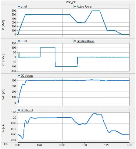
 Firstly, the reference of active power for all three VSC stations ramps up to nominal value of each terminal as indicated in literature [6], while that of reactive power remains zero.

 After it enters the steady state in operation point, the reference settings pair of VSC_C2 varies to several different values as shown in Table 2.10. Here the active power reference changes linearly while the reactive power reference changes in step function. All the other reference values in the two other VSC stations keep unchanged throughout the simulation.

Table 2.10 Reference Value Configuration for VSC_C2 in Load Change Study

Time [s] Pref [p.u.] Qref [p.u.]

0 - 0.1 0->0.5 0 0.1-0.3 0.5 0 0.3-0.5 0.5 0.1 0.5-0.7 0.5 -0.1 0.7-0.8 0.5->0.3 -0.1 0.8-0.9 0.3 0 0.9-1.0 0.3->0.6 0 1.0-1.1 0.6 0 1.1-1.2 0.6->0.1 0 1.2-1.3 0.1 0 1.3-1.4 0.1->0 0 1.4-1.5 0 0

Note here although the rated power of VSC_C2 is 500MW (0.5 p.u.), the case of Pref=600MW is also conducted to set some safety margins in case of control failure. When Pref = 100MW or 300MW, the system is operating at a degraded setpoint. The reactive power reference is usually set as 0 to reduce the current, and thus the loss. Under some circumstances, the OWF might also need to either generate or absorb reactive power from the system. The simulation results of both control and electrical variables in each VSC station are presented in Figure 2.17 and Appendix D. In these figures, the positive direction for active/reactive power is assumed to be from AC grid to VSCs and from VSCs to DC cables, as in Figure 2.10. Based on the result, some conclusions are listed as below:

 The simulation results successfully validate the model and verify the control strategy in nominal operation point and load/production varying scenarios. This is the prerequisite of fault analysis to be introduced in the following chapters.

 During the steady state, the DC current flowing in DC cable is around 1.3kA, which is consistent to the calculated value in Equation (2.18).

Eq. (2.18)

 Since A1 is not controlling the active power, it is responsible for compensating the transmission loss in the system, similar to the slack bus in power flow analysis. According to the measured active power detected at A1, the efficiency of the system at the nominal operational point is around 97%.

(31)

17

 For the described start-up setting, the MTDC system enters steady operational point before 0.3s. Therefore, it is acceptable to simulate the first variation in load at t=0.3s. In the following chapters, the load is assumed constant, but similarly the short circuit fault needs to be implemented after the system enters the stable steady state.

 The active power and reactive power follows the reference value well.

 As VSC_A1 is controlling DC voltage (which usually remains constant), the DC voltage remains almost constant of the nominal value of 400kV throughout the power variation.

 As the DC voltage remains almost constant, DC current will change with the active power. Therefore, it might be tricky for the relays relying on current-signal to distinguish faults from a change in load.

Figure 2.17 Simulation Results of VSC_C2

2.6 Summary and Discussions

This chapter focuses on the modeling of the target VSC-MTDC system in PSCAD. It begins with the system description, specifying the assumptions and simplifications. Then the electrical part of each terminal is introduced component-wise with more details about the sizing, followed by the controlling principle and PI tuning for each controller. Cable configurations are defined by looking up the manufacturer datasheet as well as the data from the literature. To verify the model, a simulation was conducted based on which a series of conclusions are obtained and listed. The model presented in this chapter works as the basis for the remainder of this project in which cable short circuit faults, fault detecting, current limiters and the proposed protection scheme will be implemented.

(32)

18

Chapter 3 DC Cable Short Circuit Study

As mentioned earlier in Chapter 1, VSC-HVDC is very vulnerable to DC faults and requires corresponding protective measures. To better identify fault consequences and protection requirements, the system transient during cable short circuit is studied in this chapter. Literature [3] specifies and defines three stages during the DC cable fault response based on the -equivalent cable model. Taking the distributed parameters and the frequency dependent (phase) cable model into consideration, the travelling wave theory is also introduced in this chapter. After the theoretical analysis, a set of fault scenarios are conducted in PSCAD simulation, based on which some conclusions are drawn. Finally, the chapter ends with summary and discussions.

3.1 Introduction

Unlike conventional HVDC technology where the DC fault current can be successfully suppressed by converters and smoothing reactors, VSCs are highly vulnerable to DC faults, such as DC link short circuits, DC cable short circuits, DC cable ground faults, etc. Among them, cable fault usually occurs more often than in other parts of the system, mainly caused by insulation deterioration or breakdown, electrical stresses, environmental conditions, aging and physical damage [3].

There are three types of cable faults from DC side in a symmetrical monopole cable system:

 Positive line to ground fault

 Negative line to ground fault

 Positive line to negative line fault

Since the system is symmetrical, the first two types can be combined into the same category called DC

cable ground fault, or pole-to-ground fault, while the third called DC cable short circuit or pole-to-pole fault.

DC cable short circuit, though less common than the other type, can cause the most serious problems to VSC. While the IGBT could be blocked for self-protection, the fault current can still flow through the freewheeling diodes, acting as an uncontrolled bridge rectifier [4]. This will be a threat to the diodes, the DC cables as well as the whole MTDC system.

3.2 Fault Response based on Lumped Cable Models

In literature [3], a solid DC cable short circuit fault (Rf=0) in VSC-HVDC system is analyzed in detail where

the cables are simply modeled as the -model equivalent resistance (R) and inductance (L) in series while the grounding capacitors are omitted, as depicted in Figure 3.1 (a). Throughout the response after a pole-to-pole fault occurs, three stages are defined in [3], the equivalent circuit of which are expressed in Figure 3.1 (b):

 Stage 1: capacitor discharge stage, where the DC capacitor get discharged through the fault

 Stage 2: diode freewheel stage, where IGBTs are blocked for self-protection and the freewheeling diodes work as uncontrolled bridge rectifier

 Stage 3: grid current feeding stage, where AC grid feeds the fault via diodes path

Literature [3] further presents the complete fault response divided into the corresponding three stages in Figure 3.2, where the voltage of the capacitor (VC), the current flowing through the DC cable (I_cable), the capacitor (I_C), the VSC station (I_VSI), the diodes (I_D1, I_D2 and I_D3) and the AC grid side (Iga, Igb and Igc) are given. Based on the figure, it is eventually put forward that the second stage is the most challenging stage in protections when the freewheeling diodes are forced to flow an abrupt and devastating overcurrent with high initial value.

(33)

19

Literature [3] also points out that the dc cable short circuit fault response can be featured by two factors:

 Critical time limit (tc), which is the time duration for the DC voltage drops to zero, as t1 in Figure 3.2.  Total freewheel overcurrent value (icable), which is the cable current at the critical time.

Literature [3] further gives the mathematical expressions for the critical time as well as the fault overcurrent throughout the entire process, as presented in Appendix E. With these two factors determined, the action time demand in protection scheme can be determined too. In addition, they can also be used to indicate the fault distance, as shown in Figure 3.3. Therefore, such information could be utilized in relay settings as well.

(a)

(b)

Figure 3.1 Cable Short Circuit Fault Equivalent Circuits for (a) the whole model; (b) each of the three stages (taken from [3])

Stage 1 : Capacitor Discharge Stage

Stage 2: Diode Freewheel Stage

(34)

20

Chapter 3 DC Cable Short Circuit Study

Figure 3.2 Fault Response in VSC DC Cable Short Circuit (taken from [3])

(35)

21

3.3 Travelling Wave Effect

In the previous section, the cable is modeled in lumped parameters as R and L. However, for long submarine cables, it is usually more appropriate to consider the distributed parameters. Therefore, the travelling wave effect needs to be considered, which will be described in this section.

According to the travelling wave theory, the occurrence of a fault triggers a wave to travel along the cable in both directions away from the fault. Once the wave reaches the converter stations at the end of the cable, it will be reflected and refracted according to the reflection and refraction coefficients. Such coefficients are ultimately determined together by the character impedance of the cable and the equivalent impedance of the converter station. For example, if a wave is travelling from the cable (character impedance Z1) to a VSC

station (equivalent impedance Z2), the reflected and refracted voltage and current are given in Equation (3.1) –

(3.4). Thereafter, the reflected wave at the converter station travels back to the faulty point, and once again the similar phenomena of reflection and refraction phenomena occur there.

Eq. (3.1) Eq. (3.2) Eq. (3.3) Eq. (3.4)

Figure 3.4 is a lattice diagram indicating the general idea of voltage wave reflection and refraction in a lossless case with open terminals at each end, where reverse and forward wave denoted as r and f and the reflection coefficients at each converter station as kA and kB [16]. Similarly, the current caused by the DC fault

also travels along the cable with reflections and refractions, so that the step-wise increase will be detected in fault current development. With losses taken into consideration, literature [16] also shows the development of fault current measured at the converter station as in Figure 3.5, where represents the time for the wave to travel from fault to the converter station and kn (n=1,2,…) the damping variable accounting for the attenuation.

Such information will be useful in fault locating which will be introduced in more details in Chapter 4.

(36)

22

Chapter 3 DC Cable Short Circuit Study

Figure 3.5 Fault Current Development at the Converter Station (taken from [16])

3.4 Fault Simulation

Due to the symmetry of the model, the short circuit fault is only simulated in Cable A1C2. To implement the faults with various locations in a handy way, Cable A1C2 is modeled as two segments of d and (200km-d) in length that connected in series, with an extra ‘Fault’ block set in between, as shown in Figure 3.6. The fault is configured as a permanent, solid (Rf=0) pole-to-pole fault occurring at t=1.0s, when the start-up transient has been faded away long before. Moreover, IGBTs will be blocked for self-protection when the cable current exceeds 13kA as indicated in [4].

Figure 3.6 System Overview after Fault Implementation

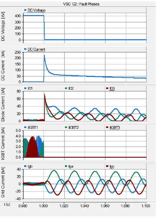
Extensive simulation work has been conducted, which produces a great amount of plots. Only the results of short circuit analysis at VSC_C2 during a fault which is 1km away from VSC_C2 (d=1km) is shwon here as in Figure 3.7. Compared to what is presented in Figure 3.2, the shapes for the measurements look alike. Plus,

(37)

23

the currents flowing through the IGBTs (iIGBT1, iIGBT2 and iIGBT3) are also shown to illustrate the blocking of IGBTs during fault situations.

As can be observed from the figures, the insant when the capacitors are fully discharged (vDC=0, at the

start of 2nd stage), an abrupt overcurrent occurs in diodes, putting them at stake. In this specific case, the critical

time limit is 0.8ms and peak fault overcurrent is around 222kA. This justifies the necessity for DC protection. An

instictive idea will be either to isolate the fault within the critical time limit or to reduce the peak fault

overcurrent with fault current limiters. This validates the theory described in section 3.2 as put forward in [3, 17].

Figure 3.7 DC Cable Short Circuit Study of VSC_C2 (d=1km)

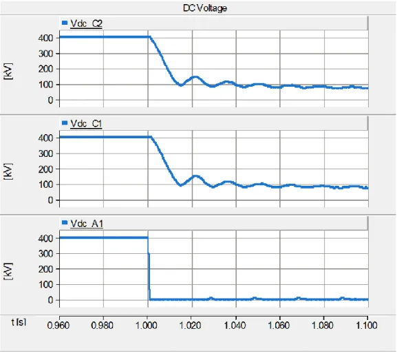
Afterward, DC cable short circuit faults with different distances to VSC_C2 (d) as 1km, 10km, 100km, 190km, 199km are simulated in Cable A1C2 (l= 200km) at t=1s. The results of DC voltage and DC current

(38)

24

Chapter 3 DC Cable Short Circuit Study

detected at VSC_C2 in different sceniros are grouped in Matlab plots, as presented in Figure 3.8. It can be concluded that the closer the fault is to VSC_C2 station, the shorter the critical time and the larger the overcurrent magnitude, thus the more vulnerable the station and the cable connected to it will be. Besides, except for d=1 km or 10km, the DC voltage at VSC_C2 will not drop to 0. In this way, the most severe fault current overshoot is somewhat avoided. Actually, it can be further found out that no distinughishable ‘stages’ can be recognized from the complete fault response in these cases. On the other hand, the critical times for d=1km and 10km are 0.8ms and 2.2ms respectively. Also, when zooming in the fault current upon the fault moment, the travelling wave effect in DC current flowing out of VSC_C2 when d=1km and 10km can also be clearly observed in Figure 3.9, as the current is rising in a stepwise way.

(a)

(b)

Figure 3.8 (a) DC Voltage and (b) DC Current at VSC_C2 during Faults with Different Locations

Figure 3.9 Travelling Wave Effect in DC Current Detected in VSC_C2

1 1.01 1.02 1.03 1.04 1.05 0 100 200 300 400 time [s] D C Volt age [ k V]

DC Voltage with Different Distance to Fault

d=1km d=10km d=100km d=190km d=199km 0.980 1 1.02 1.04 1.06 1.08 1.1 20 40 60 80 100 120

Fault Current with Different Distance to Fault

time [s] D C C urre nt [ k A] d=1km d=10km d=100km d=190km d=199km 1 1 1.0001 1.0001 1.0002 1.0002 1.0003 0 20 40 60 80 100 120 time [s] D C C ure ent [ k A]

DC Current Travelling Wave

d=1km d=10km

(39)

25

Apart from different fault locations, the impacts of various DC capacitance and fault impedance are also studied. Only the conclusion will be provided here: smaller DC capacitance or smaller fault impedance results in shorter critical time and larger overcurrent magnitude, which indicates a more severe situation.

3.5 Summary and Discussions

In this chapter, the DC cable short circuit fault study is illustrated in both theory and simulation. The conclusion indicates that the fault should be cleared before the critical time to protect the system from the

overcurrent. In other words, the key in DC cable short circuit fault protection is to isolate the fault before the

current exceeds the maximum current the components (such as the diodes) can sustain. This means that the DC faults have to be cleared within a few milliseconds, with fault detection, fault localization and fault isolation included [18]. However, such requirements cannot yet fully be satisfied by the existing technology [4, 16]. Therefore, more efficient and reliable fault detecting/locating methods have to be proposed, and fast fault isolation tools need to be designed and tested. Another possible solution is to limit either the magnitude or the derivative of the fault current to a reasonable range by introducing fault current limiters. As a result, the time constraint for the protection system becomes less strict. Each of the possibility will be explored in more details in the chapters to follow.

(40)

26

Chapter 4 Fault Detecting & Locating Principles

As mentioned at the end of the previous chapter, in an attempt to protect the system from overcurrent during a DC cable short circuit fault, three possible directions are put forward:

 Efficient fault detecting and locating principles

 Fast fault isolation devices – DC breakers

 Effective fault current limiting technologies

In this chapter, the first aspect will be discussed while the other two in Chapter 5 and 6 respectively. The chapter introduces both the conventional protecting relays as employed in HVAC as well as more innovative techniques based on the wave transients. Among the large amount of plots generated in the simulations, only the ones in the case when d=10km are selected to represent the principle of each detecting and locating method. Besides, the measured/processed data in different fault scenarios are also summarized in tables for each detecting/locating method.

The simulation time is set as 1.1s while the fault occurs at t=1.0s. The time length is determined based on the assumption that the AC breakers will clear the faults within 100ms even when there is no effective protection from the DC side.

4.1 Introduction

Rapid fault detecting strategy is a prerequisite for the DC protection scheme. It aims to detect if there is a fault, discriminate which is the faulty part, determine which breakers to trip and send them such signals. This is realized by the protection relays.

Fault locating is to estimate the exact fault location in the faulty line. Although this is not compulsory in the protecting scheme, fault locating is still significant and essential in DC cable short circuit since these faults are almost always permanent and require repairs later on. In this circumstances, it is usually assumed that the faulty line has already been determined and isolated from the system. As a result, speed is no longer the highest priority in this condition, and that the data is usually processed offline. However, it is always desirable that the fault location can be estimated only with the data which have already been obtained during the fault.

When it comes to the signal selection, usually both DC current and DC voltage signals can be used. However, in the system studied in this project, the voltage is controlled by VSC_A1. Therefore, the voltage signals cannot distinguish the faulty line from the healthy line when the fault occurs close to VSC_A1, as shown in Figure 4.1 when d=199km. Also, for fault locating, DC voltage signals are not competent either. The DC voltage of VSC_C2 and the DC current flowing out of VSC_C2 during the fault when d= 1km, 10km and 100km are given in Figure 4.2. The figure shows that while the travelling wave effect can be represented in the stepwise increase in the DC current, the DC voltages do not have the similar indications. This can also be verified according to the theory. Since the impedance of the VSC station is assumed to be much less than that of the cable (almost an ideal voltage source), the voltage reflection coefficient is nearly -1. Therefore, the surge will not be clearly visible in the DC voltage at the converter station terminal [19]. Plus, current travelling waves can be extracted by a cost effective design based on a conventional current transformer [20]. As a summary, only the DC current will be the object signals fault detecting and locating in HVDC DC cable short circuit. More specifically, the five currents listed below will be measured; the measurements as well as their positive directions are indicated in Figure 4.3.

 Current flowing out of VSC stations A1 denoted as data A1  Current flowing out of VSC stations C1 denoted as data C1  Current flowing out of VSC stations C2 denoted as data C2

DC Cable Short Circuit Fault Protection in VSC-MTDC

VSC-MTDC

Shining Lu

THESIS REPORT,

DC Cable Short Circuit Fault

Protection in VSC-MTDC

By Shining Lu (4299841)

Abstract

Preface

Contents

Contents

Contents

List of Figures

List of Figures

List of Tables

Abbreviation

Abbreviation

Chapter 1 Introduction

1.1 Background and Motivation

1.2 Problem Description

Chapter 1 Introduction

1.3 Objective and Scope

1.4 PSCAD/EMTDC and Simulation

1.5 Report Layout

Chapter 2 Developing the VSC-MTDC Model

Chapter 2 Developing the VSC-MTDC Model

2.1 System Description

DCS1

DCS2

DCS3

DCS3

Chapter 2 Developing the VSC-MTDC Model

2.2 Electrical Components

Chapter 2 Developing the VSC-MTDC Model

2.3 Control Strategy

Chapter 2 Developing the VSC-MTDC Model

Chapter 2 Developing the VSC-MTDC Model

2.4 Cable Configuration

Chapter 2 Developing the VSC-MTDC Model

2.5 Simulation and Model Validation

2.6 Summary and Discussions

Chapter 3 DC Cable Short Circuit Study

Chapter 3 DC Cable Short Circuit Study

3.1 Introduction

3.2 Fault Response based on Lumped Cable Models

Chapter 3 DC Cable Short Circuit Study

3.3 Travelling Wave Effect

Chapter 3 DC Cable Short Circuit Study

3.4 Fault Simulation

Chapter 3 DC Cable Short Circuit Study

3.5 Summary and Discussions

Chapter 4 Fault Detecting & Locating Principles

Chapter 4 Fault Detecting & Locating Principles

4.1 Introduction