A multiple-goal reinforcement learning method for complex vehicle overtaking maneuvers

vehicle overtaking maneuvers

Author(s)

Ngai, DCK; Yung, NHC

Citation

Ieee Transactions On Intelligent Transportation Systems, 2011,

_{v. 12 n. 2, p. 509-522}

Issued Date

2011

URL

http://hdl.handle.net/10722/137287

A Multiple-Goal Reinforcement Learning Method for

Complex Vehicle Overtaking Maneuvers

Daniel Chi Kit Ngai and Nelson Hon Ching Yung,

Senior Member, IEEE

Abstract—In this paper, we present a learning method to solve the vehicle overtaking problem, which demands a multitude of abilities from the agent to tackle multiple criteria. To handle this problem, we propose to adopt a multiple-goal reinforcement learning (MGRL) framework as the basis of our solution. By con-sidering seven different goals, either Q-learning (QL) or double-action QL is employed to determine double-action decisions based on whether the other vehicles interact with the agent for that par-ticular goal. Furthermore, a fusion function is proposed according to the importance of each goal before arriving to an overall but consistent action decision. This offers a powerful approach for dealing with demanding situations such as overtaking, particu-larly when a number of other vehicles are within the proximity of the agent and are traveling at different and varying speeds. A large number of overtaking cases have been simulated to demonstrate its effectiveness. From the results, it can be concluded that the proposed method is capable of the following: 1) making correct action decisions for overtaking; 2) avoiding collisions with other vehicles; 3) reaching the target at reasonable time; 4) keeping almost steady speed; and 5) maintaining almost steady heading angle. In addition, it should also be noted that the proposed method performs lane keeping well when not overtaking and lane changing effectively when overtaking is in progress.

Index Terms—Artificial intelligence, learning control systems.

I. INTRODUCTION

T

In principle, overtaking is the act of driving around a slower moving leading vehicle in the path of the host vehicle (agent). It can be treated as a three-phase problem [7], which consists of the agent performing the following tasks: 1) diverting from its original lane; 2) driving pass the leading vehicle in the adjacent

Manuscript received March 1, 2008; revised November 24, 2008, September 17, 2009, June 11, 2010, October 12, 2010, and November 2, 2010; accepted December 12, 2010. Date of publication February 7, 2011; date of current version June 6, 2011. This work was supported in part by a grant from the Research Grants Council of the Hong Kong Special Administrative Region, China, under Project HKU7194/06E and in part by the Postgraduate Studentship of the University of Hong Kong. The Associate Editor for this paper was M. Brackstone.

D. C. K. Ngai is with ASM Assembly Automation Ltd., Kwai Chung, Hong Kong (e-mail: [email protected]).

N. H. C. Yung is with the Department of Electrical and Electronic Engi-neering, University of Hong Kong, Pokfulam, Hong Kong (e-mail: nyung@ eee.hku.hk).

Color versions of one or more of the figures in this paper are available online at http://ieeexplore.ieee.org.

Digital Object Identifier 10.1109/TITS.2011.2106158

faster lane; and 3) returning to its original lane afterward. Compared with other AV research, the problem of overtaking has been somewhat neglected. In [7], Shamir proposed an algorithm to compute the optimal trajectory for overtaking a leading vehicle in a straight road. Naranjo et al. [12]–[14] proposed a fuzzy control system that essentially changes the driving mode according to the three phases. Both methods focus on the straight road with one leading vehicle only and are not guaranteed to work if the road has curvature and is occupied by multiple vehicles.

In this paper, we present a learning method to solve the aforementioned vehicle-overtaking problem. We propose to adopt a multiple-goal reinforcement learning (RL) framework as the basis of our solution. RL [15] aims to find an appropriate mapping from situations to actions in which a certain reward is maximized. The vehicle that is responsible for making a decision is called an agent in RL. By considering seven different goals, either Q-learning (QL) or double-action QL (DAQL) [16] is employed for determining action decisions based on whether the other vehicles interact with the agent for that particular goal. QL is a popular RL algorithm, whereas DAQL evolves from QL and uses an autoregressive (AR) prediction model that actively considers the responses of nearby vehicles. While other research concentrates on vehicle control to achieve the goal, the proposed method derives navigation decisions to achieve the same, if not better, results. We believe that vehicle control on throttle, brake, and steering can be easily obtained by the use of proper vehicle dynamic models once correct selection of action to be performed in a particular situation is made. Together with a fusion function, the proposed method offers a powerful approach for dealing with demanding situations such as overtaking. From the simulations, it can be concluded that the proposed method is capable of the following: 1) making correct action decisions for overtaking; 2) avoiding collisions with other vehicles; 3) reaching the target at a reasonable time; 4) keeping a steady speed; and 5) maintaining an almost steady heading angle. In addition, it should also be noted that the proposed method performs lane keeping well when not overtaking and lane changing effectively when overtaking is in progress.

This paper is organized as follows: an overview of the proposed multiple-goal RL (MGRL) framework is given in Section II. Following that, Section III describes the imple-mentation of the RL agent. Section IV presents the details of the method proposed. Section V outlines the simulation environment and the results obtained under different simulation cases. Section VI evaluates the proposed method under different simulation cases. Finally, the conclusion is given in Section VII.

II. MULTIPLE-GOALREINFORCEMENTLEARNING

Depending on the characteristics of the environment, MGRL can be broadly categorized into three types: 1) static known; 2) static unknown; and 3) dynamically changing. A dynami-cally changing environment can be defined as an environment with movable obstacles, and a movable target that their current positions can be detected by the sensors of the agent, but their future movements are not known to the agent. Autonomous road vehicle navigation is an example of applications that act on a dynamically changing environment. In addition, autonomous road vehicle navigation is a multiple-goal problem involving a number of the following tasks at any one time: target seeking, collision avoidance, lane following, lane changing, and safety distance keeping. We believe that this problem can be better solved by solutions that explicitly consider these goals simulta-neously. The MGRL method proposed in this paper is one such solution.

To deal with a dynamically changing environment, it is believed that the motion of the obstacles must be considered. Such consideration must include two aspects: 1) the influence of obstacles’ and/or target’s motion on the agent’s decision-making process and 2) obstacle motion prediction. While there exist methods that adopt the aforementioned view, however, they assume that obstacle motion or behavior is either known asa priori[17], [18] or well defined, e.g., at constant speed and known steering angle [19], [20]. Unfortunately, neither of the assumptions is true in real-world navigation.

Given these limitations, it is motivated in this paper to ex-plicitly consider the “obstacle influence” and “obstacle motion prediction” aspects. In doing so, navigation is no longer treated as a control problem that merely transforms sensor inputs to mechanical outputs. Rather, it is considered as an intelligent decision-making process that deals with higher level strategies called goals with the use of planning, learning, prediction, and the consideration of environment response. Although the goals required in different applications may significantly vary, the navigation problem can now be viewed as a generalized multiple-goal problem. For example, the overtaking problem of the road requires the agent to find a collision-free path while simultaneously obeying the lane following and changing rules. Due to the fact that the road is used by other vehicles that are controlled by other intelligent decision makers (human or otherwise), we need to learn how their decisions will affect the agent’s decision and predict their future actions, before we can appropriately respond in the short term, as well as achieve its goals in the long run. As such, we are motivated to develop a generalized methodology that deals with the multiple-goal requirements in a dynamically changing environment by considering the obstacles’ influence and motion explicitly throughout.

RL is essentially the learning of the mapping of situations (states) to actions. Traditionally, this is done by using the Markov decision process model. However, it describes a single-agent environment in which there is no other decision-making agent in the environment. By viewing the real world as an en-vironment that contains other multiple decision-making agents, it is therefore necessary to consider the decisions made by each

Fig. 1. Conceptual diagram of MGRL.

agent. As such, the double-action concept is introduced to cap-ture this extra piece of information. The DAQL method is thus developed based on this inspiration on top of the foundation of QL. DAQL has explicit consideration on the actions performed (or “influence”) by other parties in the environment and thus allows a more efficient use of the reinforcement leaning method in a dynamically changing environment [21].

Within the context of the proposed method, it is assumed that sensors are employed to capture environmental informa-tion, which is then quantized into discrete states. From these descriptions of the environment, QL or DAQL is used to enable the agent to learn and decide on actions for a particular goal that will bring a maximum reward in the long run, and a goal fusion function is employed to give an overall consistent output action, given that individual actions are derived from individual goals. Eventually, an exploration policy is applied afterward for the RL algorithm to learn through exploring the environment.

Fig. 1 shows the MGRL model with totally G goals, of which conventional QL and DAQL can be picked for learning in any one case, depending on the nature of the environment. Normally, QL is sufficient for cases where there are no envi-ronmental responses or they can be ignored, and DAQL is used otherwise. For example, for a normal navigation problem [22], [23] that consists of two goals, i.e., target seeking and collision avoidance, if other vehicles in the environment or the target is nonstationary, then they have to be dealt with by DAQL, whereas, if they are stationary, then QL will suffice. In the case of vehicle overtaking, we proposed to consider seven goals: 1) target seeking; 2) collision avoidance; 3) lane following; 4) choosing slow lane ifnotovertaking; 5) choosing fast lane if overtaking; 6) keeping steady speed; and 7) keeping steady heading angle. Clearly, some of these goals are contradictory, e.g., goals 5 and 6, whereas some are consistent, e.g., goals 3 and 6. Therefore, a safe and smooth overtaking action requires these goals to be appropriately fused.

Fig. 2. Control variables of agent and theith vehicle.

III. REALIZATION OF THEMULTIPLE-GOAL

REINFORCEMENTLEARNINGAGENT

A. Geometrical Relations Between the Agent and Other Vehicles

1) Quantization of Sensor Inputs: Assume that the envi-ronment consists of one MGRL vehicle (agent) andN other vehicles. The agent is the vehicle that is to perform an over-taking action. The control variables of the agent and the ith vehicle at time t are depicted in Fig. 2. We assume that the vehicle operates in an environment where intervehicle commu-nication is not allowed. It is further assumed that the relative distances between the agent and other vehicles can be sensed by distance sensors on the agent [6], [24]. We further assume that the sensors have a minimum and a maximum detectable distance ofds,minandds,max, respectively. As not all vehicles

are within this range, M vehicles in the environment can be detected, whereM ≤N. Without losing generality, the infor-mation gathered by the agent is quantized into discrete states. In situations where high precision is required, the number of states can be further increased. The location of theith vehicle is denoted by distance di∈Do from the agent, where Do=

[ds,min, ds,max]⊂ , and angleθi∈Θ, whereΘ = [0,2π]⊂

. The two parametersdiandθiare quantized intoNdandNθ

number of discrete states, respectively, as follows:

di = ((Nd−1)×di)/ds,max, ifdi< ds,max Nd−1, otherwise (1) θi = θi+π/Nθ 2π/Nθ , for0≤θi<(2Nθ−1)π/Nθ 0, for(2Nθ−1)π/Nθ≤θi<2π. (2) The state set for vehicle location is defined as si∈Si,

where Si={(di,θi)|di ∈Dq and θi∈Θq1}, Θq1={j |j=

0,1, . . . , Nθ−1}, andDq ={k|k= 0,1, . . . , Nd−1}. There

are altogetherNd×Nθstates forSi. Vehicles are thus located

in a quantized polar coordinate with respect to the agent.

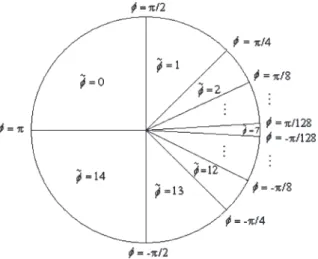
2) Quantization of Sensor Inputs: We assume that the agent’s heading angle isφ∈Θw.r.t. the target. The state set for the relative location of the target is represented by the angleφ∈

Θq2andΘq2={j|j = 0,1, . . . , Nφ−1}, and quantization is

achieved as follows: φ=a if σa+1< φ≤σa (3) where σa= π/2a, fora= 0, . . . , Nφ/2−1 −π/215−a, fora=Nφ/2, . . . , Nφ−1. (4)

Fig. 3. Quantization of heading angleφwhenNφ= 15.

φ is quantized in such a way that there are more states in front of the agent rather than behind it so that the agent can more sensitively respond to vehicles moving in front of it when performing overtaking. Therefore, instead of evenly quantizing

φ,Nφstates are used to quantizeφunevenly, as shown in Fig. 3.

Therefore, we have more states to represent vehicles in front of the agent, because this information is more important to the agent when performing overtaking.

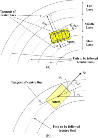
3) Quantization of Lane Information: We assumed that the road has an arbitrary number of lanes while we use a road with three lanes for demonstration in this paper. We further assumed that lane width dlane is derived from lane marking

that can be detected onboard the agent [25]. Furthermore, the center line of the lane and the agent’s relative position to the line can be calculated, as shown in Fig. 4(a). The agent’s location relative to the nearest lane is represented by the perpendicular distance (dLF)between the lane center line

and agent’s center. The difference between its heading angle

(θa,0≤θa≤2π) and the angle of the center line on the

nearest lane (θl,0≤θl≤π) is denoted as θLF, as shown in

Fig. 4(b). dLF and θLF are denoted by dLF∈DLF, where

DLF= [−dlane/2, dlane/2)⊂ , and θLF∈Θ, where Θ =

[0, π]⊂ . The state set for the agent’s location issLF∈SLF,

where SLF={(dLF,θLF)|dLF∈DLF,q and θLF∈ΘLF,q},

ΘLF,q={j |j= 0,1, . . . , NθLF −1}, and DLF,q={k|k=

0,1, . . . , NdLF−1}. We use an equally sized partition to

quan-tize the distance and angle of the agent’s location relative to the center lane. Therefore,NθLF andNdLFdiscrete states are

used to representθLFanddLF, respectively, and quantization is

achieved as follows: dLF= dLF+dlane/2 dlane/NdLF (5) θLF= θLF π/(NθLF−1) . (6)

Furthermore, the perpendicular distance between the agent and the center line of the rightmost or the leftmost lane is denoted bydSLordFL, whereDSL= [−dlane/2,5dlane/2)⊂

Fig. 4. Relation between agent and lane. (a) Distance relation. (b) Angle relation.

the agent’s location with respect to the slow and fast lanes are denoted assSL∈SSL andsFL∈SFL, respectively,

where SSL={(dSL,θLF)|dSL∈DSL,q and θLF∈ΘLF,q},

SFL={(dFL,θLF)|dFL∈DFL,qandθLF∈ΘLF,q},DFL,q =

{k|k= 0,1, . . . ,3NdLF−1}, and DSL,q={k|k= 0,1, . . . ,

3NdLF−1}, and quantization is achieved as follows: dSL= dSL+dlane/2 dlane/(3NdLF−1) (7) dFL= dFL+dlane/2 dlane/(3NdLF−1) . (8)

Since there are NdLF states for the distance between the

agent and the nearest lane, the number of states for the agent in one of the three lanes (fast, middle, and slow) will be three times ofNdLF, i.e.,3NdLF.

4) Actions of the Agent and Other Vehicles: We assume that the agent’s reference heading angle(Δθa)is bounded byθs,max

in each time step. The output actions are therefore given by a∈A, whereA={(|Δva|,Δθa)||

va| ∈CaandΔθa∈Θa},

Ca = {m×ca,max/2|m=−(Nv−1)2, . . . ,(Nv−1)/2},

Θa = {2nθs,max/(Na−1)−θs,max|n= 0,1, . . . , Na−1},

Δva is the change in velocity of the agent, and ca,max is

the maximum acceleration of the agent. We useNv andNa

discrete values to representΔ

va andΔθa, respectively. There

are altogether Nv×Na actions. For DAQL, we assume that

vehicles have velocity|

vo| ∈ + and heading angleθo∈Θ.

They are quantized to a2

i ∈Ao, where Ao={(vo,θo)|vo∈

Fig. 5. General concept of DAQL.

Vqandθo∈Θq3},Vq ={l|l= 0,1, . . . , Nv0−1}, andΘq3=

{j |j = 0,1, . . . , Nθo−1}. Quantization is achieved as

follows: vo= (Nvo−1)× | vo| /vo,max , for0≤vo< vo,max Nvo−1, forvo≥vo,max (9) θo= θo 2π/Nθo (10) where vo,max is the maximum velocity of the vehicle. Since

|

vo|andθoare quantized intoNvoandNθostates, respectively,

there are, altogether, (Nθo−1)×Nvo+ 1 actions for each

vehicle, as observed by the agent. (For |vo|= 0, the vehicle

is at rest, and there is one action only.)

B. Seven RL Goals

By definition, RL is the learning of decision making through the agent’s interaction with the environment. An agent is re-sponsible for the action decision process when it traverses across different environmental states. By making observations of the environment, it captures the current state, which then enables an action decision to be made accordingly. The action results in a reward received to update the value function that guides it to select future actions, which further maximizes future rewards.

QL by Watkins [26] is a simple model-free RL approach that allows the agent to learn to optimally act in the Markovian domain. However, due to its simplicity, it is not very effective in handling a dynamically changing environment, which requires the consideration of actions of other agents/obstacles in the environment [27]. For instance, Team QL [28] considered the actions of all the agents in a team and focused on the fully coop-erative game in which all agents try to maximize a single reward function together. For agents that do not share the same reward function, Claus and Boutilier [29] proposed the use of joint action learners (JALs). JALs learn the value of their own actions in conjunction with those of other agents. Their results showed that, by taking into account the actions of another agent, JALs perform somewhat better than traditional QL. However, JALs crucially depend on the strategy adopted by the other agents and assume that other agents maintain the same strategy throughout, which may not be valid. Hu and Wellman proposed Nash QL [30] that focused on a general sum game that the agents are not necessarily working cooperatively. Nash equilibrium is used for the agent to adopt a strategy that is the best response to

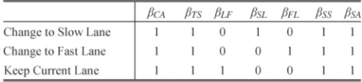
TABLE I

SUMMARY OF THESEVENGOALS

the other’s strategy. This approach requires the agent to learn others’Q-value by assuming that the agent can observe others’ rewards, which is hard in practice. DAQL, as proposed in [23], is an improved version of QL by simultaneously considering the agent’s own action and other agents’ actions. Instead of assuming that the rewards of other agents can be observed, it uses a probabilistic approach to predict their actions so that they may cooperatively, competitively, or independently work. Fig. 5 shows the general concept of DAQL.

1) Collision Avoidance: The function of collision avoidance is to enable the agent to avoid collision with the other vehicles or obstacles. Given multiple mobile vehicles in the environ-ment, DAQL is most applicable here. The DAQL update rule shown in (18) is used to update theQ-values(qi(si,t, a1t, a2i,t))

of eachith vehicle, which represent the action values in differ-ent states qi si,t, a1t, a2t ←qi si,t, a1t, a2t +α rCA,i,t+1+γmax a1 t+1 qi ×si,t+1, a1t+1, a2t+1 −qi si,t, a1t, a2t (18)

wheresi,t andsi,t+1 are the input states,a1t anda1t+1 are the

actions of the agent, and a2

t and a2t+1 are the actions of the

vehicles intandt+ 1, respectively.αandγare the weighting parameter and discount rate, respectively, which both range from 0 to 1. Definedi as the distance between the agent and

theith vehicle at the current time step andd_ias the distance in the previous time step; the reward function adopted by DAQL is defined in (11) in Table I, where T is the sampling time, and therefore, the reward is normalized byva,maxT, where it

is the maximum distance that the agent can travel in one time step. H is a hexagonal area surrounding the agent, as shown in

Fig. 6. H surrounds the agent for the calculation of the reinforcement signal.

Fig. 6, which is defined bydwidth,dlength,df, anddb.dwidth

anddlengthare the width and length of the agent, respectively.

The hexagonal shape allows the agent to move away from other vehicles adopting a linear path apart from a curved path when a circular shape is used.dfis defined by

df =va2/2a+va/2 + 2dlength−vo,i2 /2a (19)

and it is the minimum distance that the agent should keep be-tween a vehicle moving in front of it such that the two vehicles will keep a distance ofdlengthapart if the front vehicle suddenly

stops and the agent responds and brakes after a reaction time of 0.5s.dbis defined similarly in

db=v2o,i/2a+vo,i/2 + 2dlength−va2/2a (20)

but it deals with vehicles behind the agent.

In this case, a negative reward is given either when a collision occurs or when the distance between the agent and other vehicles, which lies inside area H, decreases. WhenrCA,i,tis

available, the agent uses the DAQL update rule to learn collision avoidance with each vehicle in the environment. Given the vehicle’s actions in two time steps [(t−2) and (t−1)], the

agent updates itsQ-values(qi(si,t, a1t, a2i,t))att. Since there

are multiple numbers of vehicles in the environment, we elect to use the parallel QL concept [23], [31], [32], in which allM obstacles share a single set ofQ-values; therefore, theQ-values are updatedM times in one time step.

Apart from learning, the agent also needs to determine its own action in the current time step. Given the state information of the current time step, the agent can use it together with the Q-values to determine an action that is most appropriate for the navigation task. That is, the agent needs to determine an action a1

t, givenqi(si,t, at1, a2i,t). However, sincea2i,tis not known at

t, it has to be predicted, which can be independently treated from RL. To predicta2

i,t, the AR model is adopted. We assume

that accelerations of obstacles are slowly changing in the time intervalTbetween two time steps. A first-order AR model [33], [34] is used to model the accelerationai(t)

ai(t) =Bi,tai(t−1) +e(t) (21)

wheree(t)is the prediction error, andBi,tis a time-dependent

coefficient and is adaptively estimated according to the new distance measurements. The acceleration is thus approximated by a combination of velocity and position representations, i.e.,

ai(t) = 1 T [vi(t)−vi(t−1)] = 1 T2{[ri(t)−ri(t−1)]−[ri(t−1)−ri(t−2)]} = 1 T2[ri(t)−2ri(t−1)−ri(t−2)] (22)

where vi(t)andri(t)are the velocity and position of the ith

vehicle at t, respectively. Substituting (21) into (22) gives a third-order AR model, i.e.,

ri(t)−(2 +Bi,t)ri(t−1) + (2Bi,t+ 1)ri(t−2)

−Bi,tri(t−3) =e(t). (23)

The next position of theith vehicle at (t+ 1) can be predicted by the following equation if the coefficientBi,tis known:

ˆ

ri(t+ 1) =ri(t) +vk(t)T+ ˆBi,tai(t)T2 (24)

whereBˆi,tis time dependent and is updated as follows [35]:

ˆ

Bi,t= Δi,tR−i,t1 (25)

Δi,t=λΔi,t−1+ai(t)aTi(t−1) (26)

Ri,t=λRi,t−1+ai(t−1)aTi (t−1) (27)

where0< λ≤1is a weighting factor close to 1. Sinceai(t),

Δi,t,Ri,t, andλare all known,Bˆi,tcan be predicted, and thus,

ˆ

ri (t+ 1)can be predicted, from which the action performed

by theith vehicle attcan be predicted. Thus, probabilitypa2

i,t

of theith vehicle performing the actiona2_i,tcan be determined. A probability of 1 is given to the predicted action, and 0 is given to all other actions. On the other hand, if the evenly distributed probability model is used,pa2

i,tis equal to1/N0, andN0is the

number of actions observable by the agent. To incorporate the

predicteda2

i,t, the corresponding Q-value can be acquired as

follows: qi si,t, a1t = a2 t p_a2 tqi si,t, a1t, a2i,t . (28)

The expected value of the overall Q-value is obtained by summing the product of the Q-value of the vehicle when it takes actiona2

i,t with its probability of occurrence. Finally, the

summation of theQ-values from all the detected vehicles is the overallQ-value set for the entire vehicle population, i.e.,

QCA a1i = t qi si,t, a1t . (29)

2) Target Seeking: The function of target seeking is to enable the agent to reach the target. The reward function is designed such that the agent receives the maximum reward if it is moving toward the target using the line-of-sight path. For convenience, the target is assumed to be stationary, which suffices for QL. If the target is nonstationary, actions performed by the moving target may be considered as in the case of the vehicle, which the same DAQL formulation applies [22]. We use QL(Q, st, st+1, rt+1)to represent the learning ofQ-value

with the input state stand reward functionrt+1. The general

QL update rule is given as follows: QL(Q, st, st+1, rt+1) :Q st, a1t ←Qst, a1t +α rt+1+γmax a1 t+1 Qst+1, a1t+1 −Qst, a1t . (30)

The QL algorithm applied for target seeking is therefore QL(QTS,φt,φt+1, rDS,t+1), whereφt andφt+1 are the input

states. rTS,t+1 describes the reward received by the agent

generated from the reward function at time t+ 1. We define θT as θT =θa−φ and 0≤θT ≤π. Furthermore, θT is the

angle measured in the current time step, and θ_T is the angle measured in the previous time step. The normalized reward function for target seeking is defined in (12) in Table I, where −1≤rTS,t≤1. The reward function is based on the idea that

higher reward will be given if the agent is moving within line of sight toward the target. The reward proportionally decreases if the vehicle is heading away from the target.

3) Lane Following: The function of lane following is to enable the agent to closely follow the lane. This can be indicated by dLF and θLF. If the agent is properly performing lane

following,dLFandθLFare close to zero. The basic idea behind

then is to minimize the distancedLFand align the agent parallel

to the lane according to the reinforcement signal received. A reward is received if the agent moves toward the center of the lane; otherwise, a punishment is received. Because the lane-following goal is static in nature, QL is sufficient for this purpose.

The QL update rule used in the lane-following goal is QL(QLF, sLF,t, sLF,t+1, rLF,t+1). Define dLF as the distance

in the previous time step, i.e., the reward function that deter-mines the reinforcement signal is defined by (13) in Table I.

A higher reward will be given if the agent is moving tangential to the lane and with a high speed.

4) Changing to Slow Lane and Fast Lane: Different from lane following, lane changing results in decreasingdLFtoward

a specific lane (fast/slow). In this paper, there are two lane-change goals: 1) Change to the slow lane, and 2) lane-change to the fast lane. The fast-lane goal is primarily designed for the agent to overtake from a slow lane using the fast lane but not

vice versa; the slow-lane goal allows the agent to move back to the slow lane after overtaking. QL is used for the agent to learn to achieve the two goals. The QL update rule applied is QL(QSL, sSL,t, sSL,t+1, rSL,t+1)and QL(QFL, sFL,t, sFL,t+1,

rFL,t+1), respectively.

DefinedSLas the distance between the agent and the slow

lane, as shown in Fig. 4(a), and d_SL as the distance in the previous time step; the reward function that determines the reinforcement signal of the slow lane goal is given by (14) in Table I, wherenis the number of lanes in the road.

Similarly, definedFLas the distance between the agent and

the fast lane andd_FLas the distance in the previous time step; the reward function that determines the reinforcement signal of the fast-lane goal is given by (15) in Table I. Therefore, higher reward will be given if the distance between the agent and fast lane is decreasing.

5) Steady Speed: The purpose of the steady-speed goal is to enable the agent to move at the highest available speed while keeping acceleration/deceleration as little as possible. A QL algorithm is assigned to handle the goal and can be described as QL(QSS, sSS,t, sSS,t+1, rSS,t+1), where sSS,t is the state

that refers to the discrete speed of the agent(va)adopted in

the previous time step. Define va as the agent speed in the

current time step and v_a as the speed in the previous time step; the reward function that determines the reinforcement signal is defined by (16) in Table I, whereais the maximum acceleration/deceleration rate of the agent. The reward function is designed such that a reward is assigned to the vehicle if it is accelerating. A penalty is given if it is decelerating.

6) Steady Heading Angle: The purpose of the steady-heading-angle goal is to enable the agent to move with as little change in heading angle as possible. A QL algorithm is assigned to handle the goal and can be described as QL(QSA, sSA,t, sSA,t+1, rSA,t+1), wheresSA,tis the state that

refers to the 15 discrete reference heading angle of the agent

(Δθa)adopted in the previous time step. The reward function

is proportional to the change in heading angle(Δθa−Δθa). A

reward of 1 will be given to the vehicle if the change in heading angle is zero. The reward decreases as the change increases. A reward of 0 is given if the change is equal to the heading angle limit(θs,max), as given by (17) in Table I.

IV. AUTONOMOUSNAVIGATIONAMONG

MOVINGVEHICLES

The proposed MGRL approach considers seven goals in total to solve the overtaking task. To achieve an overall consistence action decision based on the individual action decisions, a goal fusion mechanism is applied to merge the results of the goals. The weighted sum method is used to combine different goals,

Fig. 7. Agent and its nearby regions. TABLE II

DEFINITION OFBFast,jANDBSlowFORLANECHANGING

and three modes are used to adjust the weights. The three navigation modes are given as follows: 1) Change to the slow lane; 2) change to the fast lane; and 3) stay in the current lane. When the change to slow-lane mode is adopted, the agent switches off the lane following and fast-lane goal for it to smoothly move toward slow lane. When the change to fast-lane mode is adopted, the agent switches off fast-lane following and slow lane for it to smoothly move toward fast lane. Finally, when the agent adopted the stay at the current lane mode, the agent switches off slow- and fast-lane mode and stays in the current lane.

To determine which navigation mode to be used, first, we divide the surrounding area of the agent into six regions relative to the agent and aligned with the highway lanes, as shown in Fig. 7. Each region j is assigned with two Boolean values BFast,jandBSlow,j to describe the lane-changing rules in

real-life road networks (see Table II). A “1” means that a change to the fast/slow lane is allowed, and a “0” means that the change is not allowed if there are vehicles in the corresponding region. Changing to slow/fast lane is always allowed if there are no vehicles nearby. We further define bj as a Boolean value, of

which “0” indicates that the vehicles in region j has caused a negative q-value according to the collision avoidance goal

(qi(si,t, a1t))in (28) and “1” otherwise. If there are vehicles

that could cause potential collisions (negative q-value of the collision avoidance goal) in a certain region, then lane changing to that region is not allowed. A rule is designed such that overtaking using the slow lane is not allowed, and therefore, a value of “0” is given to BSlow,5 andBSlow,6. The proposed

method only requires the identification of fast/slow lane and nearby regions with respect to the current lane and, therefore, can be applied to roads with an arbitrary number of lanes.

Therefore, a change to the fast/slow lane is only allowed if the rules in all the regions allow the change, i.e., ifBCForBCS

is true, whereBCF = 6

j=1BFast,j.

The agent then selects to use one of the three modes accord-ing to the followaccord-ing rule. The agent changes to a fast lane ifb5

TABLE III

THREENAVIGATIONMODES ANDCORRESPONDINGVALUES OFβ

is false andBCFis true, and it changes to a slow lane ifBCSis

true; else, it stays at the current lane. Therefore, overtaking will be performed if the agent determined from theQ-value that a collision is expected to happen if it continues to move straight forward and changing to fast lane is safe. Other goals such as collision avoidance are always turned on to make sure that the agent avoids collisions all the time.

Once the mode to be used has been determined, we can combine the Q-values from different goals according to the following method: Qfinal a1_t=QN a1_tW (31)

whereQN(a1t)is a vector of normalizedQ-values from

differ-ent goals, as shown in the following, given that the currdiffer-ent state for each goal is known:

QN a1_t= ⎡ ⎣ QCA a1 t a1 |QCA(a1)| QTS a1 t a1 |QTS(a1)| QLF a1 t a1 |QLF(a1)| × QSL a1 t a1 |QSL(a1)| QFL a1 t a1 |QFL(a1)| QSS a1 t a1 |QSS(a1)| QSA a1 t a1 |QSA(a1)| ⎤ ⎦. (32) Wis the weighting vector containing the weighting param-eters for each goal as given: W= [βCA βTS βLF βSL

βFL βSS βSA]T, whereβ inW are the parameters that vary

between 0 and 1.

In QL or DAQL, eachQ-value reflects the desirability of the agent to perform its associated action. Simply, the larger the Q-value is, the more desirable it is. In the case of a multiple-goal scenario, the Q-values determined from different goals are combined so that the one with the highest combined score carries the most desirable action. In this paper, we employed a weighted summation method to combine the different sets ofQ-values having different weights to illustrate the different importance of these goals.

The three navigation modes allow the agent to adjust the set of weighting parameters (β values) according to the nearby situations. The relation between the three navigation modes and the weighting parameters (β values) is given in Table III. The goal associated with a higher value ofβmeans that it has higher importance when considering the entire task as a whole andvice versa. It should be noted that some of these goals are contradictory to each other, e.g., lane following, slow lane, and fast lane. For instance, when the agent plans to overtake the leading vehicle, it needs to move to a faster lane, whereβSLis

close to 0, andβFLis close to 1.

Once the finalQ-value has been calculated, the final decision of the agent is made by using the ε-greedy policy to allow proper exploration, i.e.,

a1_t = arg max a1 t Qfinal a1 t , with probability1−ε random, with probabilityε.

(33)

V. RESULTS ANDDISCUSSIONS

A. Simulation Environment

In the simulation, we assumed an agent/vehicle dimension of 1.7 m×4.25 m(dwidth×dlength)with a maximum speed

(va,max)of 30 m/s and a maximum acceleration and

deceler-ation of ±3 m/s2. A sensor simulator has been implemented to evaluate distances between the agent and other vehicles. It can produce either accurate or erratic distance measurements fromds,min= 1m tods,max= 100m atT interval (typically

0.1 s) to simulate practical sensor limitations [36], [37]. The lane width in the simulation environment was assumed to be dlane= 3.4m. The other parameters were set as follows:αis

set to 0.6 for faster update ofQ-values;γis set to 0.9 for DAQL and 0.1 for QL; andεis set to 0.2. Without lost of generality, we use the following values for quantizing the states gathered by the agent. In situations where high precision is required, the number of states can be further increased.Nd andNθ are set

to 15 and 16, respectively, for gathering vehicle information. Nφ of 15 is used for quantizing the heading angle.NθLF and

NdLF are set to 16 and 17, respectively, for the gathering of

lane information. Finally, Nv andNa of 5 and 15 are used,

respectively, to represent the action of the agent, whereasNvo

and Nθo of 6 and 16 are used, respectively, to represent the

actions of other vehicles. We use roughly 15–17 partitions for spatial-related parameters and 5–6 partitions for speed-related parameters. More partitions are assigned to spatial-related parameters for better collision avoidance performance. Rela-tively fewer partitions are assigned to speed-related parame-ters to reduce the total number of state.

To learn to solve the overtaking problem, the agent was first trained in a test environment (see Fig. 25) for 1000 episodes. During training, the environment, which consisted of other moving vehicles, changed because of vehicle movements. One episode is defined as either the agent has reached the target (end of the road) or a maximum of 500 steps has been reached, where one time step represents the time interval of T. Explo-ration and learning were enabled during training but disabled afterward. To study the agent’s learning property, we let it alter-natively switch between exploration and no exploration every ten episodes. The average number of collisions per ten episodes is shown in Fig. 8. It shows that collisions mainly occurred in the first 400 episodes. Initially, the number of collision was small, because the agent was also learning other goals such as lane following, which means that the agent does not necessarily follow the lane; therefore, the chance of causing collision was small. Later, the agent learned the ability to follow lanes, and thus, the number of collision increases. After sufficient learning after about 400 episodes, the agent was able to complete rest of the episodes without collisions.

Fig. 8. Learning rate of the agent.

Fig. 9. Original locations of the agent and other vehicles.

Fig. 10. Path and historical locations of the agent and other vehicles.

When applying the theoretical discrete action output on a realistic vehicle, the change in heading angle is smoothened to have more gradual changes to meet the vehicle dynamic.

B. Case 1: Straight Road With Other Vehicles Moving at Constant Speed

With reference to Fig. 9, the agent was originally located at (2.1, 1.7) and traveled at a maximum speed of 30 m/s toward the target at (474, 1.7). There were three straight lanes in the environment, and there were three vehicles. Vehicles 1, 2, and 3 began at (82, 1.7), (141, 5.1), and (82, 8.5) and traveled at constant speeds of 6, 18, and 24 m/s, respectively. The aim of this simulation is to demonstrate how the agent overtakes a slow-moving vehicle. The paths taken by the agent and other three vehicles are shown in Fig. 10. The historical positions of all the vehicles are depicted as red crosses in 1-s intervals.

The simulation result shows that the agent began overtaking aftert≈2s when it was just behind vehicle 1. It moved to the middle and faster lane att≈4s, at which time, it was almost in parallel with and nearest to vehicle 1 and some distance behind vehicle 2. At this point, the agent also commenced the action of returning back to its original lane. At t≈6 s, the agent returned to the slow lane, just ahead of vehicle 1. As vehicle 1 moved slower than the agent, the agent maintained its own speed until the target was reached. This completed the overtaking maneuver without causing a collision or any abrupt changes in speed and heading angle. In these instances, both vehicles 2 and 3 were some distance or lane away and had little impact on the overtaking decision. Throughout the journey, the agent traveled at maximum speed, as shown in Fig. 11. From Fig. 12, it can be seen that the agent started overtaking (a gentle left turn) att= 2.4s and completed the turn att= 4.4s. It then

Fig. 11. Speed profile of the agent.

Fig. 12. Heading angle profile of the agent.

Fig. 13. Path and historical locations of the agent and other vehicles.

began to move back to the slow lane as part of the overtaking action and completed the whole action att= 6.4s.

C. Case 2: Straight Road With Other Vehicles Moving at Variable Speed

In this case, the road configuration is the same as Case 1, except that the three other vehicles were traveling at variable speed that range between 6 and 24 m/s, with acceleration/ deceleration of ±2 m/s2. As shown in Fig. 13, this variable speed per vehicle is depicted as unequal distances traveled between the 2-s intervals. In performing the overtaking action, the agent had to consider the distances of other vehicles in its overtaking path, and in this case, when it first overtook vehicle 1 att= 2.4s, the situation was very similar to Case 1. If vehicle 2 traveled faster or vehicle 1 traveled slower at this point, the agent would probably have returned to the slow lane in its next move. However, vehicle 2 was slowly traveling, and so was vehicle 3; as overtaking from the slow lane is not permitted, it triggered the agent to move to the fast lane att= 7.2 s. At this point, the agent was almost next to vehicle 2, with vehicle 3 some distance behind it in the same lane. As the target was at the end of the slow lane, the target-seeking goal became more important. As a result, it turned right and overtook vehicle 2 before reaching the target. This completed the overtaking maneuver without causing collision or any abrupt changes in speed and heading angle. In this case, it is probable that the agent could slightly slow down and let vehicles 1 and 3 pass first before doing the same thing as shown in Fig. 14 at 3.4 and 7.6 s. From Fig. 15, it can be seen from the heading angle profile that the overtaking began at aboutt= 2.4s, turned left again at t= 7.8s, and commenced a right turn att= 11s.

D. Case 3: Curve Road With Other Vehicles Moving at Variable Speed

In this case, a curved road with three lanes was considered. As shown in Fig. 16, the target at (245, 226) was at the end of

Fig. 14. Speed profile of the agent.

Fig. 15. Heading angle profile of the agent.

Fig. 16. Original locations of the agent and other vehicles.

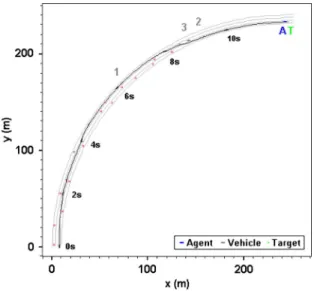
Fig. 17. Path and historical locations of the agent and other vehicles.

the slow lane and the agent, and vehicles 1 (fast lane), 2 (slow lane), and 3 (middle lane) were initially located at (8.5, 0), (1.7, 0), (10, 33), and (14, 69), respectively. The maximum speed of the agent was 30 m/s, whereas vehicles 1, 2, and 3 were traveling at variable speed as in Case 2. Fig. 17 shows

Fig. 18. Speed profile of the agent.

Fig. 19. Heading angle profile of the agent.

the paths of the agent and vehicles and their historical positions in 1-s intervals. As can be seen in Fig. 17, the agent overtook vehicle 2 rather quickly, because it was traveling at relatively low speed. Since the agent was initially located very close to vehicle 2, the agent needed to adjust its speed to ensure there was enough space for it to overtake, thus resulting in the agent slowing down. At about t= 2 s, the agent was in the middle lane, some distance behind vehicle 3 and slightly before vehicle 2 in the slow lane, whereas vehicle 1 was the slowest on the fast lane. As the agent caught up with vehicle 3 at aboutt= 4s, vehicle 2 was almost next to it. Due to collision avoidance and overtaking must be in the fast lane, the agent moved into the fast lane, because vehicle 1 was some distance behind; however, vehicle 3 was too close in front. The agent stayed in the fast lane until roughlyt= 7s, when it was almost next to vehicle 3; it began moving back to the middle lane and slow lane to reach the target at the slow lane. This completed the overtaking maneuver, causing neither a collision nor any abrupt changes in speed and heading angle. From Fig. 18, the agent slowed to avoid running into vehicle 2 initially and did that again when it moved to the fast lane from the middle and moved to the middle lane from the fast lane. From Fig. 19, as the agent has to regularly keep changing its heading angle over the curvature, its angle profile is no longer constant, which is the case here. It appears that the additional lane-changing moves during the overtaking action are evident but not excessive.

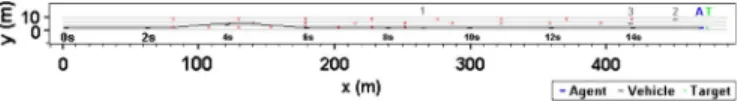
E. Case 4: A Complex Overtaking Maneuver

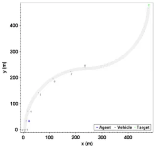
In this case, a more complicated road configuration was used with eight other vehicles involved. Again, these vehicles were traveling at variable speed as in Case 2 and at different initial positions, as shown in Fig. 20. The entire path of the agent and its historical locations are shown in Fig. 21, with the final locations of the other vehicles shown as a reference. From this set of data, four time instants were further investigated, as shown in Fig. 21(a)–(d). Fig. 22 shows the location of the agent with respect to the slow lane.

First, Fig. 21(a) shows the agent’s and other vehicles’ posi-tions att= 7.5s. This was when the agent overtook vehicle 5 by moving from the slow lane to the middle lane. The actual maneuver was about 6.2 s from Fig. 23, and the agent ended up in front of vehicle 4 but behind vehicle 6. Second, Fig. 21(b)

Fig. 20. Original locations of the agent and other vehicles.

Fig. 21. Path and historical locations of agent and other vehicles.

Fig. 22. Location of the agent with respect to the lanes on the road.

shows that the agent completed the overtaking maneuver by moving back to the slow lane, ahead of vehicle 5, att= 11.6s. If vehicle 6 was slower and closer to the agent, it would probably move to the fast lane. It should be noted that, after t= 11.6s, the agent remained in the slow lane untilt= 17s. This was because vehicles 7 (slow lane) and 6 (middle lane) were near each other for a while. At present, the proposed

Fig. 23. Speed profile of the agent.

Fig. 24. Heading angle profile of the agent.

Fig. 25. Evaluation environment.

method is not able to overtake across three lanes; therefore, the agent slowed its speed, as can be seen in Fig. 23, between t= 15−17s and waited for an opportunity.

Third, att= 17s, as shown in Fig. 21(c), the agent detected that vehicles 6 and 7 had sufficient distance between them so that it could overtake them without causing a collision. It should be noted that the agent gradually speeded up to achieve a safe maneuver. Fourth, as shown in Fig. 21(d), att= 22s, the agent completed the maneuver by moving back to the slow lane when the target was reached. Similar to all the cases simulated, the agent completed a series of complex overtaking maneuvering without causing any collisions. The heading angle profile given in Fig. 24 does not indicate any abrupt changes, but the speed profile in Fig. 23 indicates a drop in the agent’s speed due to vehicles 6 and 7 blocking any overtaking actions at the time.

VI. EMPIRICALPERFORMANCEEVALUATION

This section attempts to more specifically evaluate the agent’s performance. The number of vehicles ranges from 0 to 5. Their initial locations are showing in Fig. 25. The maximum speed of the agent was 30 m/s, and other vehicles traveled at variable speed between 6 and 24 m/s. In theory, the shortest path

Fig. 26. Shortest path available. (a) Shortest path. (b) Path following slow lane.

isps= 727m, as shown in Fig. 26(a). On the other hand, the

path following the slow lane is 738 m, as shown in Fig. 26(b). During learning, the agent is placed in an environment that is the same as in Fig. 25, which has five vehicles, and with vehi-cles moving with various speed. To evaluate path performance, the agent performed 1000 episodes in each situation. One episode is defined as the agent reaching the end of the road. The length of the actual path ispa, and the relative error between the

actual path and the shortest path length(pa−ps)/psis denoted

byEr.

To measure the quality of the path adopted by the agent, three indexes are used [34], [38].

1) Safety index (SI)¯c, which represents the percentage of simulation episodes for the simulation task in which the agent successfully reached the target without collision. It is given by

c=m/k (34)

where mis the total simulation episodes without a col-lision, and k represents the total number of simulation episodes.

2) Steering smoothness index (SSI)ω¯, which represents the average absolute value of the heading angle of the agent over the simulation episodes. It is given by

ω= _k i=1 |Δθi| /k (35)

whereΔθistands for the average heading angle in theith

simulation episode. The metric ofωis in radians. 3) Velocity smoothness index (VSI)a¯, which represents the

average value of the velocity change of the agent over the simulation episodes. It is given by

a= _k i=1 |Δvi| /k (36)

whereΔvi stands for the average change of the velocity

in theith simulation episode. The metric ofa¯is expressed in meters per second.

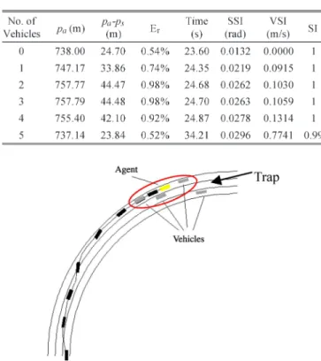
The result of the empirical evaluation on the agent using the evenly distributed probability model is summarized in Table IV.

TABLE IV

PERFORMANCE OF THEAGENTUSING THEEVENLY

DISTRIBUTEDPROBABILITYMODEL

Fig. 27. Formation of “trap.”

The evenly distributed probability model assumes that other ve-hicles have uniform probability of performing different actions. From Table IV, it can be seen that the agent initially adopted a path that is longer than the shortest path as the number of vehicles increases. However, as the number of vehicles is larger than 3, the actual path length decreases. This is because, as there are more and more vehicles on the road, the agent overtakes other vehicles using the fast lane more often, which results in a shorter path. The travel time, SSI, and VSI generally increase as number of vehicles increases. However, when there are five vehicles on the road, the travel time and VSI sharply increase. This is due to the formation of “trap,” as shown in Fig. 27. This resulted in the agent having to abruptly and frequently slow down to avoid collision. Collision may be unavoidable in a “trap” situation if the other vehicles do not adjust their speed accordingly, and the SI in the environment with five obstacles is thus 0.99. However, it should be stressed that such situation will unlikely happen in the real world.

The result of the empirical evaluation on the agent using the AR model is summarized in Table V. When compared with Table III, it can be observed that, although the general result of using the AR model has slightly better path length, travel time, SSI, and VSI than using the evenly distributed probability model [23], the former has a lower SI in the cor-responding situations, which is obviously not desirable. This can be explained as the AR prediction model allows the agent to adopt a more aggressive behavior and carry out collision avoidance behavior only if required. Therefore, the path length can be shorter and smoother. However, if the predicted results are incorrect, it may cause collisions. On the other hand, the

TABLE V

PERFORMANCE OF THEAGENTUSING THEAR MODEL

TABLE VI

ROBUSTNESS TOSENSORNOISE

evenly distributed probability model gives a more conservative prediction, resulting in more conservative actions.

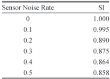
We have also carried out simulation to investigate how the proposed method tolerates inaccuracy in sensor measure-ments. The output of the sensor simulator was deliberately corrupted by a Gaussian noise function that has a mean μ of μ=di and standard deviation σ of n×μ, where n=

0,0.1,0.2,0.3,0.4,0.5, and 0.6 [24] and is called the sensor noise rate. The initial location of the vehicles is the same as in Fig. 25. Vehicles are moving at variable speed, as in the previous case. For each set ofn, the agent was trained for 1000 episodes. After training, the agent was evaluated in the same environment 1000 times with different n’s. Table VI depicts the simulation summary. It shows that the SI decreases by 14.2% forn= 0.5when compared with the environment with no noise.

VII. CONCLUSION

In this paper, we have presented a novel MGRL method that can be used in general for making action decisions in AV navigation. A number of overtaking cases were simulated to demonstrate the effectiveness of the proposed method. By con-sidering seven different goals, either QL or DAQL is employed to determine individual action decisions based on whether the other vehicle interacts with the agent for that particular goal. Furthermore, a fusion function is proposed to weigh the importance of each goal before arriving at a combined but consistent action decision. This offers a powerful approach for dealing with demanding actions such as overtaking, particularly when a number of other vehicles are within the proximity of the agent and are traveling at variable speed. From the results of the four simulation cases, it can be concluded that the proposed method is capable of the following: 1) making correct action decisions for overtaking; 2) avoiding collisions with other vehicles; 3) reaching the target in reasonable time;

4) keeping almost steady speed; and 5) maintaining an almost steady heading angle. In addition, it should also be noted that the proposed method performs lane keeping very well when not overtaking and lane changing effectively when overtaking is in progress. When prediction is concerned, a more conservative approach may be the correct choice. In terms of sensor noise, a larger safety margin should be given to maintain an SI of 1 in all cases.

REFERENCES

[1] A. Broggi,Automatic Vehicle Guidance: The Experience of the ARGO Autonomous Vehicle. Singapore: World Scientific, 1999.

[2] D. Driankov and A. Saffiotti,Fuzzy Logic Techniques for Autonomous Vehicle Navigation. Heidelberg, Germany: Physica-Verlag, 2001. [3] J. P. How, B. Bethke, A. Frank, D. Dale, and J. Vian, “Real-time indoor

autonomous vehicle test environment,”IEEE Control Syst. Mag., vol. 28, no. 2, pp. 51–64, Apr. 2008.

[4] C. Urmson and W. Whittaker, “Self-driving cars and the urban challenge,”

IEEE Intell. Syst., vol. 23, no. 2, pp. 66–68, Mar./Apr. 2008.

[5] J. Feng, J. Ruan, and Y. Li, “Study on intelligent vehicle lane change path planning and control simulation,” inProc. IEEE Int. Conf. Inf. Acquisi-tion, 2006, pp. 683–688.

[6] C. Hatipoglu, U. Ozguner, and K. A. Redmill, “Automated lane change controller design,”IEEE Trans. Intell. Transp. Syst., vol. 4, no. 1, pp. 13– 22, Mar. 2003.

[7] H. Jula, E. B. Kosmatopoulos, and P. A. Ioannou, “Collision avoidance analysis for lane changing and merging,” IEEE Trans. Veh. Technol., vol. 49, no. 6, pp. 2295–2308, Nov. 2000.

[8] A. Kanaris, E. B. Kosmatopoulos, and P. A. Ioannou, “Strategies and spacing requirements for lane changing and merging in automated high-way systems,”IEEE Trans. Veh. Technol., vol. 50, no. 6, pp. 1568–1581, Nov. 2001.

[9] T. Shamir, “How should an autonomous vehicle overtake a slower mov-ing vehicle: Design and analysis of an optimal trajectory,”IEEE Trans. Autom. Control, vol. 49, no. 4, pp. 607–610, Apr. 2004.

[10] F. H. Wang, M. Ying, and R. Q. Yang, “Conflict-probability-estimation-based overtaking for intelligent vehicles,” IEEE Trans. Intell. Transp. Syst., vol. 10, no. 2, pp. 366–370, Jun. 2009.

[11] Y. Zhu, D. Comaniciu, M. Pellkofer, and T. Koehler, “Reliable detection of overtaking vehicles using robust information fusion,”IEEE Trans. Intell. Transp. Syst., vol. 7, no. 4, pp. 401–414, Dec. 2006.

[12] J. E. Naranjo, C. Gonzalez, R. Garcia, T. de Pedro, and M. A. Sotelo, “Using fuzzy logic in automated vehicle control,” IEEE Intell. Syst., vol. 22, no. 1, pp. 36–45, Jan./Feb. 2007.

[13] R. Garcia, T. de Pedro, J. E. Naranjo, J. Reviejo, and C. Gonzalez, “Frontal and lateral control for unmanned vehicles in urban tracks,” inProc. IEEE Intell. Vehicle Symp., 2002, vol. 2, pp. 583–588.

[14] J. E. Naranjo, C. Gonzalez, R. Garcia, and T. de Pedro, “Lane-change fuzzy control in autonomous vehicles for the overtaking maneuver,”IEEE Trans. Intell. Transp. Syst., vol. 9, no. 3, pp. 438–450, Sep. 2008. [15] R. S. Sutton and A. G. Barto,Reinforcement Learning—An Introduction.

Cambridge, MA: MIT Press, 1998.

[16] D. C. K. Ngai and N. H. C. Yung, “Performance evaluation of double action Q-learning in moving obstacle avoidance problem,” inProc. IEEE Int. Conf. Syst., Man, Cybern., Waikoloa, HI, Oct. 2005, pp. 865–870. [17] P. Fiorini and Z. Shiller, “Motion planning in dynamic environments

using velocity obstacles,”Int. J. Robot. Res., vol. 17, no. 7, pp. 760–772, Jul. 1998.

[18] Z. Shiller, F. Large, and S. Sekhavat, “Motion planning in dynamic envi-ronments: Obstacles moving along arbitrary trajectories,” inProc. IEEE Int. Conf. Robot. Autom., 2001, vol. 4, pp. 3716–3721.

[19] C. C. Chang and K. T. Song, “Environment prediction for a mobile robot in a dynamic environment,”IEEE Trans. Robot. Autom., vol. 13, no. 6, pp. 862–872, Dec. 1997.

[20] S. S. Ge and Y. J. Cui, “Dynamic motion planning for mobile robots using potential field method,”Auton. Robots, vol. 13, no. 3, pp. 207–222, Nov. 2002.

[21] D. C. K. Ngai, “Reinforcement-learning-based autonomous vehicle navi-gation in a dynamically changing environment,” Ph.D. dissertation, Dept. Elect. Electron. Eng., Univ. Hong Kong, Hong Kong, 2008.

[22] D. C. K. Ngai and N. H. C. Yung, “Fast-maneuvering target seeking based on double-action Q-learning,” inProc. 5th Int. Conf. MLDM Pattern Recog., Leipzig, Germany, Jul. 18–20, 2007, pp. 653–666.

[23] D. C. K. Ngai and N. H. C. Yung, “Automated vehicle overtaking based on a multiple-goal reinforcement learning framework,” inProc. IEEE ITSC, Seattle, WA, Sep. 2007, pp. 818–823.

[24] C. Ye, N. H. C. Yung, and D. W. Wang, “A fuzzy controller with super-vised learning assisted reinforcement learning algorithm for obstacle avoidance,”IEEE Trans. Syst., Man, Cybern. B, Cybern., vol. 33, no. 1, pp. 17–27, Feb. 2003.

[25] Q. Li, N. N. Zheng, and H. Cheng, “Springrobot: A prototype autonomous vehicle and its algorithms for lane detection,”IEEE Trans. Intell. Transp. Syst., vol. 5, no. 4, pp. 300–308, Dec. 2004.

[26] C. J. C. H. Watkins and P. Dayan, “Technical Note: Q-learning,”Mach. Learn., vol. 8, no. 3, pp. 279–292, May 1992.

[27] M. L. Littman, “Value-function reinforcement learning in Markov games,”Cogn. Syst. Res., vol. 2, no. 1, pp. 55–66, Apr. 2001.

[28] C. Boutilier, “Planning, learning and coordination in multi-agent decision processes,” inProc. 6th Conf. TARK, Renesse, The Netherlands, 1996, pp. 195–201.

[29] C. Claus and C. Boutilier, “The dynamics of reinforcement learning in cooperative multiagent systems,” inProc. 15th Nat. Conf. Artif. Intell., 1998, pp. 746–752.

[30] J. L. Hu and M. P. Wellman, “Nash Q-learning for general-sum stochastic games,”J. Mach. Learn. Res., vol. 4, pp. 1039–1069, Aug. 15, 2004. [31] G. Laurent and E. Piat, “Parallel Q-learning for a block-pushing

problem,” inProc. IEEE/RSJ Int. Conf. Intell. Robots Syst., 2001, vol. 1, pp. 286–291.

[32] G. J. Laurent and E. Piat, “Learning mixed behaviours with parallel Q-learning,” in Proc. IEEE/RSJ Int. Conf. Intell. Robots Syst., 2002, vol. 1, pp. 1002–1007.

[33] N. Kehtarnavaz and S. Li, “A collision-free navigation scheme in the presence of moving obstacles,” inProc. IEEE Int. Conf. Comput. Vis. Pattern Recog., Jun. 1988, pp. 808–813.

[34] C. Ye, “Behavior-based fuzzy navigation of mobile vehicle in unknown and dynamically changing environment,” Ph.D. dissertation, Dept. Elect. Electron. Eng., Univ. Hong Kong, Hong Kong, 1999.

[35] M. J. Shensa, “Recursive least-squares lattice algorithms—A geometrical approach,”IEEE Trans. Autom. Control, vol. AC-26, no. 3, pp. 695–702, Jun. 1981.

[36] C. Hartzstein, “76 GHz radar sensor for second generation ACC,” in

Proc. 11th Int. Symp. ATA EL—New Technologies for Advanced Driver Assistance Systems, Siena, Italy, Oct. 2002.

[37] H. Rohling and M. M. Meinecke, “Waveform design principles for auto-motive radar systems,” inProc. IEEE CIE Int. Conf. Radar, Beijing, China, Oct. 2001, pp. 1–4.

[38] J. Yen and N. Pfluger, “A fuzzy-logic based extension to Payton and Rosenblatts command fusion method for mobile robot navigation,”IEEE Trans. Syst., Man, Cybern., vol. 25, no. 6, pp. 971–978, Jun. 1995.

Daniel Chi Kit Ngaireceived the B.Eng. degree in information engineering and the Ph.D. degree in electrical and electronic engineering from the Uni-versity of Hong Kong, Hong Kong, China, in 2003 and 2008, respectively.

He is currently a Senior Computer Vision Engi-neer with ASM Assembly Automation Ltd., Kwai Chung, Hong Kong. His research interests include artificial intelligence, learning systems, intelligent transportation systems, and computer vision.

Nelson Hon Ching Yung(M’85–SM’96) received the B.Sc. and Ph.D. degrees from the University of Newcastle-Upon-Tyne, Tyne, U.K.

From 1985 to 1990, he was a Lecturer with the University of Newcastle-Upon-Tyne. From 1990 to 1993, he was a Senior Research Scientist with the Department of Defence, Australia. In late 1993, he joined the Department of Electrical and Electronic Engineering, University of Hong Kong (HKU), Pokfulam, Hong Kong, as an Associate Professor. He is the Founding Director of the Laboratory for Intelligent Transportation Systems Research, HKU. He has coauthored six books and book chapters and has published more than 160 journal and con-ference proceeding papers in the areas of digital image processing, parallel algorithms, visual traffic surveillance, autonomous vehicle navigation, and learning algorithms. He acts as an expert in many law enforcement projects and in the courts of law in Hong Kong. He was a Guest Editor for theSPIE Journal of Electronic Imaging. He also serves as a reviewer for a number of IEEE, Institution of Engineering and Technology, and International Society for Optical Engineers journals.

Dr. Yung was member of the Advisory Panel of the Intelligent Transportation Systems (ITS) Strategy Review, Transport Department, HKSAR; Regional Secretary of the IEEE Asia-Pacific region; Council Member and Chairman of Standards Committee of ITS-HK; and Chair of Computer Division, Inter-national Institute for Critical Infrastructures. He is a Chartered Electrical Engineer. He is a member of the Hong Kong Institution of Engineers and the Institution of Electrical Engineers. His biography has been published inWho’s Who in the World(Marquis, USA) since 1998.