A STATE DEPENDENT LANE-CHANGING MODEL FOR URBAN ARTERIALS WITH HIDDEN MARKOV MODEL METHOD
A Thesis by
XIDUO WANG
Submitted to the Office of Graduate and Professional Studies of Texas A&M University
in partial fulfillment of the requirements for the degree of MASTER OF SCIENCE
Chair of Committee, Yunlong Zhang Committee Members, Xiubin Bruce Wang
Clifford Spiegelman Head of Department, Robin Autenrieth
December 2015
Major Subject: Civil Engineering
ii ABSTRACT
The inherent intention and decision process of lane changes are complex and unobservable. Though the external environment and traffic conditions are changing along the traveling direction, the drivers’ characteristics and preferences may lead to persistence of preferable lane choices. Hidden Markov Model (HMM) method is used to model the system that involves unobservable factors, such as speech recognition and biological sequence problems. The hidden process are assumed to associate with observable outcomes.
In this study, HMM is integrated into a two-stage lane-changing model to better represent the mandatory lane-changing behaviors on arterials. The lane-changing decision process is separated into two steps: decision to target a lane as the desire lane and acceptance of available gaps in the chosen direction. The outcome of the first step is unobservable and treated as the latent state in HMM. The second step, gap acceptance model, relates the outcome of the first step to observed vehicle trajectories.
The proposed model is estimated and validated using detail Next Generation Simulation (NGSIM) vehicle trajectory data from Lankershim Boulevard. Comparison between generated lane position sequences and original trajectories validated the model’s capability of representing mandatory lane changes. There is an average 17% difference on predicted lane change locations compared to observed locations; while lane change locations to left turn lane and right turn lane show 10% and 13% difference respectively. The generated lane changes show a late tendency of movements among
iii
through lanes. The results show that the model is fit for the purpose of representing mandatory lane change behaviors on arterials. The research highlights some future improvements of proposed lane-changing model on arterials.
iv DEDICATION
v TABLE OF CONTENTS Page ABSTRACT ...ii DEDICATION ... iv TABLE OF CONTENTS ... v
LIST OF FIGURES ...vii
LIST OF TABLES ... viii
1. INTRODUCTION ... 1
1.1Problem Statement ... 2
1.2 Research Objective ... 3
1.3 Thesis Organization... 4
2. LITERATURE REVIEW ... 5
2.1 Previous Development of Lane Changing Model ... 5
2.2 Hidden Markov Model ... 9
3. MODELING METHODOLOGY ... 13
3.1 Lane Changing Model ... 13
3.2 Likelihood Function ... 19 3.3 Data ... 20 4. MODEL ESTIMATION ... 28 4.1 Estimation Method ... 28 4.2 Estimation Data ... 29 4.3 Estimation Result ... 31 4.4Discussion ... 34 5. MODEL VALIDATION ... 36 5.1 Validation Data ... 37 5.2 Validation ... 39 6. CONCLUSION ... 50
vi
REFERENCES ... 52 APPENDIX ... 55
vii
LIST OF FIGURES
Page
Figure 1 Structure of Toledo’s Lane-changing Model ... 7
Figure 2 Illustration of State Transition of Markov Process ... 10
Figure 3 Illustration of Lane-changing Process ... 14
Figure 4 Hidden State and Observation of HMM ... 18
Figure 5 Lankershim Dataset Collection Site ... 21
Figure 6 Schematic Presentation of Selected Arterial Section ... 22
Figure 7 Schematic Presentation of Sections and Lanes ... 23
Figure 8 Distribution of Lane Changes Location over Sections ... 31
Figure 9 Lane Position of a Vehicle along the Traveling Direction ... 40
Figure 10 Location of Lane Changes along Traveling Direction ... 41
Figure 11 Location Ratio among Lanes ... 44
Figure 12 Percentage of Predicted Lane Changes Occurred Preceding ... 45
Figure 13 Distribution of Lane Change Location from Lane 2 to Lane 1 ... 46
Figure 14 Distribution of Lane Change Location from Lane 3 to Lane 2 ... 46
Figure 15 Distribution of Lane Change Location from Lane 2 to Lane 3 ... 47
Figure 16 Distribution of Lane Change Location from Lane 3 to Lane 4 ... 47
viii
LIST OF TABLES
Page
Table 1 Data Extracted from the Original file ... 25
Table 2 Aggregate Statistics on Different Lanes from Estimation Data ... 30
Table 3 General Estimation Information of Lane-changing Model ... 32
Table 4 Best Solution of Parameters ... 32
Table 5 Definition of Variables in Lane-changing Model ... 33
Table 6 Aggregate Statistics on Different Lanes from Validation Data ... 38
Table 7 Lane Changes Distribution among Sections in Validation Data ... 39
Table 8 Lane Changes Distribution Comparison among Sections ... 42
1
1. INTRODUCTION
Lane changing movement has been regarded as one of the primary driving
behaviors. While the adverse impact of lane changing movements on traffic capacity and traffic safety has drawn a significant amount of research attention in recent past. Lane changing movement has been defined as a driving maneuver that moves a vehicle from one lane to another while both lanes have the same direction of travel. According to Lee et al. (1), the first lateral movement and final straight-ahead point are viewed as the start and end point of lane change maneuvers.
Lane changing models are developed to reflect vehicles’ lateral movements influenced by various external stimulants and individual driving experience; it establish a theoretical framework aim to estimate the probability of lane change movement under certain circumstance. Generally, lane changing models classified the lane change
movements as mandatory lane change (MLC) or discretionary lane change (DLC) based on the stimuli of vehicle maneuvers (2). The discretionary lane changes are mostly made to bypass a slow vehicle and increase traveling speed while the mandatory lane changes usually occur when drivers want to maintain their desire path (3). While lane changing models have been widely used in driving behavior research as a vital component of microscopic traffic simulation, it is important to keep an accurate reproduction of lane changing behavior and its impact on surrounding traffic.
2 1.1Problem Statement
Lane changes are broadly defined as a three-stage decision in most existing models: choice of target lane, decision to accept available gaps and execution of lane change (4). The first two stages in decision process is latent since target lane choice and gap acceptance is unobservable. Drivers make lane changes to keep comfortable driving environment or gain access to desired travel path. The underlying desire of lane changes is influenced by both external and internal factors, as well as the execution process of lane changes. Factors such as geometric condition, surrounding traffic condition, acceleration/deceleration capability of vehicle, and drivers’ experience and preference that involve in the decision process are considered in lane-changing model. These factors are organized and considered with certain lane changes logic, constituting the theoretical framework of the lane-changing models.
In most cases, the changing model considers factors listed above in lane-changing simulation models with addressing the surrounding traffic condition. However, some factors such as drivers’ characteristics have not received adequate attention in existing models. Further, individual preference on lane choice and driving experience may lead to driver persistence of their previous choice. The tendency that adhere to previous choice on lane change decision is concluded as state dependence. Hench, the complexity and randomness of drivers’ decision process behind the observed lane change behaviors need to be investigate, especially for lane changes in congested area. Hidden Markov Model (HMM) is a widely used tool in speech recognition systems and various other
3
areas, which gives the flexibility to model the stochastic lane change behavior with vehicle travel trajectories.
On the other hand, the availability of detailed data of lane change movements is highly related to the accuracy of model. Most traffic simulations compute and update system and vehicle information every time step as well as the corresponding models. Detailed and disaggregate vehicle data are valuable in development and calibration of driver behavior model but not available for most early models. Thus, the complex inherent decision process and the lack of real world traffic data are two main causes for unstable performance of existing lane-changing models.
There is also a need to investigate the difference between freeway analysis and arterial analysis. Most related models were developed based on freeway lane changes. Urban arterial traffic differs from freeway traffic in many respects: signalized
intersection, high proportion of turning movements and shorter headway results in a great amount of lane changes and vehicle interactions. Specific lane-changing model is needed for quality driving behavior simulation on urban arterials.
1.2 Research Objective
This research is aimed to propose a lane-changing model within Hidden Markov Model (HMM) framework for the analysis of lane-changing behavior on urban arterial. For this purpose, the research objectives are:
To introduce the decision process of lane changes and specific factors on urban arterials.
4
To develop an arterial lane-changing model with HMM that capture the influence of the real-time traffic and drivers’ personal traveling preference.
To calibrate the model with real-world traffic data and compare the predicted lane changes with real-world lane change behaviors.
1.3 Thesis Organization
The outline of the thesis, following the introduction, is as follows: previous researches on lane changes model and HMMs method are presented in section 2. The framework of the proposed model and its detail structure are proposed in section 3. This is followed by a general present of arterial dataset used in this study. Then the results of model estimation and validation are listed and summarized in section 4 and 5
respectively. The last section concludes the major findings, limitations and provides suggested direction of further research.
5
2. LITERATURE REVIEW
This section includes previous studies and findings regarding the lane change models, as well as the theory and application of HMM method. Firstly, various
developments on lane-changing model especially microscopic models were introduced. Then it reviews the fundamental knowledge of HMM and some applications in driving behavior modeling.
2.1 Previous Development of Lane Changing Model
From the literature, a considerable amount of work has been present on driving behaviors and traffic simulation applications in latest decades. Several types of lane-changing decision model was presented.
Gipps (2) introduced the first rule-based lane-changing model in 1986, which constrained two intentions of lane change behaviors of vehicles: maintain a desire speed and being in the correct lane to following planned route. The lane-changing algorithm is rule-based: The lane-changing decision process is rule-based: the set of lanes were evaluate respectively and the model checks whether a series of related factors reach fixed conditions, lane changes only execute when all constrains meet the requirement. Factors considered includes safe gap existence, location of permanent obstructions, intended turning movement, presence of heavy vehicles and relative speed. Since the decision process follows predetermined sequence, this model did not consider driver randomness and the latent trade-offs among different factors. Many models have been
6
implemented following Gipps’ concept, including simulation package CORSIM (5), Zhang’s multi-regime model (3), Yang and Koutsopoulos (6) model in MITSIM. Lane changes are separated into MLC and DLC in these models. Concepts of mandatory (MLC) and discretionary lane change (DLC) was clearly classified. As defined in Zhang’s research, MLC occurs when drivers need to connect to next link to maintain their path, bypass a lane blockage downstream, avoid entering a restricted lane and respond to message signs; while DLC in order to increase travelling speed, bypass a slow or heavy vehicle and avoid the lane connected to a ramp. Yang’s model was implemented in MITSIM, which evaluated MLC and DLC respectively with different explanatory factors that helps captured the trade-offs between influential factors for lane changing decision.
A three-stage dynamic discrete choice model was developed for lane-changing maneuvers analysis (3, 7). As mentioned, the three stages of lane changes decision process are as follow: choice of target lane; decision to accept available gaps and execution of lane change. For each vehicle, each lane has its corresponding utilities that represent the attractiveness of keeping or shifting to this lane; relative speed of and desire speed affects lane utilities. Gap acceptance model measures the possibility of lane changes execution. The parameters of MLC and DLC model were calibrated
respectively. Ahmed also pointed out that in heavily congested traffic, the courtesy yielding of lag vehicle enable mandatory lane changes when acceptable gaps are not available.
7
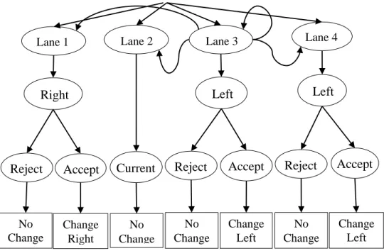
Besides, Toledo’s research (8) adopted similar structure of Ahmed’s model. It integrated MLC and DLC in one utility function that balance the trade-offs between mandatory and discretionary by introducing a variable to represent the relative
importance of mandatory and discretionary. Explanatory variables include neighborhood variables, path plan variables, network experience and driving preference are considered. Figure 1 shows the framework of his discrete choice lane-changing model.
Figure 1 Structure of Toledo’s Lane-changing Model
Moreover, cellular automaton (CA) models and Markov process have been applied in representing the lane changes behaviors in some researches (9, 10, 11, 12, 13, and 14). Lane changing behaviors are considered in multi-lane scenarios in cellular automata models, the incentive and safety criterion need to be satisfy for lane change
Object vehicle Target Lane Immediate Change Gap Acceptance Lane 1
Right Left Left
Reject Current
No Change
Change Right
Lane 2 Lane 3 Lane 4
Accept Reject Accept Reject Accept
Change Left No Change No Change No Change Change Left
8
movements. The unnecessary complexity resulted from cell-structure and some
unrealistic artifacts such as ping-pong phenomenon are two main challenges for CA lane changing models (9, 10). Applications of markov process on lane changes behavior is introduced in next section.
Most studies focused on lane changes behaviors on freeways. Some studies have investigated lane-changing maneuvers on urban arterials and the related characteristics within congested condition (15, 16). Wei et al (17) addressed the influence of path plan on the lane choice decision and the lane change duration in their two-lane arterials lane-changing model. Hidas (18) emphasized the interaction with surrounding vehicles and classified lane changes into three mode: free, forced and cooperative depending on traffic conditions. Sun et al. (19) proposed a model that classified drivers into four types with different background data and driving behaviors, which enhanced the ability to better replicate lane change behaviors and traffic steam in VISSIM.
While many of them facilitated traffic flow studies and simulation, these models were developed for different purposes. Some of them have not been calibrated with real vehicle trajectory records due to of the scarcity of such data; trade-offs among various factors and drivers’ characteristics also contributed to the unstable performance of some existing lane-changing models. Since the relative short duration a driver spends in the mainstream traffic and geometric limitation approaching intersection, the consideration of MLC are expected to rule over other considerations in decision process. Moreover, heavy interactions between vehicles and stochastic driver behavior present challenges for lane-changing modeling.
9 2.2 Hidden Markov Model
Hidden Markov model is a statistical model that models a system with discrete unobservable states as a Markov process (20). A Markov process is a sequence of stochastic state with a finite state set. It is assumed that the system at each time step has its corresponding transition probabilities from current state to next state.
Some studies on lane changes using Markov process were conducted. Pentland and Liu (11) developed a Markov dynamic model for driving behavior includes lane changes. Lane change movement was separated into a series states: starting from centering car position in the current lane; checking available gaps in adjacent lane; initiating lane change; the change itself; steering to complete lane change; and re-centering vehicle position in new lane. The results showed that acceleration and headway pattern defines the driving movement. Singh and Li (12) described the lane change behavior with a Markov chain. In their study, each lane was marked as a state of the process, the state transition probabilities reflected the vehicular movements between lanes.
HMM assumes the latent process that decides the behavior/movement can be measured by analyzing observable outcomes from associated system states. Every future decision is made conditionally dependent on the decision of every previous state; with assumption of initial state, the probability of an event at specific time can be calculated as a joint probability described in the next section. Hence, HMMs have been widely used in modeling sequence problem that involves unobservable factors, such as speech
10
with a set of hidden states by corresponding probability distribution. The HMMs framework endows the model with the ability to handle a sequence of lane-changing behaviors comprised with various factors within finite time.
Figure 2 Illustration of State Transition of Markov Process
Figure 2 shows the state transitions of Markov process. The system can be described as being in one of a set of distinct states {𝑋𝑖} at any time. While the state of a HMM is unobservable, the change of states (or keep in particular state) is undergoes at every discrete time as Markov process. As shown, 𝑋𝑖 is the latent state of modeled
system, and matrix A represents the state transition probabilities that represents the probabilities of move from state i to j (𝐴𝑖𝑗 = 𝑃(𝑋𝑗|𝑋𝑖)). Besides, a HMM is also defined by the following (20):
(1) N represents the number of latent states in the model;
(2) M is the number of distinct observation symbols correspond to the physical output of modeled system.
𝑋1 𝑋2 𝑋4 A12 𝑋3 A21 A34 A43 A13 A31 A24 A 42 A11 A33 A22 A44 A14 A41 A32 A23
11
(3) The initial state distribution π = {𝜋𝑖} gives starting state of observed system,
where 𝜋𝑖 = 𝑃[𝑞1 = 𝑋𝑖], 1 ≤ 𝑖 ≤ 𝑁;
(4) The observation symbol probability distribution in state i, B = {𝑏𝑖(k)}, where1 ≤ 𝑘 ≤ 𝑀.
For a HMM with specification of above components, specific observation sequence can be generate. Hence, λ = (π, A, B) is generally used to indicate a complete HMM system.
There are several applications of HMMs in driving behavior modeling. Zou and Levinson (21) proposed a cluster HMM approach to model driving behavior in conflicts. The driving style in conflicts are recognized as clusters in this model; it is also capable of recognizing driving styles and predicting behaviors based on previous vehicular data. In Kuge et al. (13) research, HMM were used to capture the unobservable internal states of lane changes intentions by connecting latent association with observable variables such as vehicle maneuvers. Toledo and Katz (14) integrating HMM with utility lane-changing model they proposed in their previous work, developed a lane-lane-changing model addressing drivers’ persistence in lane choice. The gap acceptance model connects hidden process and the observable outcome (e.g. vehicle maneuvers), which helps predict lane changes ahead and can be applied to traffic simulation. Not too much work of HMMs have been reported in the field of driving behavior modeling.
It needs to be noted that factors that affect individual lane change behaviors can be classified as geometric conditions, traffic conditions, driver’s driving experience and preference. These factors interact and vary among individuals, and make the prediction
12
of lane changes complex and unreliable. HMMs assume behaviors are series of consecutive stochastic events, which helps deal with the uncertainty of latent decision process.
13
3. MODELING METHODOLOGY
This section presents the methodology for modeling lane change behaviors with vehicle movement trajectory data. Same with some model discussed in previous section (8, 14 and 15), the concept of proposed model is to separate lane-changing movement into two decision steps: target lane choice and gap acceptance, the choice of each step determined the outcome of lane changes. During the decision process, the only
observable action is the lateral movement of vehicle, other decision process such as target lane choice and available gap measure is unobservable. Consideration of this aspect, the proposed model introduces the Hidden Markov Model (HMM) which endows proposed model with ability to measure the latent consecutive decision of lane changes that largely dependent on individual characteristics.
A brief structure of the section is listed as follows: a general framework of proposed lane-changing model is presented. Details on two sub-model of lane-changing process and the Hidden Markov model framework is given. Next two section introduce the likelihood function and dataset used in parameters estimation. Rules and limitation of data processing is illustrated roughly. The dataset used in this study is introduced and processed.
3.1 Lane Changing Model
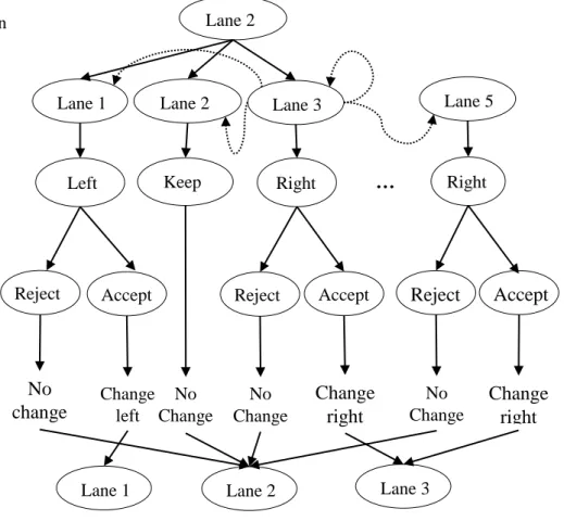
The general framework of proposed lane-changing models is shown in Figure 3. The model involves two sub-model: target lane choice model and gap acceptance model.
14
For the first one, individuals are intend to search all lanes available in the subsequent section and target the lane perceived to be the best in following path. However, the action of vehicle lateral change to target lane may not executed immediately due to the limitation of the road environment and the conflicts with other vehicles.
Figure 3 Illustration of Lane-changing Process
For example, a driver traveling in lane 2 plans to turn right marks lane 5 as the target lane when approaching intersection; the vehicle needs make consecutive lane changes through lane 3, lane 4 then reaches the target lane. Besides, adjacent vehicles may delay driver’s action. The lateral movement of vehicle is the result from several
Current location Target Lane Immediate change direction Gap Acceptance Lane 1
Left Right Right
Reject Keep No change Change left
Lane 2 Lane 3 Lane 5
Accept Reject Accept Reject Accept
Change right No Change No Change No Change Change right Lane 2 Outcome Next location …
15
unobservable decision process, thus, the proposed model is developed on the immediate lane change actions and environment/driver variables related to the decision process.
HMMs are used widely in modeling involves unobservable factors. The observable outcome is associated with a set of hidden states by corresponding
probability distribution. The HMMs framework endows the model with ability to handle a sequence of lane-changing behaviors comprised with various factors within finite time. Details specification of proposed model are presented in following section.
3.1.1 Target Lane Choice Model
Firstly, drivers need to target a lane among all available lanes as the most desirable lane. The attractiveness of each lane is computed by a utility function; many factors would affect the value of the utility function. Variables associated with the desired path, the dynamic traffic conditions, and the driver’s consistency of lane change behavior involve in the utility function.
The utility function for lane i at time t is given below:
𝑈𝑖,𝑡 = 𝛽𝑖𝑋𝑖+ 𝜀𝑖, i ∈ 𝐿𝑛, 𝑡 ∈ 𝑁 (1)
Where,
𝑋𝑖 = explanatory variables that affect the attractive utility of lane i
𝛽𝑖 = corresponding vector of parameters
𝜀𝑖 = random term associate with lane utility for lane i 𝐿𝑛= choice set of available lane
16
Besides, the mandatory lane changes are expected to dominate other considerations such as gaining speed due to the relative short duration that a driver travels in the mainstream. Hence, factors related to keeping desire travel path are considered as most important in the lane choice decision, which include distance to planned exit, the number of lane changes that needs to make to follow driver’s planned path and queue length to the back of queue of in each lane.
The target lane choice probabilities are given by concept of multinomial logit model:
p(TL𝑛,𝑡 = i) =
exp (𝑈𝑖,𝑡)
∑ exp (𝑈𝑗 𝑗,𝑡), i, j ∈ 𝐿𝑛 (2)
Where 𝑇𝐿𝑛,𝑡 is the target lane at time t. The lane with highest utility value will be chosen as the target lane. As mentioned, the relative lateral location between chosen lane and current lane of the vehicle would determine the direction of intended lane change:
If the chosen lane is the current lane, drivers would keep vehicle’s lateral location;
If the chosen lane is on the right side of the current lane, drivers would make a right lateral movement (change right);
If the chosen lane is on the left side of the current lane, drivers would make a left lateral movement (change left);
When the chosen lane is two (or more) lanes away from the current lane, the immediate lane change movement is the same as if the chosen lane is on the right adjacent to the current lane.
17 3.1.2 Critical Gaps Model
The available gaps in this study is measured as the time difference between the preceding and following vehicles in the lane in which subject vehicle is traveling. The model compares the available gap with the critical gap; then, only gaps greater than or equal to the critical gap are accepted by the driver. The critical gap are computed as function of influential factors and individual-specific random term, the function is given as follow:
𝐺𝑛,𝑡𝑐𝑟|𝑣𝑛 = 𝛽𝑛,𝑡𝑋𝑛,𝑡+ 𝜀𝑔 (3)
Where,
𝑋𝑛,𝑡 = explanatory variables that affect the critical gap
𝛽𝑛,𝑡 = corresponding vector of parameters
𝜀𝑔 = random term associate with critical gap, where 𝜀𝑖 ~N(0, 𝜎𝑔2)
Then the probability of accepting available gap is given:
P(𝐺𝑛,𝑡 > 𝐺𝑛,𝑡𝑐𝑟) = P(ln(𝐺𝑛,𝑡) − ln(𝐺𝑛,𝑡𝑐𝑟) |𝑣𝑛) = Φ[ln(𝐺𝑛,𝑡)−(𝛽𝑛,𝑡𝑋𝑛,𝑡+𝛼𝑔𝑣𝑛)
𝜎𝑔 ] (4)
3.1.3 Hidden Markov Model
As stated above, the decision process of lane changes is assumed to have two steps: target lane choice and acceptance of available gap. Within HMMs framework, the result of first step: the chosen target lane, is treated as the latent state; and the second step, gap acceptance model relates the outcome of first step to observed vehicle
18
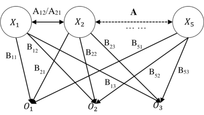
observations (𝑂𝑖), matrix A is the state transition probabilities that represents the
probability of move from latent state i to j (𝑎𝑖𝑗 = 𝑃(𝑋𝑗|𝑋𝑖)), and B is the matrix that contains the probabilities of observing outcome (𝑂1, 𝑂2 𝑜𝑟 𝑂3) when the hidden system state is i, noted as𝑏𝑞𝑖 = 𝑃(𝑂𝑞|𝑋𝑖), q ∈ observation state set. For lane-changing model, the matrix A representing outcome of first step and matrix B can be viewed as results of second step. The observation sequence is the lane position sequence extracted from vehicle trajectories.
Figure 4 Hidden State and Observation of HMM
HMMs assume that the modeled system are consecutive stochastic events, which helps deal with the uncertainty of the latent decision process of lane changes. While, the probability of states at every moment is conditionally dependent on the decision of its previous state; with known initial state, the probability of an event at specific time can be calculated as a joint probability proving in next section.
Hidden State Observation 𝑋1 𝑋2 … … 𝑋5 𝑂1 𝑂2 𝑂3 A12/A21 A B11 B22 B53 B12 B13 B21 B51 B52 B23
19 3.2 Likelihood Function
The probability of available gaps accepted by vehicle n at time t conditional on individual specific characteristics is given by:
𝑃𝑛(𝑙𝑛,𝑡|𝑣𝑛) = 𝑃(𝐺𝑛,𝑡 > 𝐺𝑛,𝑡𝑐𝑟|𝑇𝐿𝑛,𝑡𝑣𝑛) (5)
The probability of individual vehicle n target i as chosen lane at time t conditional on individual specific characteristics is given:
𝑃𝑛(𝑇𝐿𝑛,𝑡= 𝑖|𝑣𝑛) = ∑𝑗∈𝐿𝑛𝑃(𝑇𝐿𝑛,𝑡= 𝑖|𝑇𝐿𝑛,𝑡−1 = 𝑗, 𝑣𝑛)𝑃(𝑇𝐿𝑛,𝑡−1= 𝑗|𝑣𝑛) (6) The joint probability that observe individual vehicle n make lane change from lane j to lane i at time t conditional on individual specific characteristics can be calculated recursively:
P(𝑇𝐿𝑛,𝑡 = 𝑖, 𝑇𝐿𝑛,𝑡−1 = 𝑗|𝑣𝑛) =
𝑃(𝑇𝐿𝑛,𝑡 = 𝑖|𝑇𝐿𝑛,𝑡−1= 𝑗, 𝑣𝑛)P(𝑙𝑛,𝑡|𝑣𝑛)𝑃(𝑇𝐿𝑛,𝑡−1= 𝑗|𝑣𝑛) (7)
where i, j ∈ lane set
Given the initial target lane probabilities𝑃(𝑇𝐿𝑛,1|𝑣𝑛), the probabilities given above can be calculated recursively for any t. The lane changing movement of vehicle n are observed over consecutive time steps T. With the assumption that conditional on 𝑣𝑛
these observations are independent, the joint probability of sequence of observations of individual n is given by formula:
P(𝐼𝑛|𝑣𝑛) = ∏𝑡=1𝑇 ∑ ∑ 𝑃(𝑇𝐿𝑖 𝑗 𝑛,𝑡 = 𝑖, 𝑇𝐿𝑛,𝑡−1 = 𝑗, 𝑙𝑛,𝑡|𝑣𝑛) (8) Where, In represents the sequence of lane change movement outcomes. Given the initial condition 𝑃(𝑇𝐿𝑛,𝑡−1|𝑣𝑛), the joint probability can be calculated recursively using equation 8.
20
With the assumption that observations of different drivers are independent, the log-likelihood function for all N drivers in estimation dataset can be summed up as:
L = ∑𝑁𝑛−1ln (∫ P(𝐼𝑛|𝑣𝑛)) (9)
The parameters of the model would be estimated by maximizing aggregated likelihood function.
3.3 Data
3.3.1 Site Description
The proposed model is based on the assumption that state dependence and time persistence of consecutive lane choice and lane change behavior in urban area. For model estimation and calibration purposes, the dataset should include at least two sections of arterial that allows capturing the effect of desire travel path on lane-changing choice.
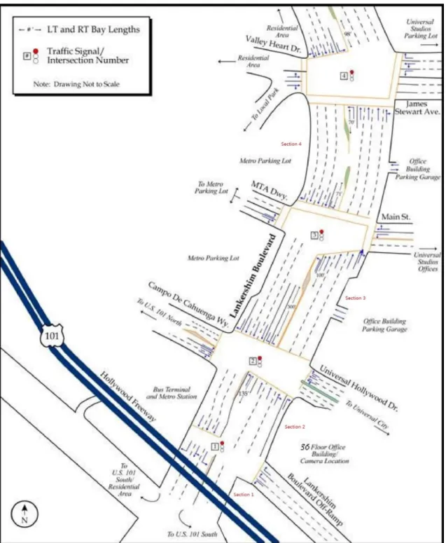
21 Figure 5 Lankershim Dataset Collection Site
Source: Map Data @ 2015 Google
The dataset used to estimate and evaluate model was recorded at Lankershim Boulevard in Los Angeles, California. Figure 5 provides an aerial image of the study area. The data was collected and processed as part of the FHWA’s NGSIM (Next
Generation Simulation) program (22). Lankershim Boulevard is running primarily north-south and selected segment is approximately 1600 feet in length, consists of five sections and four signalized intersections. The source data were collected over 32 minutes from 8:28 a.m. to 9:00 a.m. on June 16, 2005, using five cameras mounted on the roof of a 36-sroty building in the Universal City neighborhood. A schematic illustration of the arterial segment is shown in Figure 6. Details reference indices regards to each section and intersection also listed.
22
Figure 6 Schematic Presentation of Selected Arterial Section
23
The study area covers a typical urban arterials with three to four through lanes on mainline in each direction, and almost every section has exclusive left turning bay approaching the intersection. Turning vehicles make lane change before turning
movements, which provide a great number of mandatory lane-changing movements for model development.
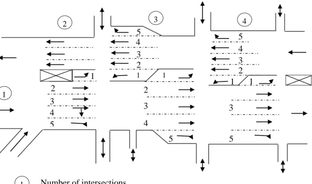
Figure 7 Schematic Presentation of Sections and Lanes
3.3.2 Data Preprocessing
For recording entering and exiting information of each vehicles, only trajectories on section 2, 3 and 4 are used in this studies. Schematic presentation of the selected
1 2 3 4 1 2 3 4 5 3 4 5 2 1 1 2 3 4 5 5 2 1 3 4 3 5 1 Number of intersections 1 2 Number of lanes
24
segment is shown in Figure 7, the reference indices for sections, intersections and lanes are marked respectively.
The half-hour dataset was collected at a rate of 10 frame per second, containing detailed trajectory information such as the vehicle position, lane identification and speed of every vehicle on this section. The dataset have been divide into two periods: one 17-minute period (8:28 a.m. to 8:45 a.m.) for model estimation and one 15-17-minute period (8:45 a.m. to 9:00 a.m.) for model validation. The first one records 705294 observations of total 1211 vehicles while the second one containing 902025 observations of 1231 vehicles.
The raw vehicle trajectory data is detailed in Appendix. To extract vehicle
information for modeling, the original data with given format were transformed to specified structure and more information was extracted using C++. Table 1 presents key information extracted from original dataset.
25 Table 1 Data Extracted from the Original file
Name (Units) Description
Local time (second) Start timing at 8:27:34 a.m., count start at 0 Distance to exit (feet) Distance between the front-center of subject vehicle
and center point of exit intersection
Distance to back of queue (feet)
Distance between the front-center of subject vehicle and the front-center of the last vehicle stopping in
same section
Available gap (second) Available gap in adjacent lane (left and right) of the subject vehicle
Target lane (number) The final target lane of vehicle (1-left turn lane; 5-right turn lane)
Last section length (feet) The length of the last section that subject vehicle traveling on mainline
Remaining distance ratio
(number) The ratio of the distance to exit to last section length Front spacing ratio (number) The ratio of the distance to back of queue to last
section length
For a vehicle traveling north on the road and plans to make a left turn at
intersection 3, the target lane of this vehicle would be 1 and the last section length would be the length of section 3 as 551 feet.
As mentioned above, the available gap of adjacent lane in lane-changing model usually represents by relative lead speed and spacing in front or behind the subject vehicle. Then, the available gap used here is calculated as:
26
where 𝐷𝑓 and 𝐷𝑤are distance between subject vehicle and preceding/following vehicle of adjacent lane,𝑣𝑠 𝑣𝑓and 𝑣𝑤 are velocity of the subject, preceding and following vehicles respectively, 𝑎𝑠 𝑎𝑓and 𝑎𝑤 are velocity of the subject, preceding and following
vehicles respectively, 𝑡𝑠 is the 0.5 second time step used in computation of this study. It
should be noted that surrounding vehicles are defined as the closest vehicle in adjacent lanes within current section. The distance would be negative if surrounding vehicles overlap with the subject vehicle. If the subject vehicle do not interact with any
surrounding vehicle, the distance (𝐷𝑓 and𝐷𝑤) would extend to the boundaries of current section.
The remaining distance ratio and front spacing ratio is proposed to simply the computation in this study. The remaining distance ratio is defined as the ratio of
remaining distance to the length of last section, and the front spacing ratio is defined as the ratio of distance to back of queue to the length of last section. The two ratios were computed using following equation:
𝑟𝑒𝑥= 𝑑𝑖𝑠𝑒𝑥/𝑙𝑠𝑒𝑐 (11)
𝑟𝑞= 𝑑𝑖𝑠𝑞/𝑙𝑠𝑒𝑐 (12)
where 𝑑𝑖𝑠𝑒𝑥 represents the distance to the exit point, 𝑑𝑖𝑠𝑞 is the distance to the back of
queue and 𝑙𝑠𝑒𝑐 is the length of the last section.
Due to the large number of observation records, the raw dataset was filtered based on the following rules:
27
Sampling in the time dimension: the original 0.1 second resolution was converted to a 0.5 second resolution.
Trajectory points outside the mainline section were excluded.
Trajectory points with important missing information were removed.
Except for the 4 rules listed above, further filtering was applied using engineering judgment to remove erroneous trajectory points. From analyzing the coordinates and lane identification for selected sections in the study area, some outlier or erroneous trajectory points were discarded from the analysis.
In summary, this section develops an integrated model for mandatory lane changes on urban arterials within HMM framework. Within HMMs framework, the result of target lane choice model is treated as the latent state; the gap acceptance model relates the unobservable state to observed vehicle trajectories. The proposed model emphasize the desire path factors as well as the consistency of drivers’ lane change behaviors using HMM structure. A brief introduction of detailed vehicle trajectory data used in this study and the pre-processing procedure are given.
28
4. MODEL ESTIMATION
This section presents estimation process of proposed model. The method to maximizing aggregated log-likelihood function mentioned in previous section is descripted first. Then proposed lane-changing model is estimated using the processed estimation dataset. And the estimation results and its discussion is presented below.
4.1 Estimation Method
As illustrated in previous section, for each vehicle, there is a probability that its sequence of movement matched the sequence generated by proposed model. For data used for model estimation, the level of trajectory matches observation sequence can be aggregated into a likelihood function, as noted in section 3.2.
The parameters of proposed model can be estimated by maximizing the
likelihood function used to model the trajectory of the drivers, as mention previously, the calculate equation is given by:
L = ∑𝑁𝑛−1ln (∫ P(𝐼𝑛|𝑣𝑛)) (13)
Related calculating process is given in previous section. The initial hidden and observation states are unobservable, then the starting states of the sequence is also assumed to be dependent on individual specific terms.
In this study, the maximum likelihood estimation is implemented through optim() function provided in statistical software R. The optimization method BFGS algorithm is chosen for its local convergence ability. Due to the fact that the optimization likelihood
29
function is not globally concave, different starting points need to be tested during optimization in order to avoid a local optimal solution.
Hence, an important point noted is that the optimization likelihood function is not globally concave. Due to the individual specific term 𝑣𝑛 is assumed as a normal
distribution, the optimal value of equation 13 may result from different sets of parameters. Different starting points need to be tested during optimization in order to avoid a local optimal solution.
4.2 Estimation Data
4.2.1 General Information
The first 17-minute dataset was used for estimation. Due to the compute limit of parameters estimation, the vehicle trajectory data was randomly sampled at the rate of 1 per every 5 vehicles. The reduced dataset contains 12837 observations of 115 vehicles. The trajectory data of the various drivers in selected segment of arterial and its speeds and accelerations were used to generate required variables.
4.2.2 Data Characteristics
Dataset used for estimation contains 115 vehicles, side street vehicles and vehicles traveling on mainline less than one section were previously excluded. The average trajectory observation duration is 55.81 seconds, with the maximum duration of observation being 133.50 seconds. Out of the 115 observation trajectories, 29 vehicles were (25.2%) traveling northbound and 86 (74.8%) vehicles were traveling southbound
30
on the arterial. Observed vehicles are mostly automobiles (111 out of 115, 96.5%) with only 4 trucks (3.5%) present in dataset. The number of vehicles exited from left turn lane is 68 and the number of vehicles exited from right turn lane is 47.
The aggregate statistic of lane-specific data are given in Table 2. Table 2 Aggregate Statistics on Different Lanes from Estimation Data
Through lane Through & right-turn shared lane Exclusive right-turn lane Exclusive left-turn lane
Average speed (ft./sec) 27.72 26.91 27.46 6.38
Average queue ahead
(number of vehicle) 0.88 0.25 0.17 2.60
Max queue
(number of vehicle) 15 3 3 12
The presence of left turn bay and time conflict between left turn vehicles and opposing through vehicles provides reasonable explanation for the low average speed observed in exclusive left-turn lanes. While speed of right turn vehicles do not affected greatly by the presence of turning bay and its conflicts. The average queue length and maximum queue length values shows that vehicles traveling on right most lane encounter shorter queue at traffic signals compared to through vehicles and left-turn vehicles. The presence of the exclusive turn lanes and its influence on lane-changing behaviors of turning vehicles has been considered in proposed lane-changing model.
There are a total of 147 lane changes observed in trajectory dataset, and the average lane changes is 1.28 lane changes per vehicle in study area; of these, 87 lane
31
changes (59.18%) were made from current lane to left lane and the rest were made to right lane. It should be noted that most of lane changes (110 out of 147, 74.83%) were made after vehicle reaching the last section, while 33 lane changes (22.45%) happened more than one section ahead the exit point and only 8 out 147 (5.44%) occurred two section away; most of these are discretionary lane changes that heading to the opposite direction of vehicles’ target lane. The section distribution of lane changes is given in Figure 8.
Figure 8 Distribution of Lane Changes Location over Sections
4.3 Estimation Result
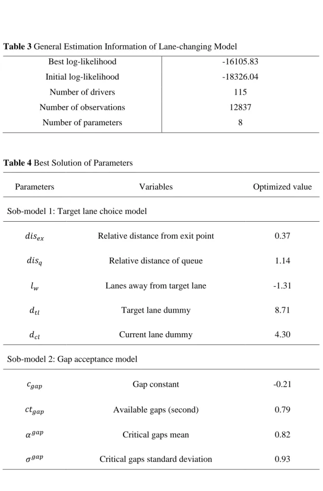
The calculating process and the whole set of parameters are described in previous section. Table 3 presents the summary of estimation results of the proposed model, while Table 4 presents the optimal set of parameters.
0 20 40 60 80 100 120
Section 2 Section 3 Section 4 Outside section N um ber of l ane cha ng es Southbound Northbound
32
Table 3 General Estimation Information of Lane-changing Model
Best log-likelihood -16105.83
Initial log-likelihood -18326.04
Number of drivers 115
Number of observations 12837
Number of parameters 8
Table 4 Best Solution of Parameters
Parameters Variables Optimized value
Sob-model 1: Target lane choice model
𝑑𝑖𝑠𝑒𝑥 Relative distance from exit point 0.37
𝑑𝑖𝑠𝑞 Relative distance of queue 1.14
𝑙𝑤 Lanes away from target lane -1.31
𝑑𝑡𝑙 Target lane dummy 8.71
𝑑𝑐𝑙 Current lane dummy 4.30
Sob-model 2: Gap acceptance model
𝑐𝑔𝑎𝑝 Gap constant -0.21
𝑐𝑡𝑔𝑎𝑝 Available gaps (second) 0.79
𝛼𝑔𝑎𝑝 Critical gaps mean 0.82
33 The definition of variable is given in Table 5. Table 5 Definition of Variables in Lane-changing Model
Variables name Definition
Relative distance from exit point The longitudinal distance remaining to reach the planned exit of vehicle
Lanes away from target lane Number of lane changes needs to make to reach planed target lane
Relative distance of queue The longitudinal distance to last front vehicle stops in lanes
Target lane dummy 1 if the lane is the planned target lane of vehicle, 0 otherwise
Current lane dummy 1 if the lane is the current lane of vehicle, 0 otherwise
Gap constant Constant in mean of lead critical gap function Available gaps (second) Available time gaps between preceding and
following vehicles in adjacent lane (left/ right) mean Heterogeneity term of mean of critical gap Critical gaps standard deviation Standard deviation of critical gap
Given the optimized parameters, the proposed model can be expressed as follows:
𝑈𝑖,𝑡 = 0.37𝑑𝑖𝑠𝑒𝑥−1𝑙𝑤 − 1.31𝑙𝑤 + 1.14𝑑𝑖𝑠𝑞+ 8.71𝑑𝑡𝑙+ 4.30𝑑𝑐𝑙+ 𝜀𝑖𝑛 (14)
where, 𝑈𝑖,𝑡 is the utility of lane i at time t and 𝜀𝑖𝑛represents the generic random term associated with lanes utility. For variables of other parameter terms in above equation, refer to Table 4.
34
And the gap acceptance model can be presented as follow:
𝐺𝑛,𝑡𝑐𝑟 = exp [0.21 + 0.79𝑐𝑡
𝑔𝑎𝑝− 0.82𝑣𝑛 + 𝜀𝑔,𝑛𝑡] (15)
where 𝐺𝑛,𝑡𝑐𝑟 is the critical gaps for lane changes behaviors, 𝑐𝑡𝑔𝑎𝑝 represents available gaps
surrounding subject vehicles and 𝜀𝑔,𝑛𝑡~N(0, 0.932).
4.4Discussion
The estimated parameters help predict the drivers’ desirable lane at every time interval during the entire period traveling on the mainline. As expected, the results indicate that drivers’ intention to travel in the target lane increases with the decrease of distance to the planned exit; the aggressiveness of lane change to the target lane is much larger when more than one lane change movement is needed. The current lane dummy and target lane dummy captures the driving tendency of keeping lateral location and following desire travel path respectively; the relative large value of these two variables reflect drivers’ strong preference to avoid unnecessary lateral movement on arterials (for example, a change to left while the target lane is on the right). The parameter of distance to back of queue captures the influence of intersections and signals. The result that lanes with short queue ahead having larger utility values indicates drivers’ tendency to avoid waiting in queue. The critical gap increases with the available gap. The critical gaps values fluctuated, with a lower limit value around 2 seconds.
The estimation method, data and results of proposed model are present in this section. With the maximization of likelihood function, parameters of a set of variables are optimized; the results of parameters are consistent with the original hypothesis on
35
lane selection process. Next section will presents the validation process set to attempt to evaluate the ability of proposed model to forecast lane change behaviors.
36
5. MODEL VALIDATION
In this section, the predicted lane changes movements from proposed model are compared against the real vehicle lane changes movements for validity. The general procedure of comparison includes:
Extracting lane changes information such as location and direction from vehicle trajectories,
Generating predicted lane position sequence using the proposed lane-changing model
In the validation process, the trajectory data from the 15-minute dataset collected from the same site was used for forecasting lane change behaviors. The reduced vehicle trajectory dataset for validation contains 55253 observations of 433 vehicles, with all vehicles traveling on mainline of selected segment of arterial. Information such as vehicle speed and acceleration is extracted and used to generate aggregate statistics of the original data. Same with the estimation process, the validation is implemented through scripts written in statistical software R. Comparisons were made between the outcome from the proposed model and lane change movements recorded in dataset. The dataset used, and the validation process and results are presents below.
37 5.1 Validation Data
5.1.1 General Information
The second 15-minute dataset is used for model validation. After randomly sampling, the reduced vehicle trajectory data contains 55253 observations of 433 vehicles, all vehicles traveling on mainline of selected segment of arterial. Information such as vehicle speeds and accelerations is extracted and used to generate aggregate statistics of original data.
5.1.2 Data Characteristics
The first 17-minute dataset was used for estimation. Due to the compute limit of parameters estimation, the vehicle trajectory data was randomly sampled at the rate of 1 per every 5 vehicles. The reduced dataset contains 12837 observations of 115 vehicles.
Dataset used for validation contains 433 vehicles, the average trajectory
observation duration is 63.80 seconds, and the vehicle with longest observations during was recorded for 175.0 seconds. Out of the 433 observation trajectories, 172 vehicles (39.7%) traveling northbound and 261 (60.3%) vehicles traveling southbound on the arterial. Observed vehicles are mostly automobiles (427 out of 433, 98.6%) with only 6 trucks (1.4%) present in dataset. The number of vehicles exited from left turn lane is 241, reaches a higher proportion (55.7%) than vehicles exited from right turn lane (192 vehicles, 44.3%).
38
Table 6 Aggregate Statistics on Different Lanes from Validation Data
Lane 1 Lane 2 Lane 3 Lane 4 Lane 5 Average speed (ft./sec) 6.34 13.35 26.11 17.84 13.36
Average queue ahead (number of vehicle)
2.11 2.94 0.87 2.41 0.67
Max queue (number of vehicle) 15 17 9 11 6
The aggregate statistic shows a big difference among lanes: the slower speed and longer queue on the left/right most lane and its adjacent lane is result from high volume of turning vehicle, which account for 30.2% of total volume. Due to the geometric limitation of turning bay (lane 1 and lane 5), the accumulated queue for turning has been transfer to adjacent through lane, with an average queue longer than two vehicles. While vehicles traveling on lane 3 encountered much shorter queue.
There are a total of 683 lane changes observed in trajectory dataset, and the average number of lane changes is 1.58 per vehicle in this study area; of these, 301 lane changes (44.07%) were made from the current lane to left lanes and the rest were made to right lanes. It should be noted that most of lane changes (577 out of 683, 84.48%) were made after vehicle reaching the last section, out of these 95 lane changes occurred more than one section ahead the exit point and the rest two sections away.
39
Table 7 Lane Changes Distribution among Sections in Validation Data
Northbound Southbound All directions
Section 2 153 2 155 Section 3 80 280 360 Section 4 60 84 144 Outside 18 6 24 Total 311 372 683 Number of vehicles 172 261 5.2 Validation
In order to test proposed model, scripts written in R is used to implement the prediction of lane change behavior among observation period, with vehicle information and environment data extracted from original validation dataset. The probability of vehicle lane position are calculated every 0.5 second. And the predicted lane change point are determined by the time that the lane with the largest probability changed from previous time point. The validation process of traffic model establishes its validity by testing and comparing lane changes statistics obtained from proposed model and from the summaries of trajectory data presented in previous section, discretionary lane changes in original dataset is excluded as its behavior have not been emphasized in proposed model.
40 5.2.1 Result
For every vehicle trajectory in the validation dataset, a corresponding predicted lane position sequence is generated. The following figure (Figure 9) shows the lane position outcome from the proposed lane change model for a single right turn vehicle (vehicle id: 77). As shown in figure, the horizontal axis indicates the distance to exit point, and the vertical axis presents the lateral position of lanes along the traveling direction. It presents lateral position of vehicle and location of its lane changes; the predict location from lane 3 to lane 4 is about 30 feet precede to the observed point while the location to the right most lane is a little behind.
Figure 9 Lane Position of a Vehicle along the Traveling Direction
1 2 3 4 5 Lane Ident if ica ti on Remaining distance
41
Figure 10 Location of Lane Changes along Traveling Direction
The generated lane position sequence is compared to its corresponding lane change location of trajectory data, which was extracted and presented in previous section. The locations of lane change simulated by proposed model and extracted from trajectories is compared in Figure 10. As presented, the distribution of predicted lane change location is accord with the trajectory data. The observed lane change locations are more concentrate to certain segment of the road, while the predict lane change points
0 10 20 30 40 50 60 70 80 0 0 . 1 0 . 2 0 . 3 0 . 4 0 . 5 0 . 6 0 . 7 NU M BER OF L A NE CHA NG ES
LANE CHANGE LOCATION: DISTANCE TO EXIT (FEET)
HUNDREDS
42
show a close tendency to exit: no lane changes is made 500 feet away from vehicles exit point.
Table 8 Lane Changes Distribution Comparison among Sections
Total In section 2 In section 3 In section 4 Outside the section
Observed 683 157 359 144 23
Mandatory
observed 597 150 332 94 21
Predicted 597 144 340 110 5
Table 8 presents the distribution of predicted mandatory lane changes and those from the observation from the trajectory data. Each vehicles makes an average of 1.58 lane changes while traveling the whole section in the data and the predicted value from the model is 1.38 lane changes. There are 554 predicted lane changes, comparing to the actual observed lane changes of 683. The slightly low number of lane changes is due to the fact that our model is a mandatary lane change model that heavily penalizes lance changes away from the target lane. Such discretionary lane changes do happen in in the real-world but is not accounted for because the focus of our model is mandatary lane changing. The results indicate that overall the predicted lane change locations (in terms of sections) match well with the observed locations. It needs to be noted that the predicted lane change point are determined by the probability that the subject vehicle travels in certain lane.
The ratio of observed lane change location to predicted lane change location 𝑟𝑐 is proposed as:
43
𝑟𝑐 = 𝑟𝑙𝑐/𝑟𝑝𝑙𝑐 (16)
where 𝑟𝑙𝑐 is the distance ratio of the observed lane change point, and 𝑟𝑝𝑙𝑐 represents the distance ratio of the predict lane change point. The location ratio is used here to identify relative lane change locations simulated by proposed model to observation data. Table 9 presents the location ratio among 5 lane change scenarios.
Table 9 Location Ratio among Lanes
Lateral movement direction Ratio Number of lane
changes
Change to left From lane 3 to lane 2 1.91 30
From lane 2 to lane 1 0.90 239
Change to right
From lane 2 to lane 3 2.06 20
From lane 3 to lane 4 1.79 125
From lane 4 to lane 5 0.87 184
44 Figure 11 Location Ratio among Lanes
As shown in Figure 11, the location ratio of predicted lane changes among all direction is 1.17, which indicates the predicted lane change location precedes to the observed location, especially for lane changes between through lanes (lane 2 through 4). However, the lane change location to turning lane (lane 1 and lane 5) only slightly behind the actual location observed in trajectory data.
Figure 12 presents the percentage of predicted lane changes occurred preceding to the observed location. Most of lane changes among through lanes are behind its observation location (for lane changes from lane 3 to lane 2, from lane 2 to lane 3 and from lane 3 to lane 4 is 13.3%, 15.0% and 20% respectively). Thus, the prediction of lane changes to turning lane is more reliable compared to lane changes between through lanes. 0 0.5 1 1.5 2 2.5 ln 3 to ln 2 ln 2 to ln 1 ln 2 to ln 3 ln 3 to ln 4 ln 4 to ln 5 Average L oc ati on ra ti o
45
Figure 12 Percentage of Predicted Lane Changes Occurred Preceding
The distributions of lane change locations and its cumulative percentage of the three lane change movements are presented in Figure 13-17. Heavy lane change
locations are identified if lane changes concentrate on a specific segments of the arterial. By comparing two distribution curves for lane changes from lane 2 to lane 1 (Figure 13), the observed and predicted cumulative curves match well, with more mandatory lane changes predicted closer to the exit point. Figure 14 presents the distribution from lane 3 to lane 2. 0.00% 10.00% 20.00% 30.00% 40.00% 50.00% 60.00% 70.00% 80.00% ln 3 to ln 2 ln 2 to ln 1 ln 2 to ln 3 ln 3 to ln 4 ln 4 to ln 5 P erc entag e of total obse rva ti on
46
Figure 13 Distribution of Lane Change Locationfrom Lane 2 to Lane 1
Figure 14 Distribution of Lane Change Locationfrom Lane 3 to Lane 2
0.00% 10.00% 20.00% 30.00% 40.00% 50.00% 60.00% 70.00% 80.00% 90.00% 100.00% 0 10 20 30 40 50 60 70 0 0 . 1 0 . 2 0 . 3 0 . 4 0 . 5 0 . 6 C U MUL A TI V E P R EC EN T L A N E C H A N G ES O C C U R R ED N U MBE R O F L A N E C H A N G ES
LANE CHANGE LOCATION: DISTANCE TO EXIT (FEET)
HUNDREDS
observed predict observed cumulative predict cumulative
0.00% 10.00% 20.00% 30.00% 40.00% 50.00% 60.00% 70.00% 80.00% 90.00% 100.00% 0 1 2 3 4 5 6 0 . 0 0 0 . 0 2 0 . 0 4 0 . 0 6 0 . 0 8 0 . 1 0 0 . 1 2 0 . 1 4 0 . 1 6 0 . 1 8 0 . 2 0 C U MUL A TI V E P R EC EN T L A N E C H A N G ES O C C U R R ED N U MBE R O F L A N E C H A N G ES
LANE CHANGE LOCATION: DISTANCE TO EXIT (FEET)
47
Figure 15 Distribution of Lane Change Locationfrom Lane 2 to Lane 3
Figure 16 Distribution of Lane Change Locationfrom Lane 3 to Lane 4
0.00% 10.00% 20.00% 30.00% 40.00% 50.00% 60.00% 70.00% 80.00% 90.00% 100.00% 0 1 2 3 4 5 6 7 8 0 0 . 0 2 0 . 0 4 0 . 0 6 0 . 0 8 0 . 1 0 . 1 2 0 . 1 4 0 . 1 6 0 . 1 8 0 . 2 0 . 2 2 CU M U L A TI V E P RE CE N T L A N E C H A N G ES O C C U R R ED N U MBE R O F L A N E C H A N G ES
LANE CHANGE LOCATION: DISTANCE TO EXIT (FEET)
HUNDREDS
observed predict observed cumulative predict cumulative
0.00% 10.00% 20.00% 30.00% 40.00% 50.00% 60.00% 70.00% 80.00% 90.00% 100.00% 0 5 10 15 20 25 30 0 . 0 0 0 . 0 5 0 . 1 0 0 . 1 5 0 . 2 0 0 . 2 5 0 . 3 0 C U MUL A TI V E P R EC EN T L A N E C H A N G E S O C C U R R E D N U MBE R O F L A N E C H A N G ES
LANE CHANGE LOCATION: DISTANCE TO EXIT (FEET)
HUNDREDS
48
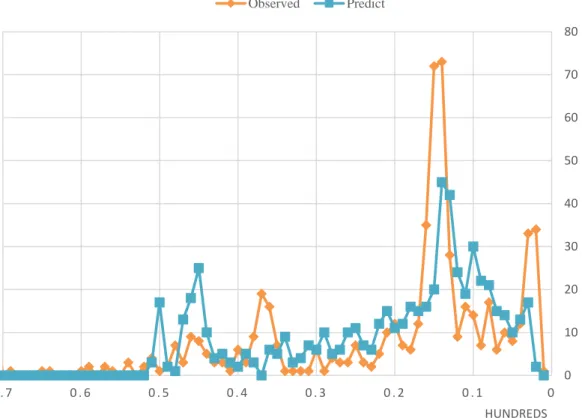
Figure 17 Distribution of Lane Change Location from Lane 4 to Lane 5
Moreover, aggregated location of lane changes can be observed in Figure 15 and 16 represents lane changes from lane 2 to lane 3 and lane 3 to lane 4 respectively. For lane changes from lane 3 to lane 4, the observed distribution shows two aggregate sections that located respectively at 180 and 400 feet precede to the intersection. However, 75% of predicted lane changes were made at a 150-feet section peak at 200 feet before exit. Lane changes among lane 2 and lane 3 distributed among traveling segment and tend not accumulative a certain section. Thus, the predicted outcomes are not in accord with observed lane changes.
For lane changes into the right-turning lane (from lane 4 to lane 5, presents in Figure 17), it can also be noted that the predicted mandatory lane changes tend to
0.00% 10.00% 20.00% 30.00% 40.00% 50.00% 60.00% 70.00% 80.00% 90.00% 100.00% 0 5 10 15 20 25 30 35 40 45 50 0 . 0 0 0 . 0 5 0 . 1 0 0 . 1 5 0 . 2 0 0 . 2 5 CU M U L A TI V E P RE CE N T L A N E CH A N G E S O C C U R R E D N U MBE R O F L A N E C H A N G ES
LANE CHANGE LOCATION: DISTANCE TO EXIT (FEET) HUNDREDS
49
concentrate towards the exit point. The results also shows that the predicted lane change point of right turn vehicle is not as precise as predictions for the left turn lane, which may be resulted from the geometric limitation of the exclusive turning bay. For lane changes from lane 4 to lane 5 in section 3 (exclusive turning bay available in both
direction), the location ratio reaches 0.90, but this ratio is not as good when the exclusive right turning lane is not available. The interaction with through vehicles on shared through and right turn lanes likely have contributed to this inconsistency.
The validation of proposed lane-changing model is presented in this section. The comparison of the lane change location ratio and location distribution of different movement directions were discussed. The results suggest that the model is fit for the purpose of representing mandatory lane change behaviors on arterials.
50
6. CONCLUSION
This study develops a mandatory lane-changing model for urban arterials with HMM method. The decision process of lane changes is separated into two steps: lane choice and acceptance of available gaps. With the integration of the two steps into a HMM framework, the lane-changing model offers the prediction of lane identifications that emphasized the state dependence. The result of first step, target lane choice, is modeled as the latent state in HMM because the choice is unobservable. The second step, gap acceptance model relates the lane choice to observable vehicle trajectories. After identification of influential variables and parameters estimation, the proposed model is capable of generating lane position predictions and presenting lane changes locations.
With the integration of two steps, the decisions of lane changes is assumed to determine by outcomes of two sub-mode; in addition, the HMM method emphasizing the state dependence of previous choices. Thus, the integrated lane-changing model offers the prediction of lane changes behaviors. The result of first step, target lane choice, is modeled as the latent state in HMM because the choice is unobservable. The second step, gap acceptance model related the lane choice to observable vehicle trajectories. After identification of influential variables and parameters estimation, the predictions of lane changes behavior are presented.
The results of validation show an average 17% difference on location of lane changes when compared with real vehicle trajectory. And lane change locations to left
51
turn lane and right turn lane show 10% and 13% difference respectively. The generated lane changes show a late tendency of movements among through lanes. However, the location results should still be within a reasonable range of sections.
There is still work to be done on this topic in the future. Future improvements of this research may include: deploying the proposed model in microscopic traffic
simulation and comparing MOEs obtained from simulated traffics, checking the
applicability of proposed model to different traffic scenarios if other suitable datasets are available. Additionally, it would be interesting and challenging to consider more factors such as vehicle classes and its acceleration ability. With considering more variables and balancing trade-offs between discretionary lane changes and mandatory lane changes, the future model might be able to representing the lane change behaviors in various traffic scenarios.
52 REFERENCES
1. Lee, S. E., Olsen, E. C., and Wierwille, W. W. A comprehensive examination of naturalistic lane-changes. DOT HS-809 702. U.S. Department of Transportation, 2004.
2. Gipps, P. G. A model for the structure of lane-changing decisions. Transportation Research Part B: Methodological, Vol. 20, 1986, pp. 403-414. 3. Zhang, Y., Owen, L. E., and Clark, J. E. Multiregime approach for microscopic
traffic simulation. In Transportation Research Record: Journal of the Transportation Research Board, No. 1644, Transportation Research Board of the National Academics, Washington, D.C., 1998, pp. 103-114.
4. Ahmed, K. I., M. E. Ben-Akiva, H. N. Koutsopoulos, and R. G. Mishalani. Models of Freeway Lane Changing and Gap Acceptance Behavior. Transportation and traffic theory, Vol. 13, 1996, pp. 501–515.
5. Halati, A., Lieu, H., and Walker, S. CORSIM-corridor traffic simulation model. In Traffic Congestion and Traffic Safety in the 21st Century: Challenges, Innovations, and Opportunities. New York, 1997.
6. Yang, Q., and Koutsopoulos, H. N. A microscopic traffic simulator for evaluation of dynamic traffic management systems. Transportation Research Part C: Emerging Technologies, Vol. 4, 1996, pp. 113-129.
7. Ahmed, K. I. Modeling drivers' acceleration and lane changing behavior. Doctoral dissertation, Massachusetts Institute of Technology, 1999.
53
lane-changing behavior. In Transportation Research Record: Journal of the Transportation Research Board, No. 1857. Transportation Research Board of the National Academics, Washington, D.C., 2003, pp. 30-38.
9. Fukui, M., and Ishibashi, Y. Traffic flow in 1D cellular automaton model including cars moving with high speed. Journal of the Physical Society of Japan, Vol. 65, 1996, pp. 1868-1870.
10. Nagel, K., and Schreckenberg, M. A cellular automaton model for freeway traffic. Journal de physique I, Vol. 2, 1992, pp. 2221-2229.
11. Pentland, A., and Liu, A. Modeling and prediction of human behavior. Neural computation, Vol. 11, 1999, pp. 229-242.
12. Singh, K., & Li, B. (2012). Estimation of traffic densities for multilane roadways using a markov model approach. Industrial Electronics, IEEE Transactions on, 59(11), 4369-4376.
13. Kuge, N., T. Yamamura, O. Shimoyama and A. Liu. A Driver Behavior Recognition Method Based on a Driver Model Framework. Proc., Society of Automotive Engineers World Congress, 2000, pp. 469–476.
14. Toledo, T., and Katz, R. State Dependence in Lane-Changing Models. In Transportation Research Record: Journal of the Transportation Research Board, No. 2124. Transportation Research Board of the National Academics, Washington, D.C., 2009, pp. 81-88.
15. Choudhury, C., Ramanujam, V., and Ben-Akiva, M. A lane changing model for urban arterials. Presented at Proceedings of the 3rd international symposium of