Mohamed, A., Imran, M. , Xiao, P. and Tafazolli, R. (2018) Memory-full
context-aware predictive mobility management in dual connectivity 5G
networks.
IEEE Access
, (doi:
10.1109/ACCESS.2018.2796579
)
This is the author’s final accepted version.
There may be differences between this version and the published version.
You are advised to consult the publisher’s version if you wish to cite from
it.
http://eprints.gla.ac.uk/154634/
Deposited on: 03 January 2018
Enlighten – Research publications by members of the University of Glasgow
Memory-full Context-aware Predictive Mobility
Management in Dual Connectivity 5G Networks
Abdelrahim Mohamed
∗, Muhammad Imran
†, Pei Xiao
∗, Rahim Tafazolli
∗∗
Institute for Communication Systems (ICS), Home of 5GIC, University of Surrey, Guildford, UK
†School of Engineering, University of Glasgow, Glasgow, UK
E-mail: abdelrahim.mohamed @ surrey.ac.uk
Abstract—. . . . . . . . . . . . . . .
Index Terms—Context awareness; control/data separation ar-chitecture; memory-full networking; mobility management.
I. INTRODUCTION
T
HE ambitious capacity and performance targets of thefifth generation (5G) cellular system motivated academic, industrial and standardisation bodies to identify three main themes for the 2020 era. These include network densification with massive deployment of small cells, spectrum aggregation with wider allocations at high frequency bands, and multiple-input multiple-output (MIMO) antenna systems with improved spectral efficiency [1], [2]. Since the propagation and path loss increases dramatically at high frequency bands, the latter can only be used in local area and small cell deployment scenarios. In other words, network densification and spectrum extension are highly correlated and they share the same deployment theme: small cells. Despite the potential gains, mobility management becomes complex in such scenarios, and the conventional approaches may not be suitable from sig-nalling load, monitoring overhead and handover (HO) latency perspectives.
Typically, any cellular system includes a network and mo-bile devices, where the former consists of a core-network and a radio access network (RAN). In cellular terminology, the RAN consists of several base stations (BSs) that transmit/receive data and control signals to/from the mobile devices over the air interface. The users camp on the network by selecting the BS that offers the highest signal strength (SS) and/or signal quality (SQ). When the users move, the SS/SQ of the serving BS degrades while the SS/SQ of a neighbouring BS(s) increases.
This results in a cell reselection operation (if the user is in idle mode) or a HO operation (if the user is in active mode). Such an operation requires the user equipment (UE), i.e., the mobile device, to continuously monitor SS/SQ of the serving and the neighbouring BSs. The monitoring is per-formed at measurement gaps during which the UE cannot transmit/receive data. For instance, with a measurement gap periodicity of 200 ms the UE suspends the data transmis-sion/reception every 200 ms. In dense deployment scenarios, the rate of change in SS/SQ measurements will be higher than in current systems due to the smaller cell size and the large number of available candidates. A fast tracking of this behaviour requires increasing the measurement gap periodicity. In addition, a longer measurement gap may be required when there are several candidate BSs to be monitored (i.e., in dense deployment scenarios) or when the neighbouring BSs are operating in several portions of the spectrum. These enhancements for SS/SQ monitoring could come at the ex-pense of reducing the achievable data rate and degrading the quality-of-service (QoS) because more time domain resources are being reserved for the monitoring process without being used for data transmission.
At the signalling dimension, the cell reselection process is mobility-friendly, since cell reselection is performed by the UE without (or with a minimal) signalling exchange. The rationale to maintain the reselection decision at the UE side can be justified since the reselection process does not require resource release at the source BS or resource assignment at the target BS. On the other hand, the HO process requires signalling exchange in a fast, reliable and accurate manner to avoid service disruption. Each HO includes a decision phase where the target BS is determined, a preparation phase where the source and the target BSs exchange the UE parameters and allocate the radio resources, an execution phase where the UE disconnects from the source BS and accesses the target BS, and a completion phase where the data plane path at the core-network is switched towards the target BS. These phases requires multiple signalling exchange as follows.
• Signalling exchange between the UE and the serving BS.
• Signalling exchange between the UE and the target BS.
• Signalling exchange between the serving BS and the
target BS.
• Signalling exchange between the serving/target BS and
This procedure is triggered for each HO, thus the signalling load increases linearly with the number of HOs. Since the HO rates are expected to increase significantly in dense deploy-ment scenarios, the associated signalling load may increase dramatically. In this direction, the overhead could degrade the performance in both the RAN side and the core-network side. At the latency dimension, the small cell size requires fast HO procedures to ensure a successful HO. The latter can be achieved only when the SS/SQ stays above a certain threshold during the HO process, see [3] for the HO success/failure conditions. Based on current standards such as the long term evolution (LTE), the overall HO latency is in the range of
100−200 ms which is sufficient for the current density levels.
Due to the high SS/SQ rate of change in dense deployment sce-narios, a faster and light-weight procedure is required to ensure that the HO process is completed before the success/failure threshold is reached.
In this paper, we tackle these challenges by proposing a predictive mobility management scheme that predicts future HO events along with the expected HO time to enable fast and advance signalling exchange with minimal overhead and latency in dense deployments scenarios. A futuristic dual connectivity RAN architecture with logical separation between control and data planes is considered due its unique features and intrinsic signalling-efficient design. The proposed scheme includes short-term and long-term memories, and it combines radio frequency (RF) performance to physical proximity along with the UE contextual information in terms of speed, di-rection and HO history. To minimise the processing and the storage requirements whilst improving the prediction and HO performance, a user-specific prediction triggering threshold is proposed. A switching criteria between advance and con-ventional HO signalling is defined, resulting in a predictive HO scheme with two operation modes. Analytical and system level simulation results show promising gains in the proposed scheme w.r.t. the conventional approach.
The reminder of this paper is structured as follows: Sec-tion II describes the network architecture and presents the main components of the proposed scheme. Section III develops the prediction model utilising a memory-full approach, while Section IV models the context-aware unita to aid the predic-tion outcome and the HO decision. Secpredic-tion V presents and discusses numerical and simulation results. Finally, Section VI concludes the paper.
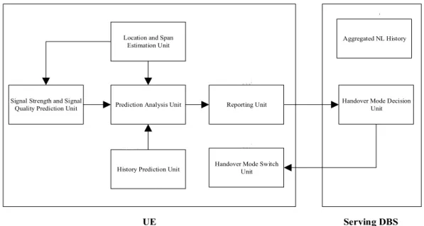
II. NETWORKARCHITECTURE ANDPROPOSEDSCHEME
We propose a memory-full context-aware HO scheme with mobility prediction and advance signalling to achieve a light-weight, signalling-efficient and fast HO procedure. We con-sider the dual connectivity RAN architecture with control/data plane separation [4] as it has been identified by the third generation partnership project (3GPP) as one of the candidate 5G RAN features [5]. Fig. 1 shows a high level overview of this architecture. It consists of a control base station (CBS) layer and a data base station (DBS) layer. The former is formed of macro BSs deployed at low frequency bands to provide ubiquitous connectivity, while the latter is formed of small
Active UE Active UE
Idle UE
Figure 1: Dual Connectivity RAN with control/data plane separation
BSs deployed at high (or low) frequency bands to provide on-demand high data rate transmission. The control/data separa-tion architecture (CDSA) requires the active UE to maintain a dual connection with both the CBS and the DBS, while idle UE (and detached UE accessing the network) maintain a single connection with the CBS only [4], [6], [7]. The DBS is invisible to both detached and idle UE, and its on-demand connection with the active UE is established and assisted by the CBS.
The dual connection feature of the CDSA coupled with con-textual information enable implementing fast and predictive HO schemes at the DBS layer. Predicting the UE mobility (at DBS level rather than the exact location) allows the source and the candidate DBSs to prepare and reserve resources in advance, which in turn could simplify the HO process and minimise the associated monitoring overhead, RAN signalling and interruption time [8], [9]. In the conventional RAN architecture, the predictive strategies have tight constraints since an incorrect prediction with a break-before-make HO can lead to detaching the UE from the network. In other words, an incorrect prediction in the conventional RAN does not only increase the HO latency and signalling overhead, but also it requires a new UE-network connection establishment. On the other hand, the CDSA offers relaxed constraints in implementing predictive HO management strategies. An incorrect DBS prediction in the CDSA does not require UE-network connection re-establishment, since the UE maintains another low rate connection with the CBS. In this direction, we propose predictive mobility management at DBS-level under CDSA configuration.
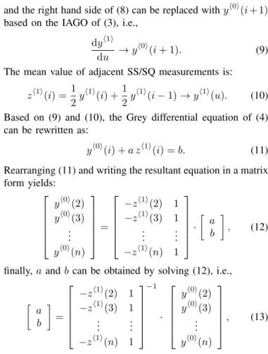
The proposed scheme depends on DBS SS and/or SQ prediction performed by the UE. This prediction is aided by UE context information such as location, direction and speed, in addition to statistical historical information based on either the UE HO history or the aggregated per-DBS Neighbour List (NL) HO history. A short-term memory for the RF measurements and a long-term memory for the HO history are considered, hence we describe this scheme as a memory-full context-aware mobility management approach. The predicted DBS is reported on an event basis to the serving (i.e., the source) DBS, which decides the reporting criteria and the HO mode to be followed by the UE. The
Signal Strength and Signal
Quality Prediction Unit Prediction Analysis Unit Location and Span
Estimation Unit
History Prediction Unit
Reporting Unit 102
101
103.a
104 105
Handover Mode Decision Unit
Handover Mode Switch Unit 107 106 UE Serving DBS Aggregated NL History 103.b
Figure 2: System model of the memory-full context-aware predictive handover scheme
prediction process is triggered only once when a certain prediction triggering threshold is reached. As shown in Fig. 2, the memory-full context-aware predictive DBS HO scheme comprises a location and span estimation unit, a SS and SQ prediction unit, a history prediction unit, a prediction analysis unit, a reporting unit, a HO mode decision unit and a HO mode switch unit.
The UE periodically measures SS and SQ of the serving
DBS and the top-m other detectable DBSs at every
measure-ment gap as in current standards. The 3GPP Measuremeasure-ment Reporting and Control (MRC) [10] may be re-used as an example of this measurement and optional reporting mecha-nism. The reported strongest or best quality DBSs are limited
to m per DBS categorisation as the measurement interval
is limited and measurement power consumption and normal transmission need to be balanced against the accurate mea-surement report (MR) cycle. The SS and SQ prediction unit
stores measurements of a subset of the top-mdetectable DBSs
that reside within the angular span of the UE direction/speed. The location and span estimation unit triggers the prediction process when the UE reaches the inner edge of cell (EoC) boundary of the serving DBS. The latter can be defined based on a distance threshold or a SS/SQ threshold. When the prediction is triggered, the SS and SQ prediction unit uses the stored measurements to predict SS and/or SQ of the serving DBS and the candidate DBSs.
The prediction analysis unit evaluates the predicted SS/SQ to determine if a certain DBS HO criteria is satisfied. If the predicted SS and/or SQ of a neighbouring DBS meets the HO criteria, then the prediction analysis unit queries the history prediction unit. The latter provides the prediction analysis unit with the probability of successful HO based on either the UE HO history or the DBS aggregated HO history. Based on these metrics as well as the predicted HO time, the prediction analysis unit may command the reporting unit to generate a new light-weight report called predictive measurement report
(PrMR) and sends it to the serving DBS. This PrMR is sent only once as opposed to the periodic MR transmission in the conventional HO approach. At the serving DBS side, the HO mode decision unit evaluates the PrMR and commands the UE to operate either in a predictive mode or revert back to the conventional non-predictive mode. In the former, the conventional MR is suspended, the HO-related RAN signalling is performed in advance and HO control is delegated to the UE. On the other hand, the non-predictive mode follows the conventional HO procedure where the HO decision is taken by the serving DBS after the HO criteria is met. Fig 3 shows a signalling flow diagram for the HO process based on the LTE X2 HO approach. The operation, algorithms and interactions of the proposed units are formulated and described in the following sections.
III. MEMORY-FULLPREDICTIONUNITS
A. Signal Strength/Quality Prediction
Fig. 4 shows an exemplary operation of the SS and SQ prediction unit. It contains a short-term memory that stores
the most recent n active state measurements of the DBSs
that reside within the angular span of the UE direction/speed.
In other words, the SS/SQ prediction window size is n
measurements per DBS. The SS/SQ prediction is based on measurement trends. To minimise the UE storage requirements and remove signal fading/fluctuation effects, Grey system theory [11] is adopted as the trending approach. The Grey theory has been used in several fields, e.g., for disaster, season and sequence prediction. It requires limited amount of input data and implicitly averages this data. The basic concept depends on translating the data sequence into a monotonic increasing function, representing this function by a differential equation and solving it to find the model’s parameters. For the
problem under study (i.e., SS/SQ prediction), a GM(1,1)1Grey
1
the first 1 means the model uses first order differential equations, while the second 1 means there is one variable.
UE Source DBS target DBS Predicted target DBS Actual MME S-GW a. Advance HO preparation Admission control b. Advance HO ACK Process
c. Advance SN status transfer Process Measurement reports HO decision 1. HO cancelation request Process 2. HO cancelation ACK Process 3. HO preparation request Admission control 4. HO preparation ACK Process 5. SN status transfer Process 6. HO command Detach from source DBS and access target DBS 7. HO confirm Process
8. Path switch request
Process
9. Update U-plane request Process 10. Update U-plane response Process
11. Path switch ACK
Process
12. UE context release
Process HO
triggered . . . . . . . . .
Figure 3: Signalling flow diagram for predictive and non-predictive HO scenarios, based on the LTE X2 HO procedure. Signalling messages in non-predictive HO: 3, 4, 5, 6, 7, 8, 9, 10, 11, 12. Sig-nalling messages in predictive HO with correct prediction (Network decision): 6, 7, 8, 9, 10, 11, 12. Signalling messages in predictive HO with correct prediction (HO control delegated to UE): 7, 8, 9, 10, 11, 12. Signalling messages in predictive HO with incorrect prediction: 1, 2, 3, 4, 5, 6, 7, 8, 9, 10, 11, 12. Acronym ACK: Acknowledgement, SN: Sequence Number.
model [11] can be constructed for each DBS as:
• The original SS/SQ measurements stored in the
short-term memory are represented as a time series given by: yh0i(i) =yh0i(1), yh0i(2), ... , yh0i(n), (1)
where the superscripth0imeans original SS/SQ
measure-ments (i.e., before processing) andi = 1,2,3, ... , n is
the measurement index.
• An accumulated generating operation (AGO) translates
yh0i(i)to a monotonic increasing function yh1i(i)as:
yh1i(i) =AGOnyh0i(i)o = yh0i(1), 2 X i=1 yh0i(i), ... , n X i=1 yh0i(i) ! . (2) 𝑖 = 1 𝑖 = 2… … … 𝑖 = 𝑛 − 1 𝑖 = 𝑛 Measured Predicted SS/SQ Time
Measured Measured Measured Measured Short term memory: most recent 𝑛 measurements
… … … … … … … … … ∆𝑔 Predicted … … … … … … … … … Serving DBS Candidate DBS 𝑖 = 𝑛 + 1 𝑖 = 𝑛 + 𝐼𝑝
Figure 4: Exemplary operation of the signal strength and signal quality prediction unit
• Based on (2), an inverse accumulated generating
opera-tion (IAGO) can be formulated as:
yh1i(i) =yh1i(i−1) +yh0i(i). (3)
• The GM(1,1) model is defined by the following equation:
dyh1i
du +a y
h1i
=b, (4)
whereais the develop parameter andbis the grey input.
The solution to (4) at time index iis:
yh1i(i+ 1) = yh1i(1)− b a e−a i+b a = yh0i(1)− b a e−a i+b a. (5)
By substituting the IAGO of (3) in (5), the predicted SS/SQ
one measurement gap in advanceyph0i(i+ 1)can be expressed
as: yhp0i(i+ 1) = e −a i (1−ea) yh0i(1)−b a . (6)
Similarly, the predicted SS/SQjmeasurement gaps in advance
can be formulated as:
yhp0i(i+j) = e−a(i+j−1)(1−ea) yh0i(1)−b a . (7)
Equation (7) can be used to predicted a series of SS/SQ
measurements. However, the model parameters a andb need
to be calculated before the prediction is performed. These parameters can be obtained by expressing the derivative in (4) as:
dyh1i
du →y
h1i
and the right hand side of (8) can be replaced withyh0i(i+ 1)
based on the IAGO of (3), i.e.,
dyh1i
du →y
h0i
(i+ 1). (9) The mean value of adjacent SS/SQ measurements is:
zh1i(i) =1 2y h1i(i) +1 2y h1i(i −1)→yh1i(u). (10)
Based on (9) and (10), the Grey differential equation of (4) can be rewritten as:
yh0i(i) +a zh1i(i) =b. (11)
Rearranging (11) and writing the resultant equation in a matrix form yields: yh0i(2) yh0i(3) .. . yh0i(n) = −zh1i(2) 1 −zh1i(3) 1 .. . ... −zh1i(n) 1 · a b , (12)
finally,aandb can be obtained by solving (12), i.e.,
a b = −zh1i(2) 1 −zh1i(3) 1 .. . ... −zh1i(n) 1 −1 · yh0i(2) yh0i(3) .. . yh0i(n) , (13)
The SS and SQ prediction unit uses this model to predict SS
and SQ of the serving DBS and a subset of the top-m other
detectable DBSs. These results are fed to the prediction analy-sis unit. It is worth mentioning that other trending techniques, such as polynomial fitting or sample extrapolation, can be used instead of the Grey model.
The expected HO time can be predicted based on rate of SS/SQ degradation. The measurement prediction is a time-series prediction, and it is performed on a sample-basis. Thus
if the measurement gap ∆g is constant (such as in current
standards), the SS and SQ prediction unit predicts a series of measurements until the HO criteria is satisfied (see Fig. 4).
For example, if the prediction is performed forIp samples in
advance (i.e., assuming that the current measurement index is
n, and the predicted SS/SQ that satisfies the HO criteria has
indexn+Ip), then the predicted remaining time for HO is:
Predicted HO time=Ip·∆g. (14)
B. History Prediction
The history prediction unit provides statistical historical information based on a long-term memory that helps the prediction analysis unit to confirm or reject the measurement-based HO prediction. It calculates the HO probability from the serving DBS to the predicted DBS based on either the aggregated NL HO history [12], [13] or the UE HO history. The former is already available in current standards at the network side in the form of a HO frequency table, and it provides statistical information based on the crowd behaviour. Table I provides an illustrative example of the NL HO history
Table I: Aggregated handover history in the long-term memory
From To
DBSa DBSb ... DBSk DBSl
DBSa 0 Ca,b ... Ca,k Ca,l
DBSb Cb,a 0 ... Cb,k Cb,l
... ... ... ... ... ...
DBSk Ck,a Ck,b ... 0 Ck,l
DBSl Cl,a Cl,b ... Cl,k 0
in a table format, whereCi,j is the NL-based aggregated HO
count from DBSi to DBSj. Typically, each row in Table I is
maintained by the source DBS. This NL HO history can be translated into a transition probability. For instance, the
NL-based transition probability ti,j from DBSi to DBSj can be
obtained by: ti,j= X u,∀u∈Ni Ci,j Ci,u , (15)
where Ni is the neighbour list of DBSi, i.e., a set of all the
DBSs that are neighbours to DBSi.
The NL-based history can be used for DBSs covering areas characterised by high batch HO rates. For example, where multiple UE on a train perform simultaneous HOs. However, the NL-based approach may not be suitable for individual users since it provides a coarse and less accurate estimate based on the crowd behaviour. This suggests a UE-based approach where individual users maintain separate statistical information based on their own history. This can be achieved by maintaining HO history tables as in Table I for each user,
i.e., ti,j is computed for each user based on their own Ci,j
values, or alternatively ti,j can be computed by using our
online history-based prediction scheme in [9].
IV. CONTEXT-AWAREASSISTANCEUNITS
A. Location and Span Estimation
The main objective of this unit is minimising the UE pro-cessing load and storage requirements. The prediction process in Section III-A can be continuously executed until a target DBS is found. However, such a continuous operation may not be feasible from battery and processing perspectives. A more convenient design approach is to trigger the prediction process when a certain triggering criteria is satisfied. This suggests a two boundary DBS cell structure, where the prediction is triggered at the inner boundary while the actual HO is performed at the outer boundary. Fig. 5 shows two approaches that can be used by the location and span estimation unit to trigger the prediction process at the inner boundary, based on the UE location w.r.t. the serving DBS, i.e., centre of cell (CoC) or EoC. Notice that the CoC/EoC classification is based on the inner boundary.
These approaches include position-based distance calcu-lation and serving DBS signal measurements. The former requires the serving DBS to broadcast its location, e.g., in the form of longitude and latitude. Then, the distance between the UE and the serving DBS can be calculated based on the UE position (provided by either a GPS or other positioning
𝑑𝑠.𝑡ℎ𝑟 𝑦𝑠.𝑡ℎ𝑟 0 Serving DBS CoC EoC Inner boundary Outer boundary
Figure 5: UE location estimation and CoC/EoC prediction triggering threshold 0 20 40 60 80 100 0 0.1 0.2 0.3 0.4 0.5 0.6 0.7 0.8 0.9 1
Predicted measurement precision (%)
Cummulative distribution function
advance period = 1 measurement gap advance period = 5 measurement gaps advance period = 25 measurement gaps advance period = 50 measurement gaps advance period = 75 measurement gaps
Figure 6: Predicted measurement precision with several advance periods, 5 UE per DBS,V=10 km/hr
techniques). When this distance equals to or greater than a
certain threshold ds.thr and it is increasing, then the UE
location is EoC and the prediction process is triggered. The second approach, i.e., the serving DBS signal measurements, utilises the measured SS/SQ from the serving DBS to trigger the prediction process. When the serving DBS SS/SQ drops
below a certain thresholdys.thrh0i , then the UE location is EoC
and the prediction process is triggered.
An appropriate setting of ds.thr and/or y
h0i
s.thr is of great
importance in improving the performance of the proposed
scheme. A large ds.thr (i.e., low yhs.thr0i ) setting may result
in a too late prediction, i.e., the HO may happen before the prediction process is triggered. On the other hand, a
small ds.thr (i.e., high y
h0i
s.thr) setting may lead to a too
early prediction. This in turn increases the error probability, due to the large gap between the time when the prediction is performed and the time when the actual HO happens. In addition, radio channel and/or UE direction will have a higher changing probability when the actual HO happens. As an illustrative example, Fig. 6 shows simulation results for the measurement prediction precision with several prediction
advance periods. As can be noticed, the prediction of theith
SS/SQ measurement is more accurate than the prediction of
thejth SS/SQ measurement, wherei<j.
Assuming a constant speed V and a hysteresis-based HO
criteria, i.e., the HO happens if the following condition is true:
logyhn0i ≥logyhs0i + log (Θ), (16) where ysh0i and yh 0i
n are the SS/SQ of the serving and the
neighbouring DBSs, respectively,Θis the HO hysteresis, and
the parameters in (16) are in linear scale. A HO hysteresis needs to be applied to the trend to ensure that prevailing conditions only are acted on to avoid HO ping-pong. For
a general path loss model χRξ, where χ is the
distance-independent path loss component, Ris the distance between
the Tx and the Rx, andξis the path loss exponent. Then it can
be proved that the actual HO happens after Ip measurements
referenced to the prediction triggering point, where Ip is
expressed as: Ip= qsΘ qn 1ξψ−d s.thrcos(φs) cos(φn) −ds.thr V ∆g 1 +cos(φs) cos(φn) qsΘ qn 1ξ , (17)
whereqsandqnare the transmit power of the serving and the
neighbouring DBSs, respectively, ψ is the inter-site distance,
φsis the angle between the line connecting the DBSs and the
line connecting the serving DBS with the UE location when
the HO happens,φn is the angle between the line connecting
the DBSs and the line connecting the neighbouring DBS with the UE location when the HO happens. It can be noticed that (17) depends on the UE speed. Thus using a DBS-based unified triggering threshold for all users implies that different
users will have different Ip values. Expressed differently, if
the prediction is triggered at the same location for all users, then low speed users will have to predict more measurements than high speed users. This may increase the error probability and decrease the prediction precision as shown in Fig. 6. This suggests a UE-specific prediction triggering threshold
ds.thr.U E that takes into account network parameters as well
as UE parameters. This threshold can be obtained by solving
(17) fords.thr, i.e., ds.thr.U E= q sΘ qn 1ξψ−I pV∆g cos(φs) cos(φn) −IpV∆g 1 +cos(φs) cos(φn) qsΘ qn 1ξ . (18)
The UE angular span is utilised to narrow down the can-didate DBS set. A high speed user usually has a smaller span (i.e., probability of changing the direction is small) as compared with a low speed user. This allows the former to store and process measurements of a smaller number of DBSs as compared with the latter. The location and span estimation
unit calculates the UE angular spanΩby
Ω = 2πe−η V, (19)
where η is the span gradient. Different DBSs can define
different values for η which can be learned from the users’
behaviour. For instance, a highway DBS may define a large gradient which results into a small span (i.e., a low mobility in a highway may be attributed to traffic conditions rather
than to a direction change intention). A new span is defined when the UE changes its speed abruptly, when the UE changes its direction by an angle larger than the initial span, or at
regular time intervals. Based on the location of the top-m
detectable DBSs, the location and span estimation unit selects the DBSs that reside within the UE span as candidates for the prediction process and store their measurements in the short-term memory. This result is fed to the SS and SQ prediction unit.
B. Prediction Analysis and Handover Mode Decision
The prediction analysis unit evaluates the predicted SS/SQ to determine if a certain HO criteria is satisfied. The latter is left as an implementation aspect to ensure a generic prediction scheme that does not depend on a particular HO model. For instance, the condition of (16) can be used as an example for the HO criteria. The prediction analysis unit confirms/rejects the measurement-based prediction based on the UE HO history
and the predicted HO time. Consider ts,p as the transition
probability from the serving DBSs to the measurement-based
predicted DBSp, based on either the crowd behaviour or the
individual user behaviour as explained in Section III-B. Define
tminas the minimum HO probability to confirm the prediction
from a history perspective. Then the prediction analysis unit confirms the measurement-based prediction if the following condition is true:
ts,p≥tmin, (20)
and it commands the reporting unit to send a PrMR, which contains the predicted DBS along with the predicted remaining time for HO given by (14). Otherwise, the prediction analysis unit rejects the measurement prediction. Notice that the an-gular span is accounted for in the monitoring and processing
phase (i.e.,ts,p belongs to one of the DBSs that reside within
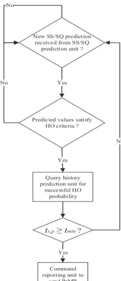
the UE angular span). Fig. 7 provides a flowchart for the operation flow of the prediction analysis unit.
The HO mode decision unit decides the type of HO to be followed by the UE, i.e., predictive or non-predictive HO. In the former, the conventional MRs are suspended, the HO decision and preparation are performed in advance, and HO control is delegated to the UE. It is worth mentioning that the HO mode decision unit can be located at the UE side and integrated with the prediction analysis unit, thus the outcome of the latter implicitly defines the HO type. If the final decision has to be taken based on additional policies defined by the network (i.e., network-controlled UE-assisted decision), then the HO mode decision unit can be moved to the DBS side as shown in Fig. 2.
V. PERFORMANCEEVALUATION
A. Prediction Threshold Analysis
Fig. 8 shows effect of the UE speed on the expected HO time (in measurement gaps) referenced to the prediction trig-gering point, with a unified trigtrig-gering threshold for all users.
The considered network parameters are: qs=qn=38 dBm,
ψ=130 m and ∆g=200 ms. A positive Ip value means
that the HO will happen after this value, while a negative
New SS/SQ prediction received from SS/SQ
prediction unit ?
Yes
Predicted values satisfy HO criteria ? Yes No No No Query history prediction unit for
successful HO probability ts,p ≥ tmin? Command reporting unit to send PrMR Yes
Figure 7: Flowchart of the operation flow and decisions of the prediction analysis unit
Ip value means a too late prediction (i.e., the HO already
happened before the prediction process is triggered). It can
be noticed in Fig. 8a that using a unified ds.thr value for
all users could result in a too early prediction especially
for low speed users. For instance, with ds.thr=20 m then
a low speed user with V=5 km/hr will start the prediction
process 188 measurement gaps in advance before the actual HO happens. As discussed in Section IV-A and depicted by Fig. 6, such an early prediction has a higher probability of error due to the fact that the prediction precision decreases as the advance period increases. On the other hand, using a large
ds.thr setting of 100 m results in a too late prediction, e.g.,
with V=5 km/hr then the prediction process starts after the
actual HO happens by 99 measurement gaps.
Fig. 8b indicates that the speed effect on the expected HO time (with a unified triggering threshold) is significantly influenced by the HO hysteresis. It can be seen that increasing
the hysteresisΘincreases the slope (in absolute value) of the
HO time vs speed graph whends.thr is constant for all users.
This indicates that a low hysteresis setting may be appropriate
when ds.thr is unified for all users. Nonetheless, the HO
hysteresis provides other benefits such as delaying the HO to avoid HO ping-pongs and it removes the SS/SQ fluctuation
effects. As a result, decreasingΘmay come at the expense of
0 5 10 15 20 25 30 35 40 45 50 55 60 65 70 75 80 −100 −50 0 50 100 150 200
User speed (km/hr)
I p (measurement gap)The UE needs to correctly predict the measurement reports up to j gaps away. Hysteris= 2 dB, measurement gap = 200 ms, ISD = 130 m, serving power = 38 dBm, neighbour power = 38 dBm
ds.thr= 20 m ds.thr= 40 m ds.thr= 60 m ds.thr= 80 m ds.thr= 100 m
(a) Effect ofds.thr, with hysteresis=2 dB
0 5 10 15 20 25 30 35 40 45 50 55 60 65 70 75 80 0 10 20 30 40 50 60 70 80 User speed (km/hr) I p (measurement gap)
The UE needs to correctly predict the measurement report up to j gaps away. dsthr= 60 m, measurement gap = 200 ms, ISD = 130 m, serving power = 38 dBm, neighbour power = 38 dBm Hysteresis= 0 dB
Hysteresis= 1 dB Hysteresis= 2 dB Hysteresis= 3 dB Hysteresis= 4 dB
(b) Effect of hysteresis, withds.thr=60 m
Figure 8: User speed vs expected handover time referenced to prediction triggering point with a unified triggering threshold for all users
The observations in Fig. 8 motivate a UE-specific prediction triggering threshold, which is provided in Fig. 9. It can
be noticed that ds.thr.U E is inversely proportional to the
UE speed. Expressed differently, low speed users start the prediction process at a larger distance from the serving DBS as compared with high speed users. This ensures that all users predict the same number of SS/SQ measurements, which in turn allows to set a maximum advance period in order to control the prediction precision and error probability. For example, to ensure that the prediction process does not start more than 8 measurement gaps before the actual HO happens,
then a user with V=5 km/hr and V=80 km/hr triggers the
prediction process at 70 m and 37 m, respectively, from the serving DBS as shown in 9a. Since the expected HO time is inversely proportional to the distance from the serving DBS,
then increasing the advance periodIp reducesds.thr.U E. On
the other hand, Fig. 9b indicates that the UE-specificds.thr.U E
and the HO hysteresis have a proportional relationship. This can be linked to the fact that the hysteresis delays the actual HO. Hence, for a fixed advance prediction period target,
0 5 10 15 20 25 30 35 40 45 50 55 60 65 70 75 80 0 10 20 30 40 50 60 70 80 User speed (km/hr)
UE−specific prediction triggering threshold (m)
Ip= 1 measurement gap
Ip= 2 measurement gaps
Ip= 4 measurement gaps
Ip= 8 measurement gaps
Ip= 16 measurement gaps
(a) Effect ofIp, with hysteresis=2 dB
0 5 10 15 20 25 30 35 40 45 50 55 60 65 70 75 80 45 50 55 60 65 70 75 80 User speed (km/hr)
UE−specific prediction triggering threshold (m)
Optimum prediction triggering threshold. j= 4 measurement gaps, measurement gap = 200 ms, ISD = 130 m, serving power = 38 dBm, neighbour power = 38 dBm
Hysteresis= 0 dB Hysteresis= 1 dB Hysteresis= 2 dB Hysteresis= 3 dB Hysteresis= 4 dB
(b) Effect of hysteresis, with Ip=4
Figure 9: User speed vs UE-specific prediction triggering threshold
a higher hysteresis setting increases the required prediction triggering distance from the serving DBS.
B. Prediction Statistics and Gains
System level simulations have been performed to assess performance and gains of the proposed DBS HO scheme. Table II provides the considered simulation parameters which are mostly aligned with the assumptions in [14]. Fig. 10 shows prediction accuracy and statistics for several SS trig-gering thresholds and HO hysteresis values. It can be noticed that this scheme provides a 90% prediction accuracy when
yhs.thr0i ≥ −62 dBm and HO hysteresis is used (i.e.,Θ>0 dB).
In addition, it significantly reduces the percentage of incorrect predictions that are not rejected by the prediction analysis
unit. Precisely, only 2.5%−9.6% of the predictions resulted
in HOs to DBSs other than the actual target DBSs. A very
low SS triggering threshold ofys.thrh0i =−64 dBm with a low
(or no) HO hysteresis setting results in a significant number of too late predictions. This can be traced to the fact that a low (or no) hysteresis results in an early HO while a low SS triggering threshold delays the prediction process. Expressed
Table II: Simulation parameters
Parameter Value
Network layout Hexagonal grid, 19 omnidirectional DBSs
Inter-site distance 130 m
DBS transmit power 38 dBm
Transmit mode SISO (Single Input Single Output)
User density 5 UE/DBS
User speed 10 km/hr for 100% of the users
Channel model 3GPP Typical Urban [15]
Path loss model 3GPP Urban [16]
Frequency 2 GHz
Bandwidth 10 MHz
Scheduler Round robin
Measurement gap 200 ms −64 −62 −60 −58 0 10 20 30 40 50 60 70 80 90 100
SS prediction triggering threshold y<0>s.thr (dBm)
Percentage (%)
Prediction statistics with hysteris= 2 dB
Correct timely predictions Incorrect predictions No candidate DBS is found Too late (missed) predictions
(a) Effect ofyhs.thr0i , with hysteresis=2 dB
0 2 4 6 0 10 20 30 40 50 60 70 80 90 100 Handover hysteresis (dB)
Percentage (%)
Prediction statistics with Sthr= −62 dB
Correct timely predictions Incorrect predictions No candidate DBS is found Too late (missed) predictions
(b) Effect of hysteresis, withyhs.thr0i =−62 dBm
Figure 10: Prediction statistics of the measurement-based context-aided predictive DBS handover scheme
differently, in environments/scenarios where HO hysteresis is not used, then the location and span estimation unit needs to be configured to start the prediction process early (i.e., high
ys.thrh0i or smallds.thr setting).
To evaluate HO latency of the proposed scheme, the approach of [17] has been followed by assuming that the transmission delay for different messages between the same
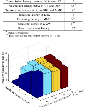
Table III: Latency values for handover signalling messages
Latency description Value (ms)
Transmission latency between DBSs over X2 5
Transmission latency between UE and DBS 6.5?
Transmission latency between DBS and MME 8.5
Processing latency at DBS 4
Processing latency at MME 5??
Processing latency at S-GW 5??
Detach and access latency 12
?
Includes processing.
??
Does not include UE context retrieval of 10 ms.
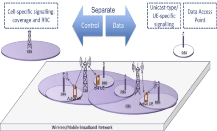
−64 −62 −60 −58 0 2 4 6 0 10 20 30 40
SS prediction triggering threshold
y<0>s.thr(dBm) Handover hysteresis (dB)
Predicitve handover gain (%)
Figure 11: Handover signalling latency reduction
source-destination pair is the same irrespective of the message size. Similarly, the processing delay for different messages at the same node is constant. In addition, it has been assumed that the mobility management entity (MME) and the serving gateway (S-GW) are located in the same location, thus the transmission delay between these nodes is negligible. Table III provides the latency values which are based on the feasibility study reported in [18] for the intra-LTE X2 HO procedure.
Fig. 11 shows gains of the proposed scheme in terms of signalling latency reduction w.r.t. the conventional HO proce-dure. Based on the latency parameters of Table III, it can be concluded that the memory-full context-aware predictive HO scheme reduces the DBS HO latency by 33.6% as compared with the conventional HO. Fig. 11 also indicates that the highest gains can be achieved either with a high hysteresis and a low SS/SQ (i.e., a large UE/serving-DBS distance) triggering threshold, or with a low hysteresis and a high SS/SQ (i.e., a small UE/serving-DBS distance) triggering threshold.
VI. CONCLUSION
Predictive HO signalling at DBS-level is proposed in this paper. With the main objective of minimising the CDSA HO-related RAN signalling and the associated latency and monitoring load, a memory-full context-aware predictive DBS HO is proposed. This scheme includes a proactive HO mode selection model to minimise the HO signalling latency, since the predictive HO management strategies may not be suitable
in some cases, e.g., unpredictable users with highly random mobility profiles or users visiting new DBSs. Considering the dual connectivity feature of the CDSA, such a predictive approach can be applied with relaxed constraints.
The proposed scheme is operated at the UE, and it predicts the expected HO time in addition to the target DBS. It com-bines physical proximity (i.e., location information at the UE) to a virtualised UE view of DBS coverage, RF performance derived from SS/SQ measurements, context information and HO history. The SS/SQ measurements are modelled as a time series in a Grey fashion to predict future HO events and the remaining time for HO. In addition, the UE speed and direction are utilised to minimise the storage and processing requirements by narrowing down the candidate DBS set based on the UE angular span. A UE-specific prediction triggering threshold is formulated to improve the measurement prediction precision whilst minimising the UE processing load. For a certain advance prediction period (and hence a certain preci-sion target), it has been found that the UE-specific triggering threshold is inversely proportional (in distance format) and directly proportional (in SS/SQ format) to the UE speed. The switching point between predictive and conventional HO procedures is defined based on the successful HO probability which is obtained from the history prediction model.
Simulation results show that the proposed predictive scheme reduces the HO signalling latency by 33.6% as compared with the conventional LTE X2 HO procedure. These gains depend on network-defined HO parameters such as the HO hysteresis and transmit power, in addition to the UE-specific prediction parameters such as the prediction triggering threshold. This suggests an appropriate setting of both the network-defined and the UE-specific parameters to achieve the maximum gain.
ACKNOWLEDGEMENT
We would like to acknowledge the support of the University of Surrey 5GIC (http://www.surrey.ac.uk/5gic) members for this work.
REFERENCES
[1] J. G. Andrews et al., “What will 5G be,” IEEE Journal on Selected
Areas in Communications, vol. 32, no. 6, pp. 1065–1082, June 2014.
[2] Nokia Siemens Networks, “2020: Beyond 4G, radio
evolution for the gigabit experience,” White Paper,
August 2011. [Online]. Available: http://nsn.com/file/15036/
2020-beyond-4g-radio-evolution-for-the-gigabit-experience
[3] 3GPP, “Evolved Universal Terrestrial Radio Access (E-UTRA); Mobility enhancements in heterogeneous networks,” Technical Report, December 2012, 3GPP TR 36.839 version 11.1.0 Release 11. [Online]. Available: http://www.3gpp.org/DynaReport/36839.htm
[4] A. Mohamed, O. Onireti, M. Imran, A. Imran, and R. Tafazolli, “Control-data separation architecture for cellular radio access networks:
A survey and outlook,” IEEE Communications Surveys and Tutorials,
vol. 18, no. 1, pp. 446–465, Firstquarter 2016.
[5] 3GPP, “Study on scenarios and requirements for next generation access technologies,” Technical Report, June 2016, 3GPP TR 38.913 version 0.4.0 Release 14. [Online]. Available: http://www.3gpp.org/ DynaReport/38913.htm
[6] H. Ishii, Y. Kishiyama, and H. Takahashi, “A novel architecture for
LTE-B :C-plane/U-plane split and phantom cell concept,” inProc. of IEEE
Globecom Workshops, December 2012, pp. 624–630.
[7] X. Xu, G. He, S. Zhang, Y. Chen, and S. Xu, “On functionality
separation for green mobile networks: Concept study over LTE,”IEEE
Communications Magazine, vol. 51, no. 5, pp. 82–90, May 2013.
[8] A. Mohamed, O. Onireti, M. A. Imran, A. Imran, and R. Tafazolli, “Predictive and core-network efficient RRC signalling for active state
handover in RANs with control/data separation,”IEEE Transactions on
Wireless Communications, vol. 16, no. 3, pp. 1423–1436, March 2017. [9] A. Mohamed, O. Onireti, S. Hoseinitabatabae, M. Imran, A. Imran, and R. Tafazolli, “Mobility prediction for handover management in cellular
networks with control/data separation,” inProc. of IEEE International
Conference on Communications (ICC), June 2015, pp. 3939–3944.
[10] 3GPP, “Evolved universal terrestrial radio access (E-UTRA);
Radio resource control (RRC) protocol specification,” Technical Specification, April 2016, 3GPP TS 36.331 version 13.1.0 Release 13. [Online]. Available: http://www.etsi.org/deliver/etsi ts/136300 136399/ 136331/13.01.00 60/ts 136331v130100p.pdf
[11] D. Julong, “Introduction to grey system theory,” The Journal of grey
system, vol. 1, no. 1, pp. 1–24, 1989.
[12] H. Hu, J. Zhang, X. Zheng, Y. Yang, and P. Wu, “Self-configuration and
self-optimization for LTE networks,”IEEE Communications Magazine,
vol. 48, no. 2, pp. 94–100, February 2010.
[13] M. Amirijoo, P. Frenger, F. Gunnarsson, H. Kallin, J. Moe, and K. Zetterberg, “Neighbor cell relation list and physical cell identity
self-organization in LTE,” in Proc. of EEE International Conference
on Communications (ICC), May 2008, pp. 37–41.
[14] 3GPP, “Physical layer aspects for evolved Universal Terrestrial
Radio Access (UTRA) ,” Technical Report, September 2006,
3GPP TR 25.814 version 7.1.0 Release 7. [Online]. Available: http://www.qtc.jp/3GPP/Specs/25814-710.pdf
[15] ——, “Technical Specification Group Radio Access Network;
Deployment aspects,” Technical Report, January 2016, 3GPP
TR 25.943 version 13.0.0 Release 13. [Online]. Available:
http://www.3gpp.org/DynaReport/25943.htm
[16] ——, “Evolved Universal Terrestrial Radio Access (E-UTRA); Radio Frequency (RF) system scenarios,” Technical Report, January 2016, 3GPP TR 36.942 version 13.0.0 Release 13. [Online]. Available: http://www.3gpp.org/dynareport/36942.htm
[17] L. Wang, Y. Zhang, and Z. Wei, “Mobility management schemes at radio
network layer for LTE femtocells,” inProc. of IEEE 69th Vehicular
Technology Conference (VTC), April 2009.
[18] 3GPP, “Feasibility study for evolved Universal Terrestrial Radio Access (UTRA) and Universal Terrestrial Radio Access Network (UTRAN),” Technical Report, October 2012, 3GPP TR 25.912 version 11.0.0 Release 11. [Online]. Available: http://www.3gpp.org/DynaReport/ 25912.htm
Abdelrahim Mohamed (S’15–M’16) received the
B.Sc. degree (First Class) in electrical and elec-tronics engineering from the University of Khar-toum, Sudan, in 2011, the M.Sc. degree (distinction) in mobile and satellite communications, and the Ph.D. degree in electronics engineering from the University of Surrey, U.K., in 2013 and 2016. He is currently a Postdoctoral Research Fellow with ICS/5GIC, the University of Surrey, Surrey, U.K. He is currently involved in the RRM, MAC and RAN Management work area, and the New Physical Layer work area in the 5GIC at the University of Surrey. He is involved in the energy proportional eNodeB for LTE-Advanced and Beyond Project, the planning tool for 5G network in mm-wave band project, in parallel to working on the development of the 5G system level simulator. His research contributed to the QSON project, and the FP7 CoRaSat Project. His main areas of research interest include radio access network design, system-level analysis, mobility management, energy efficiency and cognitive radio. He secured first place and top ranked in the Electrical and Electronic Engineering Department, University of Surrey, during his M.Sc. studies. He was a recipient of the Sentinels of Science 2016 Award.
Muhammad Ali Imran (M’03, SM’12) received his M.Sc. (Distinction) and Ph.D. degrees from Imperial College London, UK, in 2002 and 2007, respectively. He is a Professor in Communication Systems in University of Glasgow, Vice Dean of Glasgow College UESTC and Program Director of Electrical and Electronics with Communications. He is an adjunct Associate Professor at the University of Oklahoma, USA and a visiting Professor at 5G Innovation centre, University of Surrey, UK, where he has worked previously from June 2007 to Aug 2016. He has led a number of multimillion-funded international research projects encompassing the areas of energy efficiency, fundamental perfor-mance limits, sensor networks and self-organising cellular networks. He also led the new physical layer work area for 5G innovation centre at Surrey. He has a global collaborative research network spanning both academia and key industrial players in the field of wireless communications. He has supervised 21 successful PhD graduates and published over 200 peer-reviewed research papers including more than 20 IEEE Transaction papers. He secured first rank in his B.Sc. and a distinction in his M.Sc. degree along with an award of excellence in recognition of his academic achievements conferred by the President of Pakistan. He has been awarded IEEE Comsoc’s Fred Ellersick award 2014, Sentinel of Science Award 2016, FEPS Learning and Teaching award 2014 and twice nominated for Tony Jean’s Inspirational Teaching award. He is a shortlisted finalist for The Wharton-QS Stars Awards 2014, Reimagine Education Award for innovative teaching and VC’s learning and teaching award in University of Surrey. He is a senior member of IEEE and a Senior Fellow of Higher Education Academy (SFHEA), UK. He has given an invited TEDx talk (2015) and more than 10 plenary talks, several tutorials and seminars in international conferences and other institutions. He has taught on international short courses in USA and China. He is the co-founder of IEEE Workshop BackNets 2015 and chaired several tracks/workshops of international conferences. He is an associate Editor for IEEE Communications Letters, IEEE Open Access and IET Communications Journal.
Pei Xiao (SM’11) is a professor at the Institute
for Communication Systems, home of 5G Inno-vation Centre (5GIC) at the University of Sur-rey. He is the technical manager of 5GIC, leading the research team at on the new physical layer work area, and coordinating/supervising research activities across all the work areas within 5GIC (www.surrey.ac.uk/5gic/research). Prior to this, he worked at Newcastle University and Queen’s Uni-versity Belfast. He also held positions at Nokia Networks in Finland. He has published extensively in the fields of communication theory and signal processing for wireless communications.
Rahim Tafazolli (SM’09) is a professor and the
Director of the Institute for Communication Sys-tems (ICS) and 5G Innovation Centre (5GIC), the University of Surrey in the UK. He has published more than 500 research papers in refereed journals, international conferences and as invited speaker. He is the editor of two books on “Technologies for Wireless Future” published by Wiley’s Vol.1 in 2004 and Vol.2 2006. He was appointed as Fellow of WWRF (Wireless World Research Forum) in April 2011, in recognition of his personal contribution to the wireless world. As well as heading one of Europe’s leading research groups.


![Table II provides the considered simulation parameters which are mostly aligned with the assumptions in [14]](https://thumb-us.123doks.com/thumbv2/123dok_us/10177901.2920142/9.892.79.418.87.620/table-ii-provides-considered-simulation-parameters-aligned-assumptions.webp)