DOTTORATO DI RICERCA IN
Automatica e Ricerca Operativa
Ciclo XXVIII
Settore concorsuale di afferenza: 01/A6 - RICERCA OPERATIVA Settore scientifico disciplinare: MAT/09 - RICERCA OPERATIVA
Mathematical Optimization for Routing
and Logistic Problems
Presentata da: Claudio Gambella
Coordinatore Dottorato
Relatore
Prof. Daniele Vigo
Prof. Daniele Vigo
Co-relatore
Prof. Andrea Lodi
List of Figures vii
List of Tables ix
1 Introduction 1
1.1 Conic Programming . . . 3
1.1.1 Conic Programs . . . 3
1.1.2 Second-Order Conic Programming . . . 5
1.1.3 Mixed-Integer Second-Order Conic Programming . . . 6
1.1.4 Solvers for (MI)SOCPs . . . 7
1.2 Stochastic Programming . . . 8
1.2.1 Two-Stage Stochastic Programming . . . 10
1.2.2 Multistage Stochastic Programming . . . 12
1.2.3 Measures and Bounds for Two-Stage Stochastic Programming. . 14
1.2.4 Measures and Bounds for Multistage Stochastic Programming. . 16
1.3 Lagrangian Relaxation and Lagrangian Decomposition . . . 17
1.3.1 Lagrangian Relaxation and Lagrangian Dual Problem . . . 17
1.3.2 Iterative Methods for Solving the Lagrangian Dual Problem . . . 18
1.3.3 Considerations on the Lagrangian Dual Problem Solution . . . . 20
1.3.4 Lagrangian Decomposition . . . 20
1.4 Invoking Optimization Solvers. . . 22
1.5 Thesis Overview . . . 23
2 Exact Solutions for the Carrier-Vehicle Traveling Salesman Problem 25 2.1 Introduction. . . 25
2.2 A MISOCP Model for Solving CVTSP . . . 27
2.3 A Benders-like Enumeration Procedure for Solving CVTSP . . . 29
2.3.1 Combinatorial Lower Bound for the CVTSP. . . 31
2.3.2 Ranking of TSP Solutions . . . 32
2.3.2.1 Detecting the Infeasibility of a Symmetric TSP Sub-problem . . . 33
2.4 Computational Results . . . 35
2.4.1 Results of the Benders-like Enumeration Algorithm. . . 35
2.4.2 Comparison Between BEA Version V2 and Optimization Solvers 39 2.5 Conclusions . . . 41
3 The Interceptor Vehicle Routing Problem: Formulation and
3.3 IVRP Formulation: General Case . . . 46
3.4 IVRP Formulation: Targets Moving Along a Fixed Line . . . 49
3.4.1 Valid Inequalities . . . 50
3.5 Lagrangian Decomposition. . . 52
3.5.1 Tightening the Lagrangian Bound . . . 55
3.5.2 Branching Strategy. . . 56
3.6 Implementation Details and Preliminary Computational Results . . . . 56
3.7 Conclusions . . . 63
4 Waste Flow Optimization: An Application in the Italian Context 65 4.1 Introduction. . . 65
4.2 Waste Management in Italy . . . 66
4.2.1 Municipal Waste Management . . . 68
4.2.1.1 Municipal Waste Production . . . 68
4.2.1.2 Municipal Sorted Waste Collection. . . 68
4.2.1.3 Municipal Waste Treatment and Disposal . . . 69
4.2.2 Industrial Waste Management. . . 70
4.2.2.1 Industrial Waste Production . . . 70
4.2.2.2 Industrial Waste Collection . . . 71
4.2.2.3 Industrial Waste Treatment and Disposal . . . 71
4.3 Waste Flow Optimization . . . 73
4.4 Model Formulation for Waste Allocation Problems . . . 75
4.4.1 Objective Function . . . 79 4.4.2 Flow Balance . . . 80 4.4.3 Flow Limitation . . . 80 4.4.4 Facility Deactivation . . . 80 4.4.5 Economies of Scale . . . 80 4.4.6 Additional Features . . . 81 4.4.6.1 Digester Facilities . . . 82 4.4.6.2 Temporary Storage . . . 83
4.4.6.3 Logic Constraints on Incoming Waste Flow . . . 84
4.5 Case Study . . . 84
4.5.1 The Decision Support System Solution . . . 85
4.5.2 Solution Approach . . . 86
4.5.2.1 Time Horizon and Time Granularity . . . 86
4.5.2.2 Waste Commodities and Network Topology Definition . 87 Waste types aggregation . . . 87
Waste sources aggregation . . . 87
Plants . . . 88
Distance Matrix. . . 89
4.5.2.3 Costs and Revenues . . . 89
4.5.2.4 Operations Modeling and Constraints . . . 90
4.6 Results. . . 90
4.6.1 Comparative Results for the Case Study . . . 91
4.6.2.1 Economic Key Performance Indicators with Landfill
Disposal Limitations. . . 95
4.6.2.2 Waste Flow Allocation to Facilities with Landfill Dis-posal Limitations . . . 96
4.7 Conclusions and Future Works . . . 96
5 A Solid Waste Management Problem with Stochastic Parameters at a Tactical Planning Level 99 5.1 Introduction. . . 99
5.2 Literature Review . . . 100
5.2.1 Strategic Planning . . . 100
5.2.2 Tactical Planning. . . 101
5.3 The Planning Problem . . . 102
5.4 Stochastic Models . . . 103
5.4.1 Two-Stage Multiperiod Formulation without Operational Actions105 5.4.2 Two-Stage Multiperiod Formulation with Operational Actions . 107 5.5 Scenario Generation . . . 110
5.6 Preliminary Computational Results. . . 111
5.6.1 Model (M1) . . . 112
5.6.2 Model (M2) . . . 112
5.7 Conclusions and Future Works . . . 113
6 Overview of Optimization Problems in Electric Car-Sharing System Design and Management 115 6.1 Introduction. . . 115
6.2 Strategic and Tactical Problems. . . 117
6.2.1 Location of Stations . . . 118
6.2.1.1 Location of Charging Stations for Ecar-sharing systems 119 6.2.1.2 Location of Charging Stations for Privately Owned Cars120 6.2.1.3 Location of Stations for Electric Taxi Cabs . . . 121
6.2.1.4 Location of Stations for Non-Electric Car-Sharing Sys-tems. . . 122
6.2.1.5 Summary, Open Problems and Possible Research Di-rections . . . 123
6.2.2 Allocation of Vehicles to Existing Stations . . . 124
6.2.2.1 Summary, Open Problems and Possible Research Di-rections . . . 124
6.3 Operational Problems . . . 124
6.3.1 Relocation of Vehicles for Multiple-Stations Car-Sharing . . . 125
6.3.1.1 User-Based Strategies . . . 125
6.3.1.2 Operator-Based Strategies . . . 126
6.3.1.3 Summary, Open Problems and Possible Research Di-rections . . . 129
6.3.2 Battery Swap . . . 131
6.3.2.1 Summary, Open Problems and Possible Research Di-rections . . . 133
rections . . . 135
6.3.4 Electric Vehicle Routing Problem . . . 136
6.3.4.1 Summary, Open Problems and Possible Research Di-rections . . . 139
6.4 Conclusions . . . 140
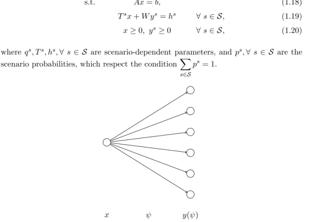
1.1 Two-stage scenario tree with|S|= 6 . . . 11
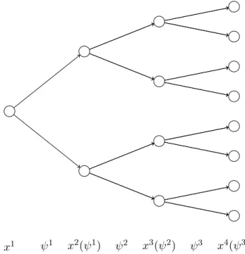
1.2 Multistage scenario tree with 4 stages and 2 branches per stage,|S|= 8 13
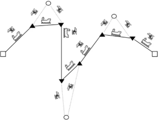
2.1 Schematic representation of a Carrier-Vehicle route. Squares represent the start and end location, circles are the target points, triangles are take-off and landing positions. Solid lines are the carrier paths and dotted lines are the vehicle ones. . . 26
3.1 A ride-sharing system with two vehicles and three customers . . . 44
4.1 A diagram representing the typical waste facilities network. SMW stands for Sorted Municipal Waste, ND is Non-Dangerous, PBT is Phisiochemi-cal BiologiPhisiochemi-cal Treatment, WtE is Waste to Energy, T&EE is Termal and Electrical Energy, Env. Eng. is Environmental Engineering, Pre.Tr. is Preliminary Treatments (see [135], in Italian). . . 67
4.2 Regional production of municipal waste per capita and regional percent-age ratio of sorted municipal waste collection (source ISPRA [147]) . . . 69
4.3 Percentage subdivision of IW total production in 2010. . . 71
4.5 An example of concave piecewise linear cost function of the waste flow . 81
4.6 OptiWasteFlow DSS: the Solution process (a) and an example of Graph-ical User Interface (b). . . 86
4.7 Location of facilities (left) and sources (right) in the Herambiente case study . . . 89
4.8 Changes on flow allocation as a consequence of introduced limitation of waste acceptance on a WtE facility . . . 91
5.1 The SWM network . . . 104
5.2 Two-stage multiperiod scenario tree related to formulation (5.1)-(5.11) with|S|= 3 andT = 12 . . . 107
5.3 Scenario tree associated with formulation (5.12)-(5.23) with|S|= 3 and
T = 12 . . . 110
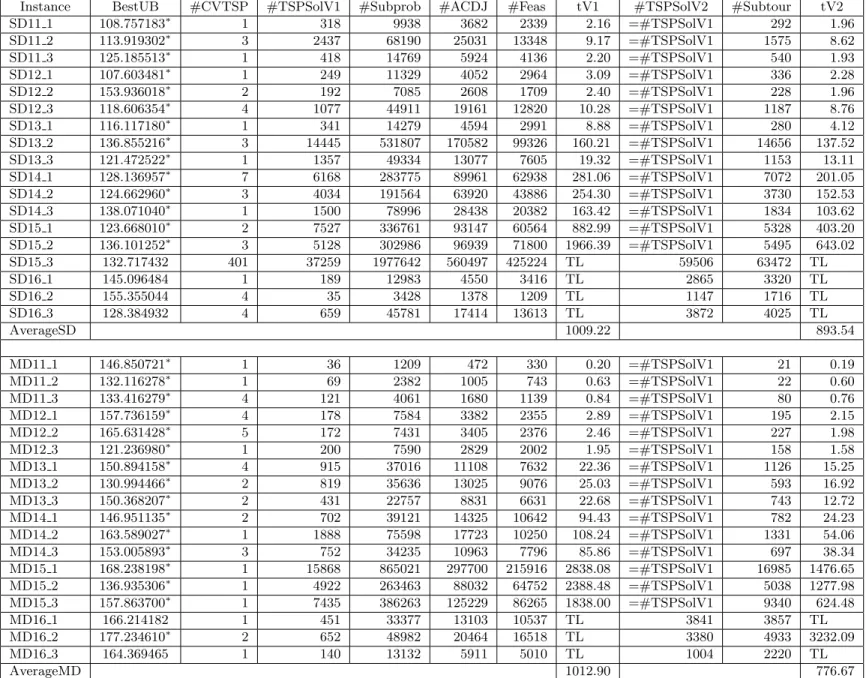
2.1 BEA - Instances SD and MD - Infeasibility detection versions V1, V2 . 37
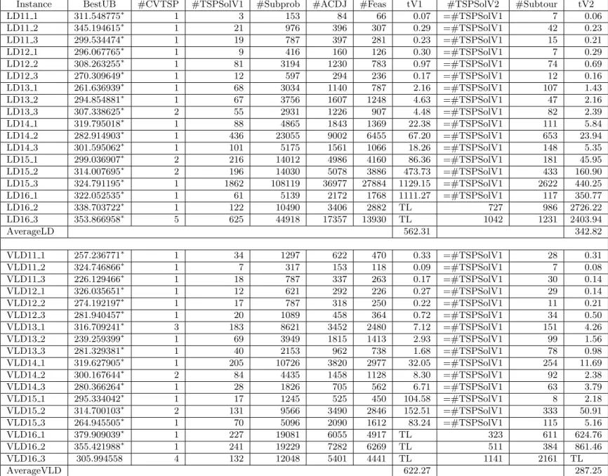
2.2 BEA - Instances LD and VLD - Infeasibility detection versions V1, V2 . 38
2.3 GAMS solver link versions . . . 39
2.4 Solvers comparison for the groups SD, MD, LD, VLD . . . 40
2.5 Time limit instances for each algorithm . . . 41
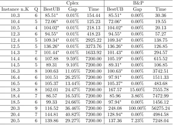
3.1 Cplex and Branch & Price comparison . . . 59
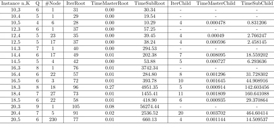
3.2 Branch & Price statistics . . . 60
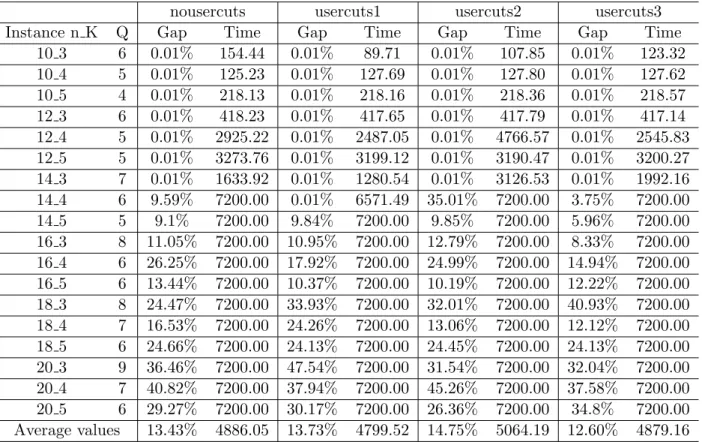
3.3 Valid inequalities . . . 61
3.4 Symmetry breaking constraints . . . 62
4.1 Breakdown of Herambiente plants network . . . 88
4.2 Comparison of main logistic and economic KPI: negative values means a reduction in the optimized solution with respect to the as-is solution.. 92
4.3 Percentage variation of total disposal cost in detail for various facilities and final destinations. . . 93
4.4 Percentage variation of treatment revenues in detail for some aggregated waste types and destinations. . . 93
4.5 Percentage variation in flow allocation among facilities and final desti-nations. . . 95
4.6 Percentage variation of total disposal cost in detail for various facilities and final destinations. Scenario with landfill disposal limitations. . . 96
4.7 Percentage variation of total disposal cost in detail for various facilities and final destinations. Scenario with landfill disposal limitations. . . 96
4.8 Percentage variation of treatment revenues in detail for some aggregated waste types and destinations. Scenario with landfill disposal limitations. 97 4.9 Percentage variation in flow allocation among facilities and final desti-nations. Scenario with landfill disposal limitations. . . 97
6.1 Classification of the literature related with location of charging stations. 119 6.2 Classification of the literature related with vehicles relocation (UB: user-based relocation strategy, OB: operator-based relocation strategy).. . . 125
6.3 Classification of the literature related with EV routing problems (SP: shortest path problem, VRP: vehicle routing problem). . . 139
• Mathematical Optimization
• Second-Order Conic Programming
• Mixed-Integer Second-Order Conic Programming
• Path Planning
• Mission Planning
• Traveling Salesman Problem
• Vehicle Routing Problem
• Branch-and-Price
• Lagrangian Relaxation
• Lagrangian Decomposition
• Waste Management
• Stochastic Programming
• Two-Stage Multiperiod Stochastic Programming
I am grateful to my supervisors Prof. Daniele Vigo and Prof. Andrea Lodi for their guidance and help in my research projects. I want to thank them also for the great mobility opportunities offered, which gave me personal enrichment and stimulated my Ph.D. activity.
Many thanks go to Dr. Bissan Ghaddar and Prof. Joe Naoum-Sawaya for supervising me during the internship in IBM Ireland. Their availability and listening skill have deeply stimulated me and made me feel part of a productive team.
Regarding the research on waste management of Chapter 5, I am thankful to Prof. Francesca Maggioni for her assistance, to the waste operator Herambiente SpA and the consulting company Optit Srl for sharing their real data.
I would like to thank the components of the group of Operations Research of the DEI, Dipartimento di Ingegneria dell’Energia elettrica e dell’Informazione of the University of Bologna, namely Prof. Paolo Toth, Prof. Enrico Malaguti, Prof. Michele Monaci, Dr. Valentina Cacchiani, Dr. Paolo Tubertini, Ph.D. students Maxence Delorme, Alberto Santini, Dimitri Thomopulos and the former member Dr. Tiziano Parriani. A particular mention goes to the Ph.D. student Sven Wiese, for his patience and presence during these years.
I would like also to thank the Ministero dell’Istruzione, dell’Universit`a e della Ricerca (MIUR) for the financial support given to my Ph.D. course.
Introduction
Mathematical optimization (also referred to asmathematical programming) is a branch
of applied mathematics that requires to solve a minimization or maximization problem subject to a set of constraints. The general form of representation of a constrained optimization problem is
minf(x) (1.1)
s.t. x∈X⊆Rn, (1.2)
where f is a real-valued function, calledobjective function, and thefeasible region X
is the subset of values of the decision variables x that satisfy the problem constraints, given in the form of equalities or inequalities. Note that every maximization problem can be equivalently converted in a minimization one.
Optimization problems can be viewed as mathematical formulations of decision prob-lems. The applications of mathematical modeling invest several areas, such as econ-omy, finance, engineering, scheduling, military, routing and logistic problems. The purpose of the optimization is to give a decision support system with quantitative tools, in contrast with qualitative criteria motivated by empirical experience and per-sonal judgement.
Two main classes of solution approaches for problems of form (1.1)-(1.2) are exact
methods and heuristic algorithms. The aim of an exact method is to select anoptimal
solution, namely a vector x of decision variables that belongs to set X and minimizes
the objective function f (i.e., f(x) ≤ f(x0) ∀ x0 ∈ X). When modeling a practical problem, the size of the optimization problem can be very large in terms of decision variables and constraints; in addition, a complete and accurate description of the set of the model entities may be an intractable task. In such situations, heuristics are adopted for finding solutions of good proven quality in a reasonable amount of time. A minimal classification of optimization problems produces four relevant categories:
• Linear Programming (LP) (Dantzig [75]): problems with objective function and constraints expressed by linear functions;
• Mixed-Integer Linear Programming (MILP) (see, e.g., Smith and Taskın [230]):
LPs in which (some) decision variables are required to assume integer values;
• Non-Linear Programming (NLP) (see, e.g., Bertsekas [36]): problems where
ob-jective function and constraints are represented by nonlinear functions;
• Mixed-Integer Non-Linear Programming (MINLP) (see, e.g., Belotti et al. [31]):
NLPs in which (some) decision variables are subject to integrality requirements.
Amongst nonlinear problems, an important distinction is made between Convex Pro-gramming (see, e.g., Boyd and Vandenberghe [45]) and Non-Convex Programming (see, e.g., Burer and Letchford [50]). Non-convex problems have a non-convex feasible region or a non-convex continuous relaxation, if integrality constraints are present. A primary implication of the non-convexity is that the optimization problem may have multiple optimal solutions. In Non-Convex Programming, the optimizer is mainly interested in finding locally optimal solutions, because proving the global optimality of a candidate solution may be a very difficult challenge.
The problem type affects the choice of the applicable methods for finding optimal so-lutions of the mathematical model. For practically solving large-scale problems, an initial approach is to invoke optimization solvers. Such commercial or non-commercial software contain solution algorithms that proved to be efficient and effective for spe-cific classes of optimization problems. The development of tailored algorithms on the specific optimization problem may be instead required for various reasons, such as low-ering the computational time required and dealing with the scalability of the model. In order to obtain information about the optimization problem, relaxed problems may be considered. Relaxations are modeling strategies that permit to consider substan-tially easier problems than the original one. A relaxation of (1.1)-(1.2) is an optimiza-tion problem
minfR(x) (1.3)
s.t. x∈XR⊆Rn (1.4)
that satisfies the conditions:
1. XR⊇X;
2. fR(x)≤f(x)∀ x∈X.
The two conditions ensure that solving a relaxation of a minimization problem provides
a lower bound on the optimal solution value. In the case of continuous relaxation of
used, for instance, in branch-and-bound methods (Land and Doig [166], Nemhauser and Wolsey [198], Papadimitriou and Steiglitz [203]).
This chapter is meant for laying the main theoretical basis of the research projects developed in the thesis. To this end, Sections 1.1 and 1.2 introduce two relevant classes of programming paradigms, Section 1.3 describe a solution method developed on the basis of a problem relaxation, and Section 1.4 summarizes the forms in which the optimization solvers have been used in the projects of the thesis. The practical relevance of the modeling paradigms and solution techniques introduced in this chapter will become more apparent over Chapters2,3and5. Finally, an overview of the thesis is given in Section 1.5.
1.1
Conic Programming
Conic Programming is a relevant subcategory of Convex Programming. The accurate representation of an optimization model is a central issue in Non-Linear Programming. While general non-linear constraints can be particularly tricky to handle, recognizing the conic property of a function allows to adopt tailored solution algorithms in order to efficiently find optimal solutions.
1.1.1 Conic Programs
Let K ⊂Rn be a cone (i.e., closed under multiplication by positive scalars). The set
K is said to beregular if it is convex, closed, it has a nonempty interior and it contains 0.
Let M be a m×nmatrix, µbe a vector of Rm and γ be a vector of Rn.
A conic program on K is an optimization problem of the form:
min
x∈Rn
{γTx:M x−µ∈K}. (1.5) Conic programs are polynomially solvable when the associated cones are “computa-tionally tractable” (i.e., admitting polynomial time membership/separation oracles) and the feasible region is appropriately bounded (Nemirovski [199]). In the case of problems on a cone from a family K of regular cones, fast interior point methods can be adopted: this motivates the interest in determining if a generic convex problem is representable as a conic problem, namely in aK-representable form.
of minimizing a linear objective function. Important and broad subclasses are given by the symmetric cones:
• K =Rm+, then problem (1.5) reduces to a Linear Programming problem (Dantzig [75]) min x∈Rn {γTx:M x−µ≥0}. (1.6) • K = p Y i=1 Lmi, where each Lmi ={(y, t) ∈ Rmi, y ∈Rmi−1, t∈ R:kyk2 ≤t} is a Lorentz cone. In this case, (1.5) is expressed in the form
min
x∈Rn
γTx (1.7)
kAix−bik2 ≥cTi x−di i= 1, . . . , p, (1.8)
where Ai is a mi ×n matrix, bi ∈ Rmi, ci ∈ Rn and di ∈ R. Problem (1.7
)-(1.8) is named as Conic Quadratic Programming (CQP) or Second-Order Conic Programming (SOCP) problem. Constraints (1.8) are called Conic Quadratic Inequalities (CQIs) or second-order cone constraints of dimension mi.
• K =
q
Y
i=1
Smi, where eachSmibelongs to the cone of positive semidefinite (i.e.,<0)
and symmetric mi ×mi matrices with the Frobenius inner product hA, Bi =
T r(AB).
Problem (1.5) therefore describes a Semi-Definite Programming (SDP) problem
min
x∈Rn{γ
Tx:A
ix−Bi≡x1Ai1+· · ·+xnAin−Bi <0 i= 1, . . . , q}, (1.9)
where Aij, Bi ∈ Smi. Each constraint of (1.9) is a Linear Matrix Inequality
(LMI).
The three categories of symmetric cones are linked by the relationship: LP ⊂CQP ⊂SDP. Indeed, a one-dimensional CQI reduces to a linear inequality. Observe, in addition,
that a Lorentz cone (y, t)∈ Lmis defined by the sdp matrix t yT
y tIm−1
!
.
In the following, we focus on the relevant case of Second-Order Conic Programming problems. They extend LPs and can also be considered as a special case of SDPs.
1.1.2 Second-Order Conic Programming
A Second-Order Conic Programming problem is defined as a conic problem with feasi-ble region given by an intersection of affine spaces and finite direct product of Lorentz cones. Every SOCP can be represented as (1.7)-(1.8).
SOPCPs may be presented as subclasses of NLPs, with the remark that conic con-straints are not globally differentiable, in general. Indeed, Euclidean norms are not differentiable in points at which they vanish. It worths mentioning that SOCPs com-prehend quadratically-constrained problems, which are regular, as special cases: recog-nizing this situation can be particularly helpful for optimization solvers, since regular functions are easier to handle than non-smooth functions. Considering the SOCP (1.7 )-(1.8), the i-th CQI becomes the quadratic constraint kAix−bik22 ≥ d2i when ci = 0
and −di ≥0.
A relevant observation that enables to enlarge the set of SOCP-representable problems and functions is the following. By rotating the Lorentz cone Lm in the t, z plane
through an angle of forty-five degrees, one obtains therotated quadratic cone
ˆ
Lm={(y, t, z)∈Rm, y∈Rmi−2, t∈
R, z∈R:kyk22 ≤2tz}.
For instance, this argument shows that hyperbolic constraints ξTξ ≤λµ, λ≥0, µ≥0 are SOCP-representable by the constraint
" 2ξ λ−µ #
≤λ+µ(Alizadeh and Goldfarb [6]).
A CQI can represent broad classes of nonlinear functions, such as: Euclidean norms (f(x) =kxk2), convex quadratic forms (f(x) =xTATAx+bTx+c), univariate rational power functions, power monomials (Qm
i=1x
pi
i , with xi ≥ 0 and rational exponentials
pi≥0 such thatPipi≤1. Hence, SOCPs can represent a wide variety of engineering
and finance problems, such as filter design, antenna array weight design, truss design, portfolio optimization, equilibrium condition of mechanical systems (all described in Lobo et al. [178]), location-aided routing in mobile ad-hoc networks (Maggioni et al. [182]), sensor network localization (Tseng [242]), image restoration (Goldfarb and Yin [119]) and design of robust classifiers in machine learning (Shivaswamy et al. [227]). In addition, a relevant application of SOCP can arise in the context of Robust Linear
Programming. In real-life optimization problems, the decision maker is often required
to consider LPs in which (some) problem data are affected by uncertainty (Dantzig [74]). In such situations, a deterministic optimization problem may consider optimal solutions as infeasible solutions, because of even “small” errors in the determination of LP parameters. A possibility for limiting the effects of uncertainty is to consider
the Robust Counterpart (RC) of the LP. Having anuncertainty set U in which (some
of the) problem parameters may vary, then a candidate solution is said to be robust
the actual realization of the uncertain data in U. The RC of the LP is the problem of minimizing the value of the objective function over robust feasible solutions. When
U is CQP-representable (e.g., U is an intersection of boxes and ellipsoids), then the resulting RC is a CQP, which is therefore computationally tractable. For example, the RC of the least square problem can also be formulated by means of conic functions (see, e.g., El Ghaoui and Lebret [86] and Chandrasekaran et al. [57]).
Algebraic structure, duality theory, complementarity theory and primal-dual interior point methods for SOCPs are covered in detail in Alizadeh and Goldfarb [6]. Primal-dual algorithms for SOCP prove to be more effective than primal- or Primal-dual-only ap-proaches. While primal-only or dual-only methods for LPs can be adapted for solv-ing SOCPs with limited effort, natural extensions of primal-dual methods for LPs to SOCPs must face non-commutativity problems (see Section 7.1 of Alizadeh and Goldfarb [6]), whether they are path-following (Gonzaga [120]) or potential-reduction algorithms (Todd [237]). One of the most effective methods for solving SOCPs is the primal-dual potential reduction method of Nesterov and Nemirovski [200]. Other tailored algorithms suitable for solving SOCPs are given, for instance, by a simplex method for conic problems (Goldfarb [118]) and by methods based on polyhedral re-formulations of the second-order cone constraints (Ben-Tal and Nemirovski [32]). The lack of regularity of CQI prevents the direct applicability of some NLP algorithms (e.g., interior point methods requiring the second-order differentiability of objective function and constraints). Taking advantage of the fact that the non-global differentiability of the Euclidean norm is an issue for a generic NLP algorithm only if it is present in an optimal solution, an SOCP can be solved as a special case of NLP after consider-ing some reformulations of Lorentz cones. Such techniques are summarized in Section 3.2 of Benson and Saglam [35]. However, the precision of the solution obtained after manipulating the problem constraints is an issue to be considered.
1.1.3 Mixed-Integer Second-Order Conic Programming
A Mixed-Integer Second-Order Conic Programming (MISOCP) problem is an SOCP problem in which (some of) the decision variables are subject to integrality require-ments. Hence, every MISOCP can be presented in the following form:
min
x∈Rn γ
Tx (1.10)
kAix−bik2 ≥cTi x−di i= 1, . . . , p, (1.11)
where problem dataγ, Ai, bi, ci, dihave suitable dimensions andJ ⊆ {1, . . . , n}. Clearly,
when J is empty, problem (1.10)-(1.12) reduces to an SOCP.
In MISOCP applications, the variety of use of binary or integer variables can be very wide: for example, investment options in portfolio optimization (see, e.g., Bonami and Lejeune [40]), options pricing in a financial market under uncertainty (Pınar [208]), network design in telecommunication networks (see, e.g., Cheng et al. [61] and Hijazi et al. [138]), Euclidean k-center problem Brandenberg and Roth [46], facility location and inventory management (Atamt¨urk et al. [17]).
The method used for solving the continuous SOCP relaxation of an MISOCP plays a fundamental role in building an efficient solution algorithm for the mixed-integer problem. MISOCP algorithms can be essentially divided into two groups: extension of MILP methods, motivated by the relationship between second-order and linear cones, or tailored MINLP approaches that consider the SOCP subproblems as special NLPs. The first group is constituted by branch-and-bound algorithms, in analogy with the methods for MILPs. In such methods, the nodes of the solution tree are constituted by SOCP problems. Hence, an SOCP solver capable of warmstarting and detecting infea-sible subproblems would be particularly competitive for the overall MISOCP method. For improving the performance of the branch-and-bound algorithms, valid inequali-ties such as Gomory cuts (C¸ ezik and Iyengar [56]) and mixed-integer rounding cuts (Atamt¨urk and Narayanan [16]) for MISOCP may be considered.
The latter set comprehends algorithms based on outer approximation (Duran and Grossmann [83]), extended cutting-plane methods (Westerlund and Pettersson [252]), LP/NLP-based branch-and-bound (Quesada and Grossmann [212]) and generalized Benders decomposition (Geoffrion [108]). Such methods rely on polyhedral relaxations of the second-order conic constraints and may consider SOCP subproblems for improv-ing upper and lower bounds, fathom nodes in the branch-and-bound algorithm or also as a local search procedure. As mentioned in Section1.1.2, the main issue in applying NLP-based methods to SOCPs is the non-global differentiability of second-order conic constraints, which prevents the use of gradient-based cuts for solving MISOCP. Possible alternatives are to consider subgradients cuts (for instance, as proposed in the branch-and-cut and hybrid branch-and-bound/outer approximation methods of Drewes and Ulbrich [81]), or lifted polyhedral relaxations (Ben-Tal and Nemirovski [32], Glineur [116]) that also help to tighten lower bounds.
1.1.4 Solvers for (MI)SOCPs
In order to find optimal solutions for (MI)SOCP, an optimizer may be interested in using commercial and non-commercial optimization solvers. Recognizing the conic structure of the optimization problem is crucial to choose the appropriate solver and algorithm tailored for (MI)SOCP.
For an overview of Conic Programming solvers, the reader is referred to Mittelmann [193] and Conic Programming Solvers [67]. A brief description of the solvers applied to MISOCP formulations of Chapters 2 and3 of the thesis is here reported:
• Developed by IBM ILOG, Cplex [70] contains an optimization suite of state-of-the-art solvers for linear programming, mixed-integer programming, (mixed-integer) quadratic programming, and (mixed-(mixed-integer) quadratically-constrained programming problems. In particular, an MISOCP can be handled with an NLP branch-and-bound algorithm (i.e., solving a quadratic relaxation at each node) or in an outer approximation scheme (i.e., solving a linear relaxation at each node).
• The Gurobi Optimizer [128] acquires its name from the founders Zonghao Gu, Edward Rothberg and Robert Bixby. Similarly as Cplex, Gurobi offers mathe-matical programming solvers for handling major problem types.
• SCIP (Solving Constraint Integer Programs) (Achterberg [4]) is a mixed-integer programming and mixed-integer nonlinear programming solver and a framework for branch-and-cut and branch-and-price developed at Zuse Institute Berlin. SCIP is based on the notion of Constraint Integer Programming, which is a framework for integrating constraint programming (see, e.g, Apt [10], Wallace [249]) and mixed-integer programming modeling and solving techniques.
• Maintained in MOSEK ApS, MOSEK (Andersen and Andersen [8]) is a software to solve mathematical problems such as linear programs, quadratic and quadrat-ically constrained programs, conic problems and mixed-integer problems. The strong point of MOSEK is its state-of-the-art interior-point optimizer for contin-uous linear, quadratic and conic problems.
• Xpress [256] is an optimization suite for linear programming, mixed-integer linear programming, convex quadratic programming, convex quadratically-constrained quadratic programming , second-order cone programming and their mixed in-teger counterparts. In addition to the Optimizer, Xpress includes the general purpose nonlinear solver NonLinear and the modeling language Xpress-Mosel ([255]). Xpress was originally developed by Dash Optimization and later acquired by FICO.
Apart from MOSEK, all solvers require the CQIs of a MISOCP to be written in the quadratic form.
1.2
Stochastic Programming
The mathematical formulation of a real-life decision problem may not be accurately represented by adeterministic optimization problem, namely a model in which all data
are known with certainty. For instance, uncertainty can be identified in customers de-mand in transportation, energy and finance problems, or in cost and prices parameters in logistics and engineering applications. In case the values of (some of) the problem data are not known at the moment of making a decision, a wrong estimation of the uncertain parameter may lead the model to certify solutions that are of poor quality or infeasible as optimal solutions. The deterministic model, in which the future is supposed to be fully and perfectly known, may therefore be misleading. This urges to adopt mathematical formulations which take into account the uncertainty affecting the problem data, in the spirit of decision-making under uncertainty.
In Section 1.1.2, we mentioned the Robust Counterpart of LP for obtaining solutions that are feasible for a range of uncertain values of problem parameters. Robust Pro-gramming paradigm is a conservative manner of considering the variability of the prob-lem data. Another paradigm for modeling uncertainties is theChance-Constrained
Pro-gramming framework (see Charnes and Cooper [58], Heilmann [131]), which expresses
the requirement of satisfying constraints under confidence levels. Chance-constrained formulations accept the risk of obtaining infeasible solutions by means of probabilistic constraints (Prekopa [210]).
The value ofStochastic Programming approaches lies in the explicit evaluation of flexi-ble solutions against uncertainty. The principle is that it is impossiflexi-ble to make decisions that are optimal in all circumstances, namely for every realization of the random quan-tities of the problem. In the Stochastic Programming paradigm, data randomness is represented by random variables. It is assumed that the information on the stochastic nature of the problem enables a description of the random variablesψ, under the form of the probability distributions, densities or, more generally, probability measures. An outcome of the random variables is denoted by ω∈Ω, i.e.,ψ=ψ(ω). This description of the random variables is relevant for the phase ofscenario generation. Scenarios are a finite set of representative outcomes of the uncertain data. Each scenario is associated with a probability of realization (scenario probability). If the scenario representation is accurate, in the long run one expects to observe all scenarios with the occurrence given by the probability. Hence, the stochastic models aim at taking decisions balanced or hedged against the various scenarios.
The introduction of quantified uncertainty in stochastic optimization problems largely increases the size of the resulting optimization problem. However, stochastic pro-gramming formulations possess special structure, which is exploited in algorithms for handling large-scale models. Among the methods of this class, we mention the L-shaped method (Van Slyke and Wets [244]), the Regularized Decomposition method (Ruszczy´nski [217]) for two-stage problems and Nested Decomposition procedures (Louveaux [179], No¨el and Smeers [201], Pereira and Pinto [206]) for multistage for-mulations.
The remainder of the section gives an introduction to the Stochastic Programming paradigm. Stochastic formulations are given in Chapter 5 for a waste management problem. For more in-depth introductions to the topic, the reader is referred to the
books of Birge and Louveaux [38] and Kall and Wallace [151]. The Two-Stage Stochas-tic Programming paradigm is presented in Section 1.2.1, while the extension to the Multistage setting is developed in Section 1.2.2. In Sections 1.2.3 and 1.2.4 standard stochastic measures and bounds for validating a stochastic model are provided: their purpose is to give quantitative information on the impact of the uncertainty in the decision problem.
1.2.1 Two-Stage Stochastic Programming
Two-Stage Stochastic Linear Programming is about taking recourse actions in opti-mization problems with uncertain data. The recourse is a corrective action in response to the disclosure of the uncertainty.
The set of decision variables is then divided intofirst-stage decisions andsecond-stage
decisions. First-stage variables x represent the decision to take before the outcome ω
of the random variables ψ becomes known: this period is called thefirst stage. After the disclosure of ψ, second-stage decisionsy can be taken in the so-calledsecond stage
period. A schematic representation of the realization of uncertainty and the decisions to take in a Two-Stage Stochastic Programming model is thus
x−→ψ(ω)−→y(ω, x).
First-stage decisions are also referred to asnonanticipative decisions, because they are taken at the moment in which it is not possible to anticipate every possible realization of the uncertain data. In logistic problems of planning under uncertainty, such as facility location problems (Balinski [20], Silva and De la Figuera [228]), the first-stage decisions are usually strategic decisions which are not fully alterable (e.g., deciding which resources are active or which plants are open), while short-term modifications are considered in the second stage variables (e.g., determining the transportation plan). An example of stochastic facility location problem is considered in Louveaux and Peeters [180].
We provide a mathematical formulation for the classical two-stage stochastic linear
program with fixed recourse (introduced by Dantzig [74] and Beale [26]), also called
recourse problem (RP) RP := mincTx+ Eψ[minq(ω)Ty(ω)] (1.13) s.t. Ax=b, (1.14) T(ω)x+W y(ω) =h(ω), (1.15) x≥0, y(ω)≥0. (1.16)
The model components are divided between the first-stage and the second-stage period. The first-stage vectors c ∈ Rn1, b ∈ Rm1 and the real matrix A of size m1×n1 are associated with the first-stage decisions x ∈ Rn1. The second-stage data (q(ω) ∈
Rn2, h(ω) ∈ Rm2 and the real matrix T(ω) of size m2 ×n1) are dependent on the outcome ω of uncertainty. The recourse matrix W of size m2×n2 is independent of the realizationω, hence problem (1.13)-(1.16) is withfixed recourse. When the random eventω is realized, the data are known, and the second-stage decisionsy(ω)∈Rn2 can
be taken by solving a linear program. The objective function (1.13) is composed by a deterministic term cTx and by the recourse term, given by the expectation Eψ of the
second-stage objective q(ω)Ty(ω) overψ. The recourse cost q(ω) can be thought as a penalty for the errors in the constraints with respect to the possible realization of the random variables. Two-stage stochastic mixed-integer formulations can be considered as an extension of (1.13)-(1.16) by replacing constraints (1.16) withx∈X, y(ω)∈Y, where X⊂Zn+1 and Y ⊂Z
n2
+.
For practically solving RP, the uncertainty is discretized by means of a finite set
S of representative scenarios s. Figure 1.1 displays a scenario tree for a two-stage formulation with 6 scenarios.
Problem (RP) can be reformulated in aextensive form:
RP = mincTx+X s∈S ps(qs)Tys (1.17) s.t. Ax=b, (1.18) Tsx+W ys=hs ∀s∈ S, (1.19) x≥0, ys≥0 ∀s∈ S, (1.20) where qs, Ts, hs,∀ s ∈ S are scenario-dependent parameters, and ps,∀ s∈ S are the scenario probabilities, which respect the conditionX
s∈S
ps= 1.
x ψ y(ψ)
1.2.2 Multistage Stochastic Programming
In Section 1.2.1 the stochastic formulation involves two stages, meaning that the de-cisions are referred to two time periods separated by the complete disclosure of the uncertainty. In many decision-making problems, the outcome of random variables is instead gradually revealed over multiple stages and the decisions are distributed over multiple periods.
In this situation, the uncertain parameters are modeled with a random process over
H−1 stages:
ψH−1 = (ψ1, ψ2, . . . , ψH−1),
where eachψt, t= 1, . . . , H−1 is a random variable. The vectorψt= (ψ1, ψ2, . . . , ψt) denotes the random variables related to periods until thet-th one.
The decision vector
x= (x1, x2(ψ1), . . . , xH−1(ψH−2), xH(ψH−1))
groups the decision variables according to the period t = 1, . . . , H to which they are referred. The relationship between decision variables and the disclosure of uncertainty in the multistage setting is as follows:
decision(x1)→realization(ψ1)→decision(x2)→realization(ψ2)→ · · · · · · →decision(xH−1)→realization(ψH−1)→decision(xH).
Decisions xt at time periodtdepend on the history up to timet. The set of
nonantic-ipative decisions is represented by variablesx1.
The nested formulation for a Multistage Stochastic Programming formulation with fixed recourse is then given by
RP := min x EψH−1z(x,ψ H−1 ) = = min x1 c 1x1+ Eψ1 min x2 c 2(ψ1)x2(ψ1) + Eψ2 . . . · · ·+EψH−1 cH(ψH−1)xH(ψH−1) (1.21) s.t.Ax1=h1, (1.22) T1(ψ1)x1+W2x2(ψ1) =h2(ψ1), (1.23) .. . TH−1(ψH−1)xH−1(ψH−2) +WHxH(ψH−1) =hH(ψH−1), (1.24) x1 ≥0, xt(ψt−1)≥0, ∀t= 2, . . . , H, (1.25)
where: the transpose sign T is omitted when clear from the context;
Eψt indicates
vector and its particular realization. The set of parameters of model (1.21)-(1.25) is constituted by
• known vectorsc1 ∈Rn1, h1 ∈
Rm1 and real matrixA of sizem1×n1 are known (i.e., deterministic parameters);
• vectors ht∈Rmt, ct∈
Rn
t
and real matricesTt−1 of size mt−1×nt−1 and Wtof sizemt×nt, witht= 2, . . . , H, are stochastic parameters.
For H= 2, the formulation represents a two-stage model.
In a multistage framework, the discretization of the set of possible outcomes of the random vectors ψt is represented in a scenario tree. An example of implicit
represen-tation of a scenario tree with 4 stages and 2 branches per stage is given in Figure 1.2. Each scenario is associated with a path from the root to a leaf node. The root node corresponds to the situation in which no outcome of randomness has been observed. Every branch in the tree corresponds to the disclosure of the random vector in a spe-cific time period. Each stage corresponds to a decision time, while each period t is the term between two consecutive stages tand t+ 1 in which the random vector ψtis revealed.
x1 ψ1 x2(ψ1) ψ2 x3(ψ2) ψ3 x4(ψ3)
Figure 1.2: Multistage scenario tree with 4 stages and 2 branches per stage,|S|= 8
The choice of thescenario-generation method to adopt is a relevant phase of the model-ing process and is typically problem-dependent. A “good” scenario generation method should influence the solution as little as possible and be such that the scenario-based solution converges to the true optimal solution when the number of scenarios increases. Since a large size of the scenario set carries a computational load, the mathematical
modeler should also estimate the number s∗ for which the scenario representation of the uncertain parameters can be considered as an acceptable description of the future. Several scenario generation methods may be applied to the stochastic formulation and then test which one works better. For an overview of scenario-generation methods and applications, the reader is referred to the Ph.D. thesis of Kaut [153] and the papers of Høyland and Wallace [141], Kaut and Wallace [154], Pflug [207].
The particular case in which the uncertainty in revealed only once along a multiperiod problem gives rise to a two-stage multiperiod formulation, calledTwo-stage relaxation
Problem (TP) (Maggioni et al. [184]). The TP framework models the case study of
Chapter 5.
1.2.3 Measures and Bounds for Two-Stage Stochastic Programming
Consider the deterministic optimization problem associated with a scenario ψ,
minz(x, ψ) = cTx+ min y≥0q Ty (1.26) s.t. Ax=b, (1.27) T x+W y=h, (1.28) x≥0. (1.29)
We assume that the optimal solution value of (1.26)-(1.29) is finite∀ψ. The optimal so-lutions ¯x(ψ) of (1.26)-(1.29) are chosen in the ideal situation of knowing the realization of the random variable in advance. They correspond to the case in which the decision maker is allowed to postpone all his decisions after the disclosure of uncertainty. The
Wait-and-See (WS) solution is then defined as
W S=Eψ[min
x z(x, ψ)] =Eψz(¯x(ψ), ψ), (1.30)
The WS can be compared with the optimal solution value RP, which is obtained in the case in which only a statistical information about the distributions of the random variable is available, namely RP = minxEψz(x, ψ). The difference between the WS
approach and the stochastic solution is called the Expected Value of using Perfect
Information (EVPI), namely:
EV P I =RP −W S. (1.31)
EVPI was introduced in Avriel and Williams [18] and represents the increase of costs due to the random components of the problem. Large values ofEVPI indicate a strong presence of variability in the problem data and hence suggest to adopt stochastic solu-tions rather than deterministic solusolu-tions. EVPI can be viewed as the money that the decision maker would be willing to pay in order to obtain a perfect knowledge of the
future.
Another method to evaluate the importance of the stochastic solution is to com-pare it with the solution of a much simpler problem. Consider the expected value
¯
ψ=E(ψ) of random variablesψ. TheExpected Value problem orMean Value problem EV = minxz(x,ψ¯) yields an optimal solution ¯x( ¯ψ) that completely neglects the
vari-ability of ψ, because stochastic parameters have been replaced by their mean values. Introducing the Expected result of using the EV solution to be EEV =Eψz(¯x( ¯ψ), ψ),
one can evaluate how well the second-stage decisions are taken, after fixing the first-stage variables as prescribed by theEV problem. TheValue of the Stochastic Solution
(VSS) (suggested in Birge [37]) measures how the decision ¯x( ¯ψ) behaves in terms of
RP, in the following way:
V SS=EEV −RP. (1.32)
VSS represents the possible gain obtained from solving the stochastic model.
To sum up, EVPI measures the value of knowing the future with certainty (assuming the scenario tree chosen is a good approximation of the reality), while VSS assesses the value of knowing and using distributions of future outcomes.
The relationships
W S ≤RP ≤EEV (1.33)
assure that both W S and EV P I are non-negative. Inequalities (1.33) are proven in [38].
The EEV can be an infeasible problem if the second-stage variables are not able to compensate the bad choices made by the EV solutions. In this case, a generalization of the VSS measure can be more relevant and permits to consider refined bounds. Consider the extensive formulation (1.17)-(1.20) of RP in which only the right-hand side is stochastic (ψ = h(ω)). Consider a reference scenario ψr; classical choices
are given by ¯ψ and the worst-case scenario. Choosing k ∈ S, the pair subproblems PAIRS(ψr, ψk) is: minzp(x, ψr, ψk) = cTx+prqTy(ψr) + (1−pr)qTy(ψk) (1.34) s.t. Ax=b, (1.35) W y(ψr) =h(ψr)−T x, (1.36) W y(ψk) =h(ψk)−T x, (1.37) x, y≥0. (1.38)
Consider also the Sum of Pairs Expected Values (SPEV)
SP EV = 1 1−pr X k∈S k6=r pkminzp(x, ψr, ψk). (1.39)
The definition of thePAIRS problem is valid even for reference scenarios not belonging toS. In such a case,SP EV reduces to be equal to W S. In the general case,W S and
SP EV are related to RP, by the inequalities
W S≤SP EV ≤RP (1.40)
(the proof can be found in [38]).
In order to develop additional bounds onRP related to the pairs subproblems, a gener-alization of the VSS measure is considered. Letz(x, ψr) be the optimization problem associated with a reference scenario ψr, and ¯xr an optimal solution of min
x z(x, ψ r).
Computing the Expected Value of the Reference Scenario (EVRS)
EV RS=Eψz(¯xr, ψ), (1.41)
the VSS is then redefined as V SS = EV RS −RP. Either ¯xr is feasible for RP or infeasible for RP (in the latter case EV RS:= +∞), the VSS is still nonnegative. An additional measure is introduced for refining the bounds on RP and VSS. Let (¯xk,y¯k, y(ψk)) the optimal solution ofPAIRS(ψr, ψk). Then, theExpectation of Pairs
Expected Value (EPEV) is defined as
EP EV = min
k∈S∪{r}Eψz(¯x
k, ψ). (1.42)
The following bounds for RP and VSS then hold:
RP ≤EP EV ≤EV RS, (1.43)
0≤EV RS−EP EV ≤V SS ≤EV RS−SP EV ≤EV RS−W S. (1.44)
1.2.4 Measures and Bounds for Multistage Stochastic Programming
In a multistage setting, the WS definition is easily extended from the two-stage case and EVPI is computed as in equation (1.31). Regarding theVSS, the definition needs to be addressed to the particular stage considered.
In analogy with the two-stage case, the Expected Value problem (EV) associated to multistage formulation (1.21)-(1.25) is obtained by substituting the random variables
ψ with their expected valuesψ¯= (Eψ1,Eψ2, . . . ,EψH−1) = ( ¯ψ1,ψ¯2, . . . ,ψ¯H−1), namely EV := min x (z(x, ¯ ψ)) = = min x1,...,xHc 1x1+cHxH (1.45) s.t.Ax1=h1, (1.46) T1( ¯ψ1)x1+W2x2=h2( ¯ψ1), (1.47) .. . TH−1( ¯ψH−1)xH−1+WHxH( ¯ψH−1) =hH( ¯ψH−1), (1.48) xt≥0, ∀ t= 1, . . . , H. (1.49)
In order to introduce the concept ofVSS in multistage setting, we consider theExpected
result at stage tof using the Expected Value solution EEVt(Escudero et al. [89]). The
EEVt is given by the optimal solution value of the RP model where the decision variables x1, . . . , xt until stage t are fixed at the optimal values obtained in the EV
problem. Note that every EEVt may be an infeasible subproblem, as happens for the stochastic formulations of Chapter 5.
The Value of the Stochastic Solution at staget,V SSt, is then defined as follows:
V SSt=EEVt−RP, ∀ t= 1, . . . , H−1. (1.50)
For multistage linear stochastic programs, we only mention the following bounds:
EV ≤W S, (1.51)
V SSt≤EEVt−EV ∀ t= 1, . . . , H−1. (1.52)
Proofs of (1.51), (1.52), further bounds and measures in multistage linear programs are discussed in Maggioni et al. [184].
1.3
Lagrangian Relaxation and Lagrangian
Decomposi-tion
The Lagrangian Relaxation (LR) is a relaxation method particularly suited for
op-timization models that exhibit a special structure (Geoffrion [109], Held and Karp [132, 133]). The present section considers problems with linear constraints only, how-ever also nonlinear constraints can be relaxed in a Lagrangian fashion in MINLPs (see, e.g., Nowak [202]). Lagrangian Decomposition (Guignard and Kim [125,126]) is an additional way of exploiting the specific structure of the optimization problem via Lagrangian relaxation.
1.3.1 Lagrangian Relaxation and Lagrangian Dual Problem
Consider the Integer Linear Programming (ILP) problem (P):
(P) : minγTx (1.53) s.t. Ax=b, (1.54) Cx=d, (1.55) x∈Nn, (1.56) where γ ∈Rn,A is am×nmatrix, b∈ Rm,C is ap×nmatrix andd∈Rp.
(1.56) is easily solvable in comparison to the original problem (P). An example of such situation is found when (P) can be split into several independent subproblems if “linking” constraints (1.54) are omitted (Frangioni [97]). The idea of LR is to remove the complicating constraints from the constraint set and consider their violation in the objective function. Introducing Lagrange multipliersλ∈Rm, the family of LRs of (P)
with respect to (1.54) constraints is given by
(LR(λ)) : minγTx+λT(b−Ax) (1.57)
Cx=d, (1.58)
x∈Nn. (1.59)
For every value ofλ∈R, (LR(λ)) satisfies conditions (1) and (2) for being a relaxation
of (P). Note that, in case inequality constraints are relaxed, an appropriate imposition of the Lagrange multipliers sign is needed to respect requirement (1). Due to the structure of (P), solving (LR(λ)) is computationally viable.
Being a relaxation, the optimal solution v(LR(λ)) is not greater than the optimal solution value v(P) of (P) for every choice of λ. The interest in finding the best possible Lagrange relaxation lies in the determination of tight lower bounds. Such problem is denoted asLagrangian Dual (LD) problem:
(LD) : max
λ∈Rm
v(LR(λ)). (1.60)
Algorithms for obtaining practical solutions of (1.60) are introduced in Section 1.3.2.
1.3.2 Iterative Methods for Solving the Lagrangian Dual Problem
A popular and relatively simple solution approach for (LD) is the sub-gradient
opti-mization method (Boyd and Mutapcic [44]), which is an iterative algorithm for
max-imization problems with concave and not globally differentiable objective function. Since its convergence tends to be slow in practical cases, the sub-gradient optimization is mainly adopted with an iteration limit in a heuristic framework. As an attempt to accelerate the convergence to the optimal solution of (LD), bundle methods can be considered (Belloni et al. [29], Crainic et al. [71], Zhao and Luh [262]). Such iterative methods prove also to be quite robust with respect to the tuning of the algorithm parameters; however, their possible drawback is the need to solve a quadratic pro-gramming problem at each iteration, causing an increase of computational complexity.
A reformulation of (LD) with a differentiable objective function is now considered to introduce an iterative method for solving (LD). The method is aKelley’s cutting-plane
method (Kelley Jr. [159]) in the dual viewpoint, while in the primal prospective it is a
Decomposition (DWD) (Dantzig and Wolfe [77]).
Let X be the feasible region of (LR), i.e., X = {x ∈ Nn : Cx = d}. Suppose, for
simplicity, that its convex hull Conv(X) (i.e., the boundary of the smallest convex polygon containing X) is bounded. With this assumption, the set of extreme points
xf ofConv(X) has finite cardinalityF. Hence, (LD) can be equivalently rewritten as
the Lagrangian Master Problem (LMP)
(LM P) : maxθ (1.61)
θ≤γTxf +λT(b−Axf) ∀ f ∈F, (1.62)
θ, λfree. (1.63)
Since (LM P) may have a large number of constraints (1.62), a constraint (cut) gen-eration approach is devised. The Kelley’s cutting plane method considers restricted (LM P) problems iteratively built by adding violated cuts, until the separation problem does not find additional violated constraints. The initial constraint set must ensure that (LM P) has a finite optimal solution.
The algorithm may also be motivated in the primal viewpoint by considering (DLM P), the dual problem of (LM P)
(DLM P) : min F X f=1 (γTxf)αf (1.64) F X f=1 αfAxf =b, (1.65) F X f=1 αf = 1, (1.66) αf ≥0 ∀ f = 1, . . . , F. (1.67)
Each variable of (DLM P) corresponds to a constraint of (LM P). The potential ex-ponential cardinality of the variable set of (DLM P) suggests a CG solution method. CG considers an initial pool of columns αf, which constitute a restricted version of
(DLM P). In each iteration, the solution of (LM P) is added (as a column) in (DLM P) if its reduced cost is negative. The solution of (P) is then retrieved as a convex com-bination of the xf points withαf coefficients.
Note that (DLM P) can also be obtained from (P) by applying the Dantzig-Wolfe De-composition. The principle of DWD is to reformulate (P) by replacing the variables x
with the convex combination of the extreme points ofConv(X): this lead to (DLM P), also called master problem of DWD (L´etocart et al. [171]).
1.3.3 Considerations on the Lagrangian Dual Problem Solution
Solving (LD) to optimality does not guarantee to find a feasible solution of (P), since the difficult constraints (1.54) are not part of the feasibility region of (LD). However, the values of Lagrangian multipliers have empirically proven to give indications for fea-sible solutions of good quality. This inspires the development of algorithms to render an optimal solution of (LD) feasible for (P): such methods are referred to asLagrangian
heuristics (see, e.g., Boschetti and Maniezzo [42], Caprara et al. [52], Holmberg and
Yuan [139]).
An optimal solution of (LD) that is also a feasible solution for the original prob-lem (P) is an optimal solution of (P), in case the dualized constraints are equalities. If inequalities are instead dualized, a Lagrangian dual solution may be non-optimal for (P), because the complementary slackness conditions are not automatically satisfied in this case (Guignard [124]). In any case, the optimal solution of the Lagrangian Dual problem gives a lower bound on minimization problem (P). Hence, this bound may be used in place of the bound given by linear programming relaxations in a branch-and-bound algorithm for MILPs, with the hope of being a tighter branch-and-bound and improving the algorithm performance (Ribeiro and Minoux [214]). A crucial requirement for a Lagrangian-based branch-and-bound scheme is that the branching constraints do not significantly increase the computational complexity of children nodes in comparison to that of the root node (Fisher [94]). In Chapter 3, the Lagrangian Dual bound is used in a branch-and-price framework. In every node of the branch-and-price tree, a Lagrangian Dual problem with branching constraints appended is solved at optimality thanks to the cutting plane/CG method mentioned in Section 1.3.2.
1.3.4 Lagrangian Decomposition
Lagrangian Decomposition is an extension of the Lagrangian Relaxation that intro-duces a staircase structure in problem (P). The Lagrangian Decomposition bound dominates the Lagrangian Relaxation bound; the dominance can be strict under par-ticular conditions (Guignard and Kim [125]).
In the Lagrangian Decomposition approach applied to formulation (P), a set of addi-tional variables y subject to copy constraints (1.71) added to (P), namely:
minγTx (1.68) s.t. Ax=b, (1.69) Cx=d, (1.70) x=y, (1.71) x∈Nn, (1.72) y∈Nn. (1.73)
The LR of (1.71) with Lagrange multipliers µ∈Rnis (LRxy(µ)) : minγTx+µT(y−x) (1.74) s.t. Ay =b, (1.75) Cx=d, (1.76) x∈Nn, (1.77) y∈Nn, (1.78)
which is decomposable into the two independent subproblems
(LRx(µ)) : min(γ−µ)Tx (1.79) s.t. Cx=d, (1.80) x∈Nn. (1.81) (LRy(µ)) : minµTy (1.82) s.t. Ay=b, (1.83) y∈Nn. (1.84)
The Lagrangian Decomposition Dual (LDD) problem amounts to determine the best
bound given by (LRxy(µ)): (LDD) : max µ∈Rn v(LDxy(µ)) = (1.85) = max µ∈Rn min{(γ−µ)Tx:x∈X}+ min{µTy:y∈Y} , (1.86) where X={x∈Nn:Cx=d} and Y ={y∈ Nn:Ay =b}.
It is worth mentioning that in some cases, the original problem structure may directly lead to Lagrangian Decomposition when dualizing a set a linking constraints; namely, the LR problem decomposes into independent subproblems without the introduction of artificial variables. For instance, this situation arises in Vehicle Routing Problems (VRPs) (Dantzig and Ramser [76]) in which the constraints relaxed in a Lagrangian fashion are the only ones which involve more than one vehicle (see, e.g. Kohl and Madsen [164]); in other words, each constraint of LR problem is vehicle dependent and a Lagrangian Decomposition into the set of vehicles is naturally applicable. This structure is also exhibited in the MISOCP formulation considered in Chapter 3 for a class of VRPs.
1.4
Invoking Optimization Solvers
In this section, we describe the modality in which the optimization solvers have been invoked for solving a MISOCP model in Chapters2and3and linear stochastic formu-lations in Chapter 5.
The ways in which expressing an optimization problem and submitting it to an opti-mization solver may be solver dependent. If the optiopti-mization model is expressed in a programming language (e.g., C, C++, Java or Phyton), it is generally possible to embed an optimizer Application Programming Interface (API) in the code in order to call a specific solver. Solvers may also offer their own language for the implementation of models and algorithms: an example is given by the modeling/programming language Mosel [255] provided by Xpress. An alternative is to consider a solver as a stand-alone tool and call it from the command line, according to a specific syntax.
The difficulties of considering different interfaces and programming languages can be reasonably overcome by adopting modeling languages such as Algebraic Modeling Lan-guages (AMLs) instead of programming lanLan-guages. Such lanLan-guages have been of large help in the MISOCP solvers comparison performed in Chapter 2. Modeling languages are essentially characterized by the following features: letting the user store the mathe-matical model and problem data in structures that are easily accessible from the solver; interfacing with several solvers in a simple and compact way and presenting the solver solution in a format easily understandable by the user. The solver is a tool external to the AML.
Two widely used AMLs are AMPL (Fourer et al. [95]) and GAMS (Rosenthal [216]). They both posses a well-defined syntax and have semantics very close to mathematical notation, which makes them suitable to adopt even for users with modest programming skills. In Chapter 2, GAMS has been preferred over AMPL for solving the MISOCP problem, because it can invoke a larger number of dedicated solvers.
The use of entities such as sets and indexes largely enhances the flexibility of AMLs and enables to develop even complex algorithms that use optimization solvers as black-boxes; this feature has been used to compute the stochastic measures of Chapter 5. However, when the computational time is a concern of the code developer, a program-ming language is generally preferred, because algorithmic instructions (such as loops on indexed sets) can be very time-consuming in an AML execution. Moreover, it should be noted that not all solver parameters have necessarily a clear equivalent in AMPL and GAMS parameters. This may be another reason for considering solver-dependent frameworks and languages for expressing optimization problems. The C programming language has been used in Chapter 2 for implementing the Benders Enumeration Al-gorithm and in Chapter 3 for both testing the MISOCP formulations introduced in Section 3.3 and Section 3.4 with Cplex and coding the branch-and-price algorithm described in Section 3.5. The MOSEK and Cplex APIs for C have been called in the two algorithms, respectively.
importing data from spreadsheets or databases. This is in contrast with many pro-gramming languages, such as C, for which the user is forced to express data in a text format (e.g., .txt, .csv). More precisely, AMPL under a Microsoft Windows platform is able to read parameters of the problem from a Microsoft Excel file. This feature has been used for the computational experiments on the stochastic models of Chapter 5.
1.5
Thesis Overview
This section summarizes the contributions contained in the thesis.
Chapter2(Gambella et al. [99]) is devoted to the study of a path and mission planning problem arising from the usage of a system of heterogeneous vehicles called Carrier-Vehicle (CV) system. The two vehicles are differing for operational capabilities and limitations in autonomy. The interaction and synchronization among them poses in-teresting and challenging optimization requests. The problem of visiting a set of static locations in shortest time by using the CV system is known as CV Traveling Salesman Problem (CVTSP). The chapter presents a Mixed-Integer Second Order Conic Pro-gramming (MISOCP) model for CVTSP, which is used for developing a Benders-like enumeration algorithm. Computational results compare the solutions obtained with several MISOCP solvers against the enumerative procedure. The work of the chapter was presented at the VeRoLog 2015.
Chapter 3 (Gambella et al. [100]) is the outcome of the internship I served in IBM Research Ireland under the supervision of Dr. Bissan Ghaddar and Prof. Joe Naoum-Sawaya. The internship project focused on a class of routing problems, called Intercep-tor Vehicle Routing Problems (IVRPs), which has a number of relevant applications in target tracking problems, both in civilian and military contexts and in ride-sharing or carpooling systems. The chapter presents novel mathematical formulations for IVRPs which are classified as MISOCP models. Valid inequalities and symmetry breaking con-straints are introduced for helping to lower the resolution times. The main contribution of the project is constituted by a branch-and-price algorithm based on a Lagrangian relaxation of the vehicle-assignment constraints. Computational tests show the effec-tiveness of the branch-and-price approach over the MISOCP resolution with Cplex. In Chapter 4 (Gambella et al. [102]) a mathematical formulation for the strategic problem of waste flow allocation in a deterministic version is presented. Original con-straints are developed in order to tackle realistic requirements, such as the modeling of the operative cycle of digester facilities and the logic conditions on incoming and out-going flow in non-disposal facilities. The resulting Mixed-Integer Linear Programming formulation is the building block of an optimization tool that is effectively used by the consulting company Optit Srl as a decision support system for Herambiente SpA, which is largest company in the waste treatment sector in Italy. Operations research techniques are fundamental for achieving cost savings and allow what-if (statistical) analysis for the considered problem. The work of the chapter was presented by Matteo
Pozzi in a preliminary version under the nameOptimization of Large-Scale Waste Flow
Management at HerAmbiente at theAIRO 2015.
Chapter5(Gambella et al. [101]) describes a problem of waste flow allocation in which the uncertainty in the waste generation amounts is explicitly considered in a Two-Stage Multiperiod Stochastic Programming formulation. The study is motivated by the availability of historical data of waste generated in some cities under the respon-sibility of Herambiente SpA. Optit Srl also provided the main features of the waste management network of Emilia-Romagna region. The proposed stochastic models consider a monthly waste flow allocation in a yearly planning horizon. Preliminary computational results are referred to a limited set of scenarios obtained by historical data. Standard stochastic measures such as Expected Valued of Perfect Information and Value of Stochastic Solution are reported.
Chapter 6 (Brandst¨atter et al. [47]) is a survey on the optimization challenges aris-ing in electric car shararis-ing systems. Nowadays, services of shared mobility are gainaris-ing an increasing interest and popularity. This is due both to the possibility of decreas-ing dangerous gas emission and to lower transport expenses. The attention on the sustainability aspect is particularly relevant in car-sharing systems that use electrical cars, giving rise to Ecar-sharing systems, opposed to conventional car-sharing services. The chapter summarizes the most relevant strategical and tactical decisions to take in building and managing an Ecar-sharing system.
Exact Solutions for the
Carrier-Vehicle Traveling
Salesman Problem
2.1
Introduction
Path and mission planning problems (Bortoff [41], Griggs et al. [123]) are of remarkable importance in many operational scenarios with multi-vehicle systems. In challeng-ing applications, such as environmental samplchalleng-ing, planetary exploration and rescue missions, single vehicle systems are typically not suitable for fulfilling complex tasks because of their limited autonomy, for example. This motivates the adoption of multi-vehicle systems (Murray [194]), in which each one has specialized skills that should be exploited in order to achieve the desired goal.
The two-vehicle system called Carrier-Vehicle (CV) system has received some atten-tion in the latest years for the development of planning and control algorithms. This is both due to the simplicity of its representation and its wide practical applicability. The Carrier is a slow vehicle with very large travel autonomy and able to transport, deploy, recover, and service a faster Vehicle. Such a vehicle has a limited operational autonomy and is therefore subject to limitations in the stand-alone (i.e., traveling not on the carrier deck) operating time. An example of CV systems in maritime appli-cations is a system constituted by a ship that is a service base for a helicopter or a unmanned aerial vehicle.
The path-planning Carrier-Vehicle problems generally considered in the literature re-quire to determine a minimum-time path (also called trajectory hereafter) in which the CV visits a given set of points (called target points) by following a sequence of i) take-off, ii) target point visit and iii) landing operations. Starting and ending points of the CV route are often considered to be coincident with a point, corresponding to
the CV base.
Attake-off points, the vehicle departs from the carrier deck and heads towards a target
point. After visiting one or more target locations, the two vehicles meet at a landing
point. Different tasks for completing a mission can be required; one of the most com-monly adopted is to make the CV system reaching a carrier base after having visited all target locations. Figure 2.1 displays a feasible solution for the problem in which the starting and ending points of the CV path are different.
Figure 2.1: Schematic representation of a Carrier-Vehicle route. Squares represent the start and end location, circles are the target points, triangles are take-off and landing positions. Solid lines are the carrier paths and dotted lines are the vehicle
ones.
In Garone et al. [103], the authors formulate the Carrier Vehicle Problem (CVP) in which the target point visiting sequence is determined a-priori and the vehicle can only visit a single target location in a given path between take-off and landing points. We denote such paths as take-off/landing processes. In fast rescue missions, the vehicle is usually required to return to the carrier after visiting a unique target point.
The CVP can be efficiently solved as a continuous convex problem. By removing the assumption for which the target visiting order is known, a different problem variant called Carrier-Vehicle Traveling Salesman Problem (CVTSP) arises. The authors pro-vide analytical lower bounds and heuristics for CVP and CVTSP: CVTSP bounds are obtained by exploiting well-known properties of the Traveling Salesman Problem (TSP) (Dantzig et al. [73]). Conditions under which the TSP optimal solution coin-cides with the CVTSP optimal solution are also illustrated.
As stated in Garone et al. [104], the exact solution of CVTSP can be practically com-puted for instances with around 5 target points. In such cases, an exact procedure would explore every possible target visiting sequence and then compute the associated CVP cost. The CVTSP solution would be the minimum cost sequence.
Another relevant variant in the class of carrier-vehicle problems is the Generalized Carrier-Vehicle Traveling Salesman Problem (GCVTSP), introduced in Garone et al. [105]. This problem generalizes the CVTSP in the sense that the number of points