Developing a neural network model to predict the electrical load demand in the Mangaung municipal area

DEVELOPING A NEURAL NETWORK MODEL TO PREDICT THE

ELECTRICAL LOAD DEMAND IN THE MANGAUNG MUNICIPAL

AREA

by

Lucas Bernardo Nigrini

Thesis submitted in fulfilment of the requirements for the degree

Doctoral: Technologiae: Engineering: Electrical

in the

School of Electrical and Computer Systems Engineering,

of the

Faculty of Engineering and Information Technology

of the

Central University of Technology, Free State

August 2012

ii

Training a neural network involves large amounts of data, and complex relationships exist between all the different parameters, so one will never understand or spend time on the solution at all.

ii

DECLARATION OF INDEPENDENT WORK

I, LUCAS BERNARDO NIGRINI, hereby declare that this research project submitted for the degree DOCTORATE TECHNOLOGIAE: ENGINEERING: ELECTRICAL, is my own independent work that has not been submitted before to any institution by me or anyone else as part of any qualification.

... ...

iii

ACKNOWLEDGEMENTS

I would like to thank the following persons and institution for their help with, and contribution to the completion of this project:

The Central University of Technology, Free State, for the opportunity to do this project.

Prof G.D. Jordaan for his friendship and assistance as promoter.

Mr W.R. Kleyn of Eskom Bloemfontein - Electricity Delivery Systems Support, for supplying the load data.

iv

SUMMARY

Because power generation relies heavily on electricity demand, consumers are required to wisely manage their loads to consolidate the power utility‟s optimal power generation efforts. Consequently, accurate and reliable electric load forecasting systems are required.

Prior to the present situation, there were various forecasting models developed primarily for electric load forecasting. Modelling short term load forecasting using artificial neural networks has recently been proposed by researchers.

This project developed a model for short term load forecasting using a neural network. The concept was tested by evaluating the forecasting potential of the basic feedforward and the cascade forward neural network models.

The test results showed that the cascade forward model is more efficient for this forecasting investigation. The final model is intended to be a basis for a real forecasting application. The neural model was tested using actual load data of the Bloemfontein reticulation network to predict its load for half an hour in advance. The cascade forward network demonstrates a mean absolute percentage error of less than 5% when tested using four years of utility data. In addition to reporting the summary statistics of the mean absolute percentage error, an alternate method using correlation coefficients for presenting load forecasting performance results are shown.

This research proposes that a 6:1:1 cascade forward neural network can be trained with data from a month of a year and forecast the load for the same month of the following year. This research presents a new time series modeling for short term load forecasting, which can model the forecast of the half-hourly loads of weekdays, as well as of weekends and public holidays. Obtained results from extensive testing on the Bloemfontein power system network confirm the validity of the developed forecasting approach. This model can be implemented for on-line testing application to adopt a final view of its usefulness.

v

LIST OF ACRONYMS

AI Artificial Intelligence ANN Artificial Neural Networks BP Back Propagation

DLC Direct Load Control

Eskom South African electricity public utility, established in 1923 as the Electricity Supply Commission

MAD Mean Absolute Deviation

MAPE Mean Absolute Percentage Error MSE Mean Squared Error

MSE Mean Sum of squares of the network Errors

MSW Mean of the Sum of squares of the network Weights and biases NMD Notified Maximum Demand

RMSE Root Mean Squared Error SSE Sum of the Squared Errors SSW Sum of the Squared Weights STLF Short Term Load Forecasting

vi

CONTENTS

CHAPTER 1 ... 1

INTRODUCTION ... 1

1.1 Problem statement ... 2

1.2 Objectives of thesis and execution of the project ... 3

1.3 Structure of this thesis ... 5

CHAPTER 2 ... 7

LITERATURE REVIEW ... 7

2.1 Electric load forecasting... 7

2.1.1 Forecasting the load curves ... 7

2.1.2 Quantitative short term load forecasting using time series data with a neural network model. ... 8

2.1.3 Load shedding ... 11

2.2 Some principles of artificial neural networks ... 15

2.2.1 Introduction ... 15

2.2.2 Moving to artificial neural network structures. ... 16

2.2.2.1 A general mathematical neuron model - the perceptron ... 17

2.2.2.1.1 Basic activation functions. ... 19

2.2.2.2 Connecting perceptrons into structures called network architectures. ... 20

2.2.2.3 Multilayer feedforward network connection structure. ... 21

2.2.3 Training a neural network ... 22

2.2.3.1 Supervised training……… 23

2.2.3.1.1 Supervised training using backpropagation………... 24

2.2.3.2 Drawbacks of backpropagation training………. 33

2.2.3.3 Faster Training – a numerical optimization technique………. 35

2.2.3.4 A Variation of backpropagation training - The Cascade Correlation training algorithm [11]………. 38

vii

2.2.4 Measuring the neural network model performance ... 43

2.2.4.1 Choosing the Mean Absolute Percentage Error (MAPE)……… 44

2.2.4.2 Linear regression plots………. 46

2.2.5 Summary ... 49

CHAPTER 3 ... 51

METHODOLOGY ... 51

3.1 Procedure used to develop the neural network forecasting model. ... 51

3.2 Specification of the aim and objectives ... 52

3.3 Data collection ... 53

3.4 Data analysis ... 54

3.4.1 Load curve characteristics ... 54

3.4.2 Data pre-processing ... 61

3.5 Neural network model selection, training and testing ... 61

3.5.1 Method of selection of a network architecture or topology for further analysis ... 62

3.5.2 Selecting the multilayer feedforward network configuration. ... 63

3.5.2.1 Discussing the criteria used to estimate the initial feedforward network architecture experimentally………. 64

3.5.3 Selecting the cascade forward network ... 69

3.5.4 Final selection of the feedforward or the cascade forward network ... 72

3.5.5 Training with the correct set of data ... 74

3.6 Summary ... 81

CHAPTER 4 ... 85

DATA-BASED RESULTS ... 85

4.1 An examination of the data presented to the neural forecasting model. ... 85

4.2 Case study ... 91

4.2.1 The forecasting model performance for July 2009. ... 91

4.2.1.1 Comparing the training and the validation sets using MAPE results……. 98

4.2.1.2 Comparing the training and the validation sets using correlation coefficient results from the weekly scatter plots……….. 98

viii

4.3 Overall forecasting model performance. ... 100

4.3.1 The MAPE results. ... 101

4.3.2 The correlation coefficient results. ... 102

CHAPTER 5 ... 104

CONCLUSION ... 104

5.1 General assessment ... 104

ix

LIST OF FIGURES

Figure 1.1: Research phases during execution of the project. ... 4

Figure 1.2: Layout of the thesis. ... 5

Figure 2.1: Time series prediction using the “sliding window” approach. ... 10

Figure 2.2: A typical weekly load pattern. ... 12

Figure 2.3: An impractical weekly load shedding pattern. ... 13

Figure 2.4: An actual weekly load shedding pattern. ... 13

Figure 2.5: An example of a blackout occurring on a Monday. ... 14

Figure 2.6: Layout of a plain artificial neural network. ... 17

Figure 2.7: A single layer, two input, linear threshold perceptron where X is the net input and Y is the neuron output ... 18

Figure 2.8: Four basic types of activation functions. ... 19

Figure 2.9: A fully connected multilayered feedforward network... 21

Figure 2.10: Block diagram of learning with a teacher. ... 24

Figure 2.11: Two layer network shown in abbreviated notation where the output vector of the first (hidden layer), a1, becomes the input vector to the second (output) layer. ... 27

Figure 2.12: Initial network state: No neurons in the hidden layer. ... 38

Figure 2.13: Adding the first neuron to the network‟s hidden layer. ... 39

x

Figure 2.15: An example of a perfect linear regression plot where the input values = output values so that the correlation

coefficient R=1. ... 48

Figure 2.16: A more realistic example of a linear regression plot where the input values ≠ output values and the correlation coefficient R=0.89624. ... 49

Figure 3.1: Annual load profile used from January 1 - 2009 to December 31 - 2009 ... 54

Figure 3.2: Segmentation of the months in the different seasons of the year ... 55

Figure 3.3: Layout of possible day configurations for the neural net to learn ... 56

Figure 3.4: Load profile from Midnight Saturday 4th July 2009 to Midnight Sunday 19th July 2009. ... 57

Figure 3.5: Load curves of four Wednesdays in the four different seasons ... 59

Figure 3.6: Freedom Day on a Monday ... 60

Figure 3.7: Youth Day on a Tuesday ... 60

Figure 3.8: National Women‟s Day on a Monday ... 61

Figure 3.9: Plotting the results in Table 3.2 where the hidden layer of 1, 2 and 3 nodes (or neurons) were used for comparison ... 67

Figure 3.10: Plotting the forecasting results of the 6 input feedforward network with a hidden layer of one neuron ... 67

xi

Figure 3.11: Plotting the forecasting results of the 12 input feedforward

network with a hidden layer of one neuron ... 68 Figure 3.12: Plotting the forecasting results of the 12 input feedforward

network with a hidden layer of two neurons ... 68 Figure 3.13: The graph shows the lowest MAPE at a network input size

of 6 data points and one neuron in the hidden layer ... 70 Figure 3.14: Plotting the forecasting results of the 6 input cascade

forward network with a single neuron in the hidden layer ... 70 Figure 3.15: Plotting the forecasting results of the 12 input cascade

forward network with a single neuron in the hidden layer ... 71 Figure 3.16: Plotting the forecasting results of the 21 input cascade

forward network with a single neuron in the hidden layer ... 71 Figure 3.17: MAPE values for July 2007 when training without and with

the average ... 80 Figure 3.18: MAPE values for July 2008 when training without and with

the average ... 80 Figure 3.19: MAPE values for July 2009 when training without and with

the average ... 81 Figure 4.1: Four weeks of data for the month of July 2008 is shown,

which would be used for training the network for forecasting

xii

Figure 4.2: All the actual output data for July 2009 week 1, 2, 3 and 4 is shown, which would be used to validate the trained

network‟s forecasting potential ... 86 Figure 4.3: All the training load data for May 2008; week 1, 2, 3 and 4 is

shown in comparison with the actual load data for week 1 in

May 2009 ... 87 Figure 4.4:The actual and forecasted values for week 1 in May 2009. ... 88 Figure 4.5: All the training data for June 2006, week 1,2,3 and 4 is shown

for comparison with the actual data for week 3 in June

2007. ... 88 Figure 4.6: The actual and forecasted values for week 3 in June 2007 ... 89 Figure 4.7: All the training data for July 2007 week 1, 2, 3 and 4 is shown

forcomparison with the actual data for week 2 in July 2008. ... 89 Figure 4.8:The actual and forecasted values for week 2 in July 2008. ... 90 Figure 4.9: Plotting the actual load used in four weeks from the 5th of July

2008 to 1st of August 2008 (red plot) and the actual load data to be forecasted for the four weeks from the 4th of July

2009 to the 31st of July 2009 (blue plot) ... 93 Figure 4.10: Plotting the test results of the neural network for the four

weeks from the 5th of July 2008 to 1st of August 2008. The training period is the same four weeks from the 5th of July

xiii

Figure 4.11: Plotting the forecasting results of the neural network for the four weeks from the 4th of July 2009 to 31st of July 2009 (red plot) and the actual load used during the same period

(blue plot) ... 95 Figure 4.12: Showing the different peaks during a weeks load

consumption, using Week 4, July 2009, as an example. ... 97 Figure 4.13: Plotting of the Target values (actual kW load used ) versus

the Output values (neural network forecast) for weeks 1,2,3

xiv

LIST OF TABLES

Table 2.1: LM training parameters. ... 37 Table 3.1: An example of load data obtained from ESKOM. ... 53 Table 3.2: Simultaneous recording of the network input size and the

number of neurons in the hidden layer using a

feed-forward network ... 66 Table 3.3: Results when training the two different networks with the

data of week 1,2,3 and 4 of July 2008 and forecasting

week 4 of July 2009. ... 73 Table 3.4: MAPE results when testing May 2008 and May 2009 with

the 2007 trained network ... 75 Table 3.5: MAPE results when testing June 2008 and June 2009 with

the 2007 trained network ... 76 Table 3.6: MAPE results when testing July 2008 and July 2009 with

the 2007 trained network ... 76 Table 3.7: MAPE results when training May 2008 and testing May

2009 with the 2008 trained network ... 77 Table 3.8: MAPE results when training June 2008 and testing June

2009 with the 2008 trained network ... 77 Table 3.9: MAPE results when training July 2008 and testing July

xv

Table 3.10: Comparing the MAPE results in Table 3.4, 3.5 and 3.6 to

the results in Table 3.7, 3.8 and 3.9... 78 Table 4.1: The MAPE values obtained from Figures 4.10 and 4.11,

showing the trained and forecasted MAPE results for the

months in July 2008 and July 2009 ... 98 Table 4.2: The correlation coefficients taken from Figure 4.13,

rounded to two decimal places ... 100 Table 4.3: The MAPE values obtained when forecasting the months

in May 2007, 2008 and 2009. ... 102 Table 4.4: The MAPE values obtained when forecasting the months

in June 2007, 2008 and 2009. ... 102 Table 4.5: The MAPE values obtained when forecasting the months

in July 2007, 2008 and 2009. ... 102 Table 4.6: Correlation Coefficient (R) results for May 2007, 2008 and

2009 rounded to two decimal places. ... 103 Table 4.7: Correlation Coefficient (R) results for June 2007, 2008 and

2009 rounded to two decimal places. ... 103 Table 4.8: Correlation Coefficient (R) results for July 2007, 2008 and

1

CHAPTER 1 INTRODUCTION

Electric load forecasting is one of the principal functions in power systems operations. The inspiration for accurate forecasting lies in the nature of electricity as a service and trading article; bulk electricity cannot be stored. For any electric utility, the estimate of the future demand is necessary to manage the electricity production in an economically reasonable way so as to meet peak demands without unnecessary load shedding or power cuts [46].

System loads vary through daily and seasonal cycles, creating difficult operating problems. Forecasting allows a utility company to schedule load shedding without affecting the load generation capacity of the national grid.

Different statistical load forecasting models have been developed. Practically, there is a subtle difference in conditions and needs of every situation where there is a need for electric load demand. This has a significant influence on choosing the appropriate load forecasting model. The results of the methods used to forecast electric load, presented in publications, are usually not directly comparable to each other.

Some recently reported forecasting approaches are based on neural network techniques. Many researchers have presented good results. The attraction of these forecasting methods lies in the assumption that neural networks are able to learn properties of the electric load curve, which would otherwise be hardly discernable.

Research on neural network applications in load forecasting is continuing. Results using different network model structures and training algorithms is not complete. To make use of these techniques in a real application such as Bloemfontein City, a comparative analysis of the properties of two different neural models seems appropriate.

2

1.1 Problem statement

“To develop an efficient Artificial Neural Network-based model for Short Term Load Forecasting and apply this model to a real life case study to evaluate the performance of the proposed approach and provide a one half-hour ahead forecast for the Bloemfontein power system network”.

Any large network‟s electric load to be forecasted is a pseudo-random, non-stationary process composed of thousands of individual components. The variety of possible approaches to do the forecasting is extensive. One possibility is to take a macroscopic view of the problem by trying to model the future load as a reflection of its earlier behaviour with time series prediction using an appropriate statistical tool.

This still leaves the field open to several diverse solutions. Because of the pseudo-random nature of the load, the only objective method to evaluate this approach is through experimental confirmation.

Load forecasting is an important topic in Energy Markets for planning the operations of load producers. Bloemfontein Municipality (CENTLEC (Pty) Ltd) needs to frequently review the Notified Maximum Demand (NMD), declared at 300 MW in 2009, for it to avoid possible penalty charges payable to Eskom for exceeding the contractual maximum demand threshold.

Short Term Load Forecasting (STLF) can be used to address this problem. It has been mentioned very often as a solution in power systems literature in the late 1990s. One reason is that recent scientific innovations have brought in new approaches to solve the problem. The development in computer software and technology has broadened the possibilities for solutions, working in a real-time environment. Genetic algorithms, neural networks, expert systems and fuzzy logic are some of the software tools used to find possible solutions in predicting the electric load “up front” [27, p.249].

3

1.2 Objectives of thesis and execution of the project

This work entails the investigation of the design of an accurate, robust neural model that can be used to estimate the future electric load by using the historical electric load data patterns to train such a network.

Analysing the objective specifications

1. Using a forecasting time horizon of one month, which means that a neural network is built and trained for each month of the year if forecasting deployment is eventually realized.

2. The same network structure, training algorithm and data input structure is to be used for forecasting the load in each of the twelve months of a year. 3. Experimenting and testing a short term dynamic, half-hour ahead updating,

neural network forecaster for each of the late autumn and winter months of May, June and July. The final neural network structure can then be used repeatedly, for training and to predict the electric load for the rest of the year; one network for each month of the year.

4. Each of the three final networks must be trained with the least possible amount of historical load data, using the minimum quantity of inputs to predict the load, with a half-hour lead time. For the training and testing of each network, each week of a month starts off on a Saturday morning at 00:00:00 and ends seven days later on Friday night at 23:59:59.

5. Evaluating suitable network training algorithms and adjusting the topology elements of the neural network to keep the Mean Absolute Percentage Error (MAPE) below 5% during forecasting.

4

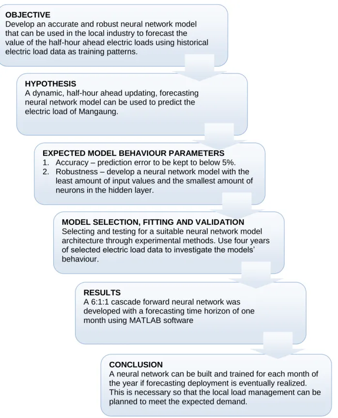
The research procedure of this project is represented by the flowchart in Figure 1.1

Figure 1.1: Research phases during execution of the project CONCLUSION

A neural network can be built and trained for each month of the year if forecasting deployment is eventually realized. This is necessary so that the local load management can be planned to meet the expected demand.

RESULTS

A 6:1:1 cascade forward neural network was developed with a forecasting time horizon of one month using MATLAB software

MODEL SELECTION, FITTING AND VALIDATION

Selecting and testing for a suitable neural network model architecture through experimental methods. Use four years of selected electric load data to investigate the models‟ behaviour.

EXPECTED MODEL BEHAVIOUR PARAMETERS

1. Accuracy – prediction error to be kept to below 5%. 2. Robustness – develop a neural network model with the

least amount of input values and the smallest amount of neurons in the hidden layer.

HYPOTHESIS

A dynamic, half-hour ahead updating, forecasting neural network model can be used to predict the electric load of Mangaung.

OBJECTIVE

Develop an accurate and robust neural network model that can be used in the local industry to forecast the value of the half-hour ahead electric loads using historical electric load data as training patterns.

5

1.3 Structure of this thesis

The essential layout of this project is shown in Figure 1.2

Figure 1.2: Layout of the thesis

An introduction to electric load forecasting theory with specific reference to short term load forecasting opens Chapter 2. The different shapes of load curves in a typical load pattern, planned load shedding, and a blackout are compared. Neural network theory with reference to the backpropagation and cascade correlation

Chapter 1 - Introduction

Chapter 2 - Literature review

Chapter 3 - Methology

Chapter 4 - Results

6

model, Levenberg-Marquardt minimization training algorithm and performance validation are also considered.

Since the aim of the project was not to investigate the mathematical theory behind neural networks, but its implementation in a working load forecasting model, little theory in this regard was covered. Only those aspects which influence the load forecasting model were identified.

The feedforward and the cascade forward neural network models were chosen for comparison according to:

 their architecture;

 backpropagation and Levenberg-Marquardt training algorithms;

 and performance using the mean absolute percentage error as a benchmark.

Extensive tests were done for three months of the year: May, June and July, for the three running years 2007, 2008 and 2009, to obtain a suitable model. This process is described extensively in Chapter 3.

Chapter 4 provides an exposition of how the final 6:1:1 neural cascade forward network was trained and its forecasting potential evaluated for the three months of the year: May, June and July, for the three running years 2007, 2008 and 2009. Evaluation was done using the mean absolute percentage error (MAPE) and correlation coefficients to measure and evaluate this cascade networks‟ performance. The MAPE, Daily Peak MAPE and linear regression plots, using July 2009 as a case study, are discussed in more detail. All these results are presented in this chapter.

7

CHAPTER 2 LITERATURE REVIEW 2.1 Electric load forecasting

Numerous books have been written about electric machinery, transmission systems and the protection technology needed to produce and deliver electric power. In comparison, little has been recorded about electric load forecasting. A forecast is a prediction of some future event. The importance of forecasting lies in the prediction of changes in load behaviour, which has a significant effect on various types of planning and decision-making processes in power systems operations and financial management.

Despite the large range of problem situations that involve forecasts, there are only two broad types of forecasting techniques: qualitative methods and quantitative methods.

Qualitative forecasts are often used in situations where there is little or no historical data on which to base the forecast. Quantitative forecasting techniques apply historical data to a forecasting model. The model recognizes patterns in the historical data and expresses a linear or non-linear relationship between the previous and current values of the data. Then the model projects the recognized data patterns into the future. The three most widely used Quantitative forecasting models are regression models, smoothing models and time series models [32, p.4]. Forecasting electric load curves are dependent on the assembly of historical load data so it will fall in the category of quantitative forecasting.

2.1.1 Forecasting the load curves

Normally, electric load curves alternate with time from a slow random swing to rapidly repeated pulses through daily, weekly, monthly, and annual cycles, creating continuously varying load curves from season to season. The

8

predictability of these load curves can be modeled with a wide range of roughly defined forecasting time periods, which includes:

Long term forecasting

The forecasting of bulk power for periods, years into the future. Usually, only peak loads are predicted.

Medium term load forecasting

The forecasting of bulk power for periods six months to one year ahead. Usually peak loads are forecasted and sometimes off-peak load values are also considered.

Short term load forecasting

This refers to much less than a “year ahead” forecast, and occasionally to a “one day ahead” forecast. The short term load forecasts differ from their long term counterparts in that peak forecasts assume less importance than forecasts at specific times; e.g., hour by hour forecasts will assume greater importance.

Load forecasting, especially Short Term Load Forecasting (STLF), is dependent on a combined load made up of different components. As an example, the load requirements can be decomposed into residential, industrial and commercial components [12, p.273] where the:

 Residential demand is proportional to a change in daily temperature;  Industrial loads are sensitive to economic and political factors; and the  Commercial demand is sensitive to the “day of the week” and occasional

holidays [22, p.302].

2.1.2 Quantitative short term load forecasting using time series data with a neural network model

Forecasting is usually based on identifying, modeling, and extrapolating the patterns found in historical data. Because historical data do not change dramatically very quickly, statistical methods, e.g. neural networks, are useful for short term forecasting [16, p.302].

9

It should be noted that power system transients such as sudden overloads due to short circuits, line harmonics or blackouts cannot be predicted with a forecasting model.

Most forecasting problems involve the use of time series data [36], which are amongst the oldest methods applied in load forecasting [19, p.904]. An electric load pattern is principally a time series [3, p.2]. A time series can be described as a sequential set of hourly, daily, or weekly data measured over regular intervals. A time series forecasting takes an existing series of data xt-n…,xt-3, xt-2, xt-1, xt and forecasts the xt+1 data value where:

xt+1 is the target value of x that we are trying to model;

xt is the value of x for the previous observation where we use

x to indicate an observation and t to represent the index of the time period.

As mentioned in par. 2.1, quantitative forecasting techniques involve the use of time series data (historical) and a forecasting model, i.e. an artificial neural network capable of representing complex nonlinear relationships. The model summarises patterns in the data and expresses a statistical relationship between previous and current values of the variable x, in this case. Patterns in the data can then be projected into the future, using this model [32, pp.1-5].

In neural network time series forecasting, two approaches are available in updating forecasting models over time: the rolling window approach and the sliding window approach.

The Rolling window approach uses a constant starting point and all the available data to train the neural network to anticipate the next value(s) and is not emphasized here. A disadvantage of this approach is that it is not very likely to give optimum results when the time series process is changing over time.

The Sliding window approach uses a changing starting point and a set of the latest observations to train the neural network to predict the next value(s). The sliding window approach adds a new training value and disregards the oldest one

10

BACKPROPAGATION

FORWARD PASS

from the training sample set which is used to update the neural model. The input sample set size, presented to the neural network, stays fixed as it slides forward with time.

It is not easy to determine an appropriate input sample set size that is useful for training the forecasting network. Too small a sample input set may restrict the power of the neural network to do proper forecasting by not adjusting the network parameters properly. However, the sliding window approach, with the changing starting point in the training sample set, is more suitable to contemplate changes occurring in the underlying process of the time series [33, pp.3-8].

As an example of a sliding window technique, Figure 2.1 shows a standard, trained back propagation neural network performing time series prediction using four equally time spaced input data points, sliding over the full training set of electric load data to predict the next output data point value [6].

Figure 2.1: Time series prediction using the “sliding window” approach

The rate at which the samples are taken will dictate the maximum resolution of the model. Once the network is trained with this set the same technique is used

11

with new data points to predict the future electric load. It is not always true that the model with the highest resolution will give the best forecasting performance. Currently, the available power generation capacity in South Africa is running in short supply. Load shedding needs to be applied frequently across the country to ensure the security of electricity supply, especially during the winter peak electricity demand of May, June and July. So, forecasting short term load can play an important role in power system operations decisions, taken when load shedding becomes a priority in the colder months of each year.

2.1.3 Load shedding

Occasionally, a misconception arises when discussing everyday load, load shedding and a blackout. One first has to understand the difference between a:

 typical load pattern,

 planned load shedding and a  blackout event

before considering the useful application of electric load forecasting.

A weekly load characteristic for Bloemfontein - July 2009 will be taken as an example to graphically illustrate the difference between the three concepts:

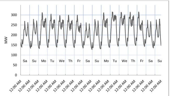
A typical load pattern

In Figure 2.2 it can be seen that the valleys in the daily pattern fluctuate little in magnitude and the base load floats at more or less 125 MW. The peak load levels for each day, indicating the Maximum Demand used for that day varies between 250 MW and 280 MW depending on the day-type one is looking at. An underlying repeating cyclic pattern, with random magnitudes at random periods, can be observed in the data.

12

Figure 2.2: A typical weekly load pattern

Planned Load shedding

Load shedding, also known as a rolling blackout, occurs when a power company cuts off electricity to selected areas to save power. This is a controlled way of rotating generating capacity. As an example, an area blackout can vary between two to six hours before the power is restored and the next area is cut off. Hospitals, airport control towers, police stations, and fire departments are often exempt from these rolling blackouts. One would be tempted to think that the load shedding curve would have the following shape, discussed next, which for practical reasons, are not predictable.

Example of an impracticable load shedding pattern

Figure 2.3 is a “clipped” version of the previous weekly pattern. It illustrates a hypothetical situation where the Maximum Demand is continuously controlled by cutting off the peak load to a maximum level of approximately 250 MW. In reality this type of load control is impractical to achieve.

0 50 100 150 200 250 300 L o ad M W

Weekly load curve

13

Figure 2.3: An impractical weekly load shedding pattern

Example of a realistic load shedding pattern

Figure 2.4 shows a practical situation. The load shedding curve closely follows the normal electric load demand pattern with a smaller peak magnitude in most places and can be presented to a load forecasting model for further research.

Figure 2.4: An actual weekly load shedding pattern 0 50 100 150 200 250 300 L o ad M W

Weekly load curve

Sat Sun Mon Tue Wed Thu Fri

0 50 100 150 200 250 300 L o ad M W

normal weekly load curve load shedding

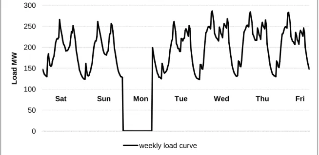
14 Example of a blackout event

Figure 2.5 shows a total power cut during a part of Sunday night and Monday. This type of uncontrolled power outage can affect a whole city or a big part of a country due to a network overload, act of Nature, terrorism or bad maintenance planning. If it lasts for more than a day or three, it can have a displeasing long term impact on transportation, water supply, communication, the local economy and the crime rate.

Figure 2.5: An example of a blackout occurring on a Monday

To summarise:

1. A typical daily load varies in a cyclic pattern and can be presented to a forecasting model.

2. Load shedding affects only a part of the populated area and:  can be classified as an example of short term load variation.

 on average the load drops to below its previous maximum daily peak load level values.

 a neural network can follow this type of change in load.

3. A blackout affects the whole city or region and it is totally unpredictable.

0 50 100 150 200 250 300 L o ad M W

weekly load curve

15

Economic and demographic factors in this region change very slowly over very long periods of time so medium- and long term forecasting is not applicable to critical factors like daily load shedding. However, short term load forecasting plays an important role when a decision is to be made during times of load shedding.

Some relatively recent forecasting models are available for research to predict the shape of electric load curves. The development of Artificial Intelligence (AI), especially Artificial Neural Networks (ANN) can be applied for research to model short term load forecasting.

Artificial neural networks have been extensively used as time series predictors; these are usually feed-forward networks that make use of a sliding window over the input data sequence. Using a combination of a time series and a neural network prediction method, the past events of the load data can be explored and used to train a neural network to predict the next load point.

There are many neural network training methods and architectures that can be used to model a forecasting problem, but only the applications and principles used in this investigation will be discussed next.

2.2 Some principles of artificial neural networks 2.2.1 Introduction

Artificial neural networks, “roughly” based on the architecture of the brain, are rising as an exciting new information-processing concept for AI systems. Their working mechanism is totally different from conventional computers in the following way:

 They do not need to be programmed, as they can learn from examples through training.

 They can produce correct outputs from noisy and incomplete data (fault tolerant), whereas conventional computers usually require correct data.

16

 If one or more neurons or communication lines are damaged, the network degrades „gracefully‟ (that is, in a progressive manner), unlike sequential computers which can fail catastrophically after isolated failures.

 They are economic to build and to train.

Due to these differences in working mechanisms, considerable interest have been created in the possibilities for applying neural networks in engineering, and have resulted in a great deal of research over the last few years. Some of the claimed advantages are exaggerated, but others are certainly proven, and neural networks are slowly becoming a standard technology for engineers [26, p.95], [2, p.31].

In the 1980‟s research in neural networks increased substantially because personal computers became widely available [55, p.41]. Two new mathematical tools were responsible for the rejuvenation of neural networks in the 1980s:

 The use of statistical mechanics explaining the operation of a certain class of network;

 The discovery of the back-propagation algorithm for training multi-layer perceptron networks.

These new developments recharged the interest in the field of neural networks.

2.2.2 Moving to artificial neural network structures

An artificial neural network consists of a number of very simple processors, also called neurons, which are analogous to the biological neurons in the brain. The neurons are connected by weighted links passing signals from one neuron to another.

The input signal is transmitted through the network neurons to its outgoing connection. Each neuron connection can split into a number of branches, the weighted links, to transmit the received signal. The links can amplify or weaken

17

Input signals Output

signals

each signal as it passes through, according to its allocated weight value. A simple network is illustrated in Fig 2.6.

Figure 2.6: Layout of a plain artificial neural network

More complex systems will have more layers of neurons with some having increased layers of input neurons and output neurons.

Next, the behaviour of a neural network is discussed by first showing the essential features of neurons and their weighted links. However, because our knowledge of neurons is incomplete and our computing power is limited, this mathematical model is a crude portrayal of real networks of neurons.

2.2.2.1 A general mathematical neuron model - the perceptron

A specific artificial mathematical neuron, the perceptron, is considered, based on McCulloch and Pitt‟s model. The perceptron is the simplest form of a neural network and consists of a single neuron with adjustable weighted links and an activation function called a “hard limiter”, sign- or a threshold function.

This perceptron-neuron, shown in Figure 2.7, computes the weighted sum of the input signals and adds the result to a bias value,



X that will be presented to the activation function. This activity is referred to as a linear combination.

18 X2 _Bias

∑



If the net input is less than a threshold value (e.g. zero on the x-axis), the neuron output is -1. But if the net input is greater than or equal to the zero threshold value on the x-axis, the neuron becomes activated and its output value, Y,

becomes +1.

This situation is referred to as the neuron having “fired”. The perceptron-neuron in Figure 2.7 uses the “sign” or “threshold” activation function.































0

0

X

if

1,

X

if

1,

Y

i

θ

n

1

i

i

w

i

x

X

Figure 2.7: A single layer, two input, linear threshold perceptron where X is the net input and Y is the neuron output

In Figure 2.7 it can be seen that the combination of the weighted links and the activation function are used to control the amplitude of the output. An activation function is a mathematical function used by a neural network to scale numbers to a specific range.

19

There are many activation functions that one can choose from and each one has its own special merits [5, p.44]. The four basic activation functions are discussed next.

2.2.2.1.1 Basic activation functions

Many different types of linear or nonlinear activation functions (or limiters) can be designed [18, pp.2-6]. Choosing the correct function depends on the particular problem to be solved. A basic reference model for the presentation of activation functions is shown in Figure 2.8 [7, p.21].

Heaviside Step function Sigmoid function Linear function Sign function

f

x

=

1, if x≥0

0, if x<0

f

x

=

1

1+e

f

x

=

x f

x

=

1, if x≥0

-1, if x<0

Figure 2.8: Four basic types of activation functions

1. The Heaviside step function and the Sign function are binary functions that hard limit the input to the function to either a 1 or a 0 for the binary type, and a -1 or a 1 for the bipolar type.

2. Sigmoid functions are the most commonly used function in the

construction of artificial neural networks [21, p.14]. They are also known as “squashing functions”, thought of as a slowly softened Sign function [17]. This type of function is nonlinear and therefore differentiable everywhere, causing greater weight change activity to take place for neurons where the output is less certain (i.e. close to 0.5 where the slope

X 0 Y -1 +1 0 _X Y -1 +1 X 0 Y -1 +1 0 Y -1 + 1 X

20

is the steepest) than those in which it is more certain (i.e. close to 0 or 1) [1, p.138]. This type of nonlinearity is very important, or else the input-output relationship of the network will be reduced to that of a single layer perceptron network [21, p.157]. Interestingly, artificial neurons containing sigmoidal functions resemble a type of biological neuron found in the brain [56, p.5].

3. The Linear limiter is a continuous function where the output purely reflects the input. This function is usually combined with other functions for specific tasks at hand, i.e. linear networks.

2.2.2.2 Connecting perceptrons into structures called networkarchitectures

A single perceptron is not very useful because of its limited mapping ability. Multiple perceptrons can be connected as building blocks of a larger, much more practical structure called an artificial neural network or a complex nonlinear mapping tool. This type of neural net can deal with complex nonlinearities in a fairly general way [56, p. 2]. Many kinds of neural networks exist today and variations of older structures are invented regularly [47, p.14].

There is a large variety of neural network structures to choose from. The selection or design of a particular network depends on the uniqueness of the intended application. The following aspects should be given careful consideration:

 How well can the network model the system?

 How efficient can the network structure and parameter values be adapted?  Amount of accuracy required;

 Overall problem complexity;  System stability;

 Is off-line or on-line implementation required?

Other important questions to consider when setting up a neural network are:  Should the network be fully or partially connected?

21

Input layer Hidden layer Output layer

Back propagation training: Adapting the layer weights/bias using the output error data values until a predetermined value is reached.

Direction of flow of the input data

 How many layers are needed?

 How many neurons should be in each layer?

 What type of activation function should be used [23, p.28]?

 Can one obtain a sufficient historical data set from the system to be predicted to train the neural network?

Once the network connection structure has been decided upon, the following step would be to adjust the network biases and weights by a suitable training method so that the network input/output relationship is very close to that of the system to be modeled.

The well-known feedforward connection structure will be discussed next. The term “Feedforward” means that the input signal moves from the input to the output layer.

2.2.2.3 Multilayer feedforward network connection structure

All feedforward neural networks have an input layer and an output layer, but the number of hidden layers may vary. This class of layered network has one or more hidden layers presented in the three-layer net, as shown in Figure 2-9.

22

This network structure is referred to as a 3:4:2 network because it has 3 inputs, 4 hidden neurons and 2 output neurons. This network is said to be fully connected in the sense that every neuron in each layer is connected to every other neuron in the next forward layer.

If some of the communication links between the neurons are not part of the designed network then it is referred to as being partially connected. The “hidden layers” can communicate backwards with the input source nodes and forward with the output layer in some determined manner. By adding a hidden layer or two, the neural net can handle some highly nonlinear problems that would be difficult to describe mathematically.

The most efficient number of hidden layers depends in a complex way on the:  number of input and output units;

 number of training cases;

 amount of noise in the input signal;

 complexity of the function or classification to be learned;  network‟s architecture;

 type of hidden layer activation function;  training algorithm;

 regularisation.

2.2.3 Training a neural network

Training is as essential for a neural network as programming is for a computer to function properly. The activation function of a neuron is fixed when the network is set up and the set of signals to which it is supposed to react is fixed. During the training phase, the only adjustment that can be made to individual neuron‟s input/output behaviour is to its own input weights and biases [43]. Therefore, the

23

correct choice of a learning algorithm is an important issue in network development.

One of the problems that can occur during training is over-learning or over-fitting. The desire for the neural network is to provide a correct mapping of the test data and maintain the ability to generalize for new data. The results of over-fitting can already be visible in the test stage [24, p.274].

A critical goal during training is to find a network large enough to learn the task but small enough to generalize [20, p.53].

In this project, the neural network must be able to learn a model of the electric load which it will be predicting. It must be able to maintain the model adequately and reliably when used to predict real load variations so as to achieve the particular goals of the application of interest [21, p.24].

For different network structures, different training algorithms have been developed. Neural nets are classified according to their corresponding training algorithms:

 fixed weight networks;  supervised networks; and  unsupervised networks.

No learning is required for a fixed weight network, so the common training algorithms are supervised and unsupervised learning [54, p.249].

2.2.3.1 Supervised training

The prevailing current of thought of artificial neural network development has been focused on supervised learning networks. To commence learning this type of network, data needs to be gathered and consists of pairs of input/output training sets. First the training sets are presented to the network. Then, through comparison of the actual and desired response (the error) at the output stage,

24

adjustments of the weights and biases of the whole parameter space are made. In this way, learning or proper classification is facilitated with the help of a teacher, as shown in Figure 2.10 [37, p.14].

Figure 2.10: Block diagram of learning with a teacher

The special quality of a network exists in the values of the bias and weights between any two of its neurons, so we need a method of adjusting the bias and weights to solve a particular mathematical problem. For feedforward networks, the most common training algorithm is called Back Propagation (BP). A BP network learns by example, that is, we must provide a learning set that consists of pairs of data sets (input examples and the known-correct outputs for each case). So, we use these input-output examples to show the network what type of performance is expected, and the BP algorithm adjusts the weights and biases in the network after the input/output pairs are compared.

2.2.3.1.1 Supervised training using backpropagation

The backpropagation training algorithm was first described by Rumelhart and McClelland [42] in 1986; it was the first convenient method for training neural networks. The original procedure used the gradient descent algorithm to adjust the weights toward convergence, using the gradient (the direction in which the performance index will decrease most rapidly). The term “backpropagation” or

+ _ Actual response Desired response Error signal Learning system Teacher Preferred data Training data

25

“backprop” is often used to indicate a neural network learning algorithm using the gradient descent algorithm.

To make practical forecasts for this work, the different neural networks were trained using appropriate data series sets. Training examples in the form of (input, target) pairs of vectors are extracted from the data series. The input and target vectors are equal in size to the number of network inputs and outputs, in the order mentioned.

For every training example presented to the network, the algorithm follows a sequence of steps to adapt each neuron‟s weight and bias values before the following training example is presented to it. The sequence is as follows:

1. The learning procedure works in small adjustable incremental steps: one of the example pairs is presented to the network in a forward pass, and the network produces some outputs based on the present state of its bias and weights (initially, the outputs will be random because the values of the biases and weights were chosen randomly). The output of the first layer becomes the input to the second layer and so forth until a final value is available at the output layer, the network output.

2. The final output value is compared to the target value. This is the difference (the error) between the desired value (the target that the network will need to learn) and the actual network output value obtained from the input training examples in 1.

3. This error is backpropagated from the output layer to the first hidden layer through the network, calculating the gradient (vector of derivatives) of the change in error with respect to the changes in weight values.

4. All the network neuron weights and biases in proportion to the error are updated.

5. Steps 1 to 4 is repeated until the difference, measured using a performance index (e.g. the mean square error) has been reduced to a preset value.

26

Each complete cycle of these steps is called an epoch. Training will end when a maximum number of epochs or a network output error limit is reached as programmed by the network user.

Training can be time consuming, depending on the number of example sets, network size and topology, epoch- and error limits.

Because the error information is propagated backward through the network, this type of training method is called backward propagation. A mathematical description of the above sequence will be explained next.

Backpropagation algorithm

Kindly abusing the much quoted work of Hagan, Demuth and Beale, “Neural Network Design” [18, pp.11-7 to 11-13], a brief explanation of a more accepted approach to the backpropagation training algorithm is shown where the notation from Hagan is represented as follows:

Scalars: small italic letters…a, b, c

Vectors: small bold letters…a, b, c Matrices: capital BOLD letters…A, B, C

Vector: column of numbers.

27

Figure 2.11: Two layer network shown in abbreviated notation where the

output vector of the first (hidden layer), a1,becomes the input vector to the

second (output) layer

Consider an example of a multilayer feedforward network as in Figure 2.11.

Step 1 - Forward propagation

For an M layer network the system equations in matrix form are given by

a0_{=p, (2.1)}

for the input layer where the input vector elements am+1enter the network through the weight matrix W and

am+1_{= f} m+1 _Wm+1_am_+bm+1 _{for m = 0,1,…,M-1, (2.2)}

is the transfer function vector for the output layer, so that the last network layer outputs, considered as the network outputs, are:

a = aM_{, (2.3)}

where

𝐩= network input vector and

n1 p W1 b1 +1 f 1 n 2 a1 _W2 b2 +1 f 2 a2 a1_=f1_(w1_p+b1_{) a}2_=f2_(w2_a1_+b2₎ a2 _{= f}2 _(w2 _{( f}1_(w1_p+b1 _{) ) + b}2 ₎ a0_=p

28

a0,a1…a𝑀= network output vectors

Step 2 - Backpropagation

The task of the network is to learn associations using a training set of prototype input-output examples:

p₁,t₁ , p₂,t₂ , …, p_q,t_q , (2.4)

where pq is a network input and tq is the matching target output. For each input pq

applied to the network, the network output (a) will be compared to the target output (t). The difference will be the error (e), used to calculate the performance index F(x) using the mean square error (MSE):

F(x) = E [ e2 _{] = E [ (t – a )}2 _{]. (2.5)}

Where x is the vector of network weights and biases and E[ ] donates the

expected value where the expectation is taken over all sets of input-target pairs. The algorithm adjusts the network parameters to minimize the MSE.

For a multiple output network it generalizes to vectors

F(x) = E [eT_{e] = E [(t - a)} T _{(t - a)]. (2.6)}

So the approximate MSE (Single sample) or performance index for the network is

𝐹 x = 𝐭 k − 𝐚 k T 𝐭 k − 𝐚 k = 𝐞T _{k 𝐞 k (2.7)}

where the expectation of the squared error is replaced by the squared error at iteration k.

The steepest descent algorithm searches the parameter space (adjusting the weights and biases) in order to reduce the mean square error 𝐹 x . Updating the weights at each iteration k is

29

w_i,jm _{k+1 = w}

i,j m k – α_{∂ w}∂ F

i,jm (2.8)

and the biases is

b_i,jm _{k+1 = b} i,j

m _{k – α} ∂ F

∂ b_im (2.9)

Where α is the learning rate which determines the length of the step in the search direction to minimize 𝐹 x .

The error is an indirect function of the weights in the hidden layer, so the chain rule of calculus is used to compute the partial derivatives. The derivatives in Eq. 2.8 and Eq. 2.9 are written as:

_{∂ w}∂ F i,j m= ∂ F ∂ 𝑛_im × ∂𝑛_𝑖𝑚 ∂ w_i,jm (2.10) ∂ F ∂ b_im= ∂ F ∂ n_im × ∂𝑛_𝑖𝑚 ∂ b_im (2.11)

Since the net input to a layer m is a function of the weights and bias in that layer:

𝑛_𝑖𝑚 _{= 𝑤}

𝑖,𝑗𝑚𝑎𝑗𝑚−1 𝑠𝑚 −1

𝑗 =1 + 𝑏𝑖𝑚 (2.12)

The second term in Eq. 2.10 and Eq. 2.11 will be ∂𝑛_𝑖𝑚 ∂ w_i,jm= 𝑎𝑗 𝑚 −1 _(2.13) And ∂𝑛𝑖 𝑚 ∂ b_im= 1 (2.14)

Specify s as the sensitivity of the performance index 𝐹 to changes in the i th element of the net input at layer m:

30

𝑠_𝑖𝑚 ≡ _{∂ 𝑛}∂ F

i

m (2.15)

Then Eq. 2.10 and Eq. 2.11 can be reduced to

∂ F ∂ w_i,jm= 𝑠𝑖 𝑚_𝑎 𝑗𝑚−1 (2.16) _{∂ b}∂ F i m= 𝑠𝑖𝑚 (2.17)

This algorithm can now be expressed as

𝑤_𝑖,𝑗𝑚 _{𝑘 + 1 = 𝑤}

𝑖,𝑗𝑚 𝑘 −∝ 𝑠𝑖𝑚𝑎𝑗𝑚−1 (2.18)

For the weight and

𝑏_𝑖𝑚 _{𝑘 + 1 = 𝑏}

𝑖𝑚 𝑘 −∝ 𝑠𝑖𝑚 (2.19)

For the bias

The next step is to propagate the sensitivities backward through the network to compute the gradient:

Compute the sensitivity 𝑠𝑚 which requires another application of the chain rule. This part of the routine has led to the term “backpropagation”. It describes a “repetitive” relationship in which the sensitivity 𝑠𝑚 _{at layer m is calculated from}

the sensitivity 𝑠𝑚 +1 at layer m+1. To derive this relationship for the sensitivities, the following Jacobian matrix is used:

𝜕𝑛 𝑚 +1 𝜕𝑛𝑚 = 𝜕𝑛₁𝑚 +1 𝜕𝑛₁𝑚 𝜕𝑛₁𝑚 +1 𝜕𝑛₂𝑚 ⋯ 𝜕𝑛1𝑚 +1 𝜕𝑛_𝑠𝑚𝑚 𝜕𝑛2𝑚 +1 𝜕𝑛1𝑚 ⋮ 𝜕𝑛_{𝑠𝑚 +1}𝑚 +1 𝜕𝑛₁𝑚 𝜕𝑛2𝑚 +1 𝜕𝑛2𝑚 ⋮ 𝜕𝑛_{𝑠𝑚 +1}𝑚 +1 𝜕𝑛₂𝑚 ⋯ 𝜕𝑛₁𝑚 +1 𝜕𝑛_𝑠𝑚𝑚 ⋮ 𝜕𝑛_{𝑠𝑚 +1}𝑚 +1 𝜕𝑛_𝑠𝑚𝑚 (2.20)

To find an expression for this matrix the following i,j elements of the matrix is considered:

31 𝜕𝑛_𝑖𝑚 +1 𝜕𝑛_𝑗𝑚 = 𝜕 𝑠𝑚_𝑙=1𝑤_𝑖,𝑙𝑚 +1𝑎_𝑙𝑚+𝑏_𝑖𝑚 +1 𝜕𝑛_𝑗𝑚 𝑤_𝑖,𝑗𝑚+1×𝜕𝑎𝑗𝑚 𝜕𝑛_𝑗𝑚 = 𝑤𝑖,𝑗 𝑚+1_×𝜕𝑓𝑚(𝑛𝑗𝑚) 𝜕𝑛_𝑗𝑚 = 𝑤𝑖,𝑗 𝑚 +1_{× 𝑓}𝑚_(𝑛 𝑗 𝑚₎ where 𝑓𝑚_(𝑛 𝑗 𝑚_{) =} 𝜕𝑓𝑚(𝑛𝑗𝑚) 𝜕𝑛_𝑗𝑚 (2.21)

So the Jacobian matrix can be written as 𝜕𝒏_𝜕𝒏𝑚 +1_𝑚 = 𝑾𝑚+1 × 𝐹 𝑚 𝒏𝑚 ) (2.22) where 𝐹 𝑚 𝒏𝑚 ) = 𝑓𝑚(𝑛1𝑚) 0 ⋯ 0 0 ⋮ 0 𝑓 𝑚_(𝑛 2𝑚) ⋮ 0 ⋯ 0 ⋮ 𝑓 𝑚_(𝑛 𝑠𝑚 𝑚 ₎ (2.23)

Using the chain rule in matrix form, the recurrence relationship for the sensitivity can be written as:

𝒔𝑚 ₌ 𝜕𝐹 𝜕𝐧𝑚 = 𝜕𝐧𝑚 +1 𝜕𝐧𝑚 𝑇 _𝜕𝐹 𝜕𝐧𝑚 +1 = F 𝑚 𝐧𝑚 𝐖𝑚+1 𝑇 𝜕𝐹 𝜕𝐧𝑚 +1 = F 𝑚 𝒏𝑚 𝑾𝑚+1 𝑇𝒔𝑚+1 (2.24)

The sensitivities are computed by starting at the last layer, and then propagating backwards through the network to the first layer.

𝒔𝑀 _{→ 𝒔}𝑀−1 _{→ ⋯ → 𝒔}2 _{→ 𝒔}1

32

The starting point, 𝒔𝑚, for the recurrence relation of Eq. 2.23 is obtained at the final network layer:

𝑠_𝑖𝑀 =_𝜕𝑛𝜕𝐹 𝑖 𝑀 = 𝜕 𝒕−𝒂 𝑇 𝒕−𝒂 𝜕𝑛_𝑖𝑀 = 𝜕 𝑆𝑀𝑗 =1 𝑡𝑗−𝑎𝑗 2 𝜕𝑛_𝑖𝑀 = −2 𝑡𝑖 − 𝑎𝑖 𝜕𝑎𝑖 𝜕𝑛_𝑖𝑀 (2.25)

So that from Eq. 2.21

𝑠_𝑖𝑀 _{= −2 𝑡}

𝑖− 𝑎𝑖 𝑓 𝑀(𝑛𝑗𝑀)

Expressed in matrix form as

sM = -2 𝐅 M nM t - a (2.26)

Sm_=Fm _nm _Wm+1 T_sm+1_{, for m = M - 1,…, 2,1 (2.27)}

Step 3 - Weight update

Backpropagation learning updates the network weights and biases in the direction in which the performance function diminishes most rapidly – the negative of the gradient. One iteration of this algorithm can be written as

Wm k+1 = Wm k - ∆Wm k , (2.28)

Where the change in weight is

∆Wm k = - α sm am-1 T. (2.29)

and

bm k+1 = bm k - ∆bm k , (2.30)

33

∆bm k = - α sm. (2.31)

The iteration is continued until the difference between the network response and the target function reaches some desired level set by the computer programmer.

2.2.3.2 Drawbacks of backpropagation training The error performance surface

The mean square error (MSE) performance surface for a single-layered linear network is a quadratic function with only one single stationary point and constant curvature. Therefore, this training algorithm is guaranteed to converge to a solution that minimizes the MSE if the learning rate, α, is not too large.

The performance surface curvature for a multilayer nonlinear network, not a quadratic function, can vary widely in different regions of the weight parameter space. It would then be difficult to choose an appropriate learning rate for the steepest descent algorithm. For a flat surface, (a sigmoid transfer function output for large inputs saturates) a large learning rate would be suitable whereas for a region where the curvature is high, a smaller learning rate would be required. Another feature of this error surface is the existence of many local minimum points. The steepest descent algorithm would effectively stop at a local minimum or even if the surface gradient is close to zero.

Also, if a multilayer network has two local minimum points with the same value of the squared error, the origin (0, 0) of the parameter space tends to be a saddle point for the performance surface. This might happen if the initial values of the weights and biases are set to zero.

In conclusion, the initial parameters should then be chosen to be small random values [18, p.12-5].

34

Convergence to the minimum error

In some instances the entire training set is presented to the network (batch training) before the parameters are updated. Slow or fast convergence can occur due to sudden changes in the curvature of the surface over the path of the steepest descent‟s trajectory towards the minimum error.

For example, changing the learning rate to speed up the convergence when it is traversing a flat section could make the algorithm‟s trajectory unstable when it reaches a steeper portion of the performance surface. This divergence or oscillations across the error surface can be smoothed out using a low pass “momentum” filter [18, p12-8].

Improving the gradient descent algorithm

Momentum

If one could filter the steepest descent‟s trajectory by averaging the updates to the parameters, this might smooth out the oscillations and produce a stable trajectory. This is done by adding a low pass filter termed momentum.

Adding a momentum coefficient γ tends to speed up convergence when the trajectory is moving in a steady direction. The larger the value ofγ, the more “momentum” the trajectory has.

When the momentum modification is added to the parameter updates for the steepest descent backpropagation, Eq.(2.29) and Eq.(2.31) change to:

∆Wm _{k = γ∆W}m _{k - 1 – 1 - γ α s}m _am-1 T_{, (2.32)}

And

∆bm k = γ∆bm k - 1 – 1 - γ α sm. (2.33)