and Data Management, 3rd Edition
A Guide for SPSS and SAS
®Users
Chicago, IL 60606-6412 Tel: (312) 651-3000 Fax: (312) 651-3668
SPSS is a registered trademark and the other product names are the trademarks of SPSS Inc. for its proprietary computer software. No material describing such software may be produced or distributed without the written permission of the owners of the trademark and license rights in the software and the copyrights in the published materials.
The SOFTWARE and documentation are provided with RESTRICTED RIGHTS. Use, duplication, or disclosure by the Government is subject to restrictions as set forth in subdivision (c) (1) (ii) of The Rights in Technical Data and Computer Software clause at 52.227-7013. Contractor/manufacturer is SPSS Inc., 233 South Wacker Drive, 11th Floor, Chicago, IL 60606-6412. General notice: Other product names mentioned herein are used for identification purposes only and may be trademarks of their respective companies.
SAS is a registered trademark of SAS Institute Inc.
Windows is a registered trademark of Microsoft Corporation. Microsoft® Access, Microsoft® Excel, and Microsoft® Word are products of Microsoft Corporation.
DataDirect, DataDirect Connect, INTERSOLV, and SequeLink are registered trademarks of DataDirect Technologies. Portions of this product were created using LEADTOOLS © 1991–2000, LEAD Technologies, Inc. ALL RIGHTS RESERVED. LEAD, LEADTOOLS, and LEADVIEW are registered trademarks of LEAD Technologies, Inc.
Portions of this product were based on the work of the FreeType Team (http://www.freetype.org).
A portion of the SPSS software contains zlib technology. Copyright © 1995–2002 by Jean-loup Gailly and Mark Adler. The zlib software is provided “as-is,” without express or implied warranty. In no event shall the authors of zlib be held liable for any damages arising from the use of this software.
A portion of the SPSS software contains Sun Java Runtime libraries. Copyright © 2003 by Sun Microsystems, Inc. All rights reserved. The Sun Java Runtime libraries include code licensed from RSA Security, Inc. Some portions of the libraries are licensed from IBM and are available athttp://oss.software.ibm.com/icu4j/. Sun makes no warranties to the software of any kind. Sax Basic is a trademark of Sax Software Corporation. Copyright © 1993–2004 by Polar Engineering and Consulting. All rights reserved.
SPSS Programming and Data Management, 3rd Edition: A Guide for SPSS and SAS Users Copyright © 2006 by SPSS Inc.
All rights reserved.
Printed in the United States of America.
No part of this publication may be reproduced, stored in a retrieval system, or transmitted, in any form or by any means—electronic, mechanical, photocopying, recording, or otherwise—without the prior written permission of the publisher.
1 2 3 4 5 6 7 8 9 0 09 08 07 06 ISBN 1-56827-374-6
Experienced data analysts know that a successful analysis or meaningful report often requires more work in acquiring, merging, and transforming data than in specifying the analysis or report itself. SPSS contains powerful tools for accomplishing and automating these tasks. While much of this capability is available through the graphical user interface, many of the most powerful features are available only through command syntax. With release 14.0.1, SPSS makes the programming features of its command syntax significantly more powerful by adding the ability to combine it with a full-featured programming language. This book offers many examples of the kinds of things that you can accomplish using SPSS command syntax by itself and in combination with the Python programming language.
Using This Book
The contents of this book and the accompanying CD are discussed in Chapter 1. In particular, see the section “Using This Book” if you plan to run the examples on the CD. The CD also contains additional command files, macros, and scripts that are mentioned but not discussed in the book and that can be useful for solving specific problems.
This edition has been updated to include numerous enhanced data management features introduced in SPSS 14.0. Many examples will work with earlier versions, but some examples rely on features not available prior to SPSS 14.0. All of the Python examples require SPSS 14.0.1 or later.
For SAS Users
If you have more experience with SAS than with SPSS for data management, see Chapter 19 for comparisons of the different approaches to handling various types of data management tasks. Quite often, there is not a simple command-for-command relationship between the two programs, although each accomplishes the desired end.
examples here and in SPSS Developer Central, as well as that of Raynald Levesque, whose examples formed the backbone of earlier editions and remain important in this edition. We also wish to thank Stephanie Schaller, who provided many sample SAS jobs and helped to define what the SAS user would want to see, as well as Marsha Hollar and Brian Teasley, the authors of the original chapter “SPSS for SAS Programmers.”
A Note from Raynald Levesque
It has been a pleasure to be associated with this project from its inception. I have for many years tried to help SPSS users understand and exploit its full potential. In this context, I am thrilled about the opportunities afforded by the Python integration and invite everyone to visit my site atwww.spsstools.netfor additional examples. And I want to express my gratitude to my spouse, Nicole Tousignant, for her continued support and understanding.
Raynald Levesque
1
Overview
1
Using This Book . . . 1
Documentation Resources . . . 2
Part I: Data Management
2
Best Practices and Efficiency Tips
5
Working with Command Syntax . . . 5Creating Command Syntax Files . . . 5
Running SPSS Commands . . . 6
Syntax Rules . . . 7
Customizing the Programming Environment . . . 8
Displaying Commands in the Log . . . 8
Displaying the Status Bar in Command Syntax Windows . . . 9
Protecting the Original Data . . . 10
Do Not Overwrite Original Variables. . . 11
Using Temporary Transformations . . . 11
Using Temporary Variables . . . 12
Use EXECUTE Sparingly . . . 14
Lag Functions . . . 14
Using $CASENUM to Select Cases. . . 16
MISSING VALUES Command . . . 17
WRITE and XSAVE Commands . . . 17
Using Comments. . . 17
Using SET SEED to Reproduce Random Samples or Values . . . 18
3
Getting Data into SPSS
23
Getting Data from Databases . . . 23
Installing Database Drivers . . . 23
Database Wizard . . . 25
Reading a Single Database Table . . . 25
Reading Multiple Tables. . . 27
Reading Excel Files. . . 30
Reading a “Typical” Worksheet . . . 31
Reading Multiple Worksheets . . . 33
Reading Text Data Files. . . 36
Simple Text Data Files . . . 37
Delimited Text Data . . . 38
Fixed-Width Text Data . . . 42
Text Data Files with Very Wide Records . . . 47
Reading Different Types of Text Data . . . 48
Reading Complex Text Data Files. . . 49
Mixed Files . . . 50
Grouped Files . . . 51
Nested (Hierarchical) Files . . . 54
Repeating Data . . . 59
Reading SAS Data Files . . . 61
Reading Stata Data Files . . . 63
Working with Multiple Data Sources. . . 65
Merging Data Files . . . 69
Merging Files with the Same Cases but Different Variables . . . 69
Merging Files with the Same Variables but Different Cases . . . 73
Updating Data Files by Merging New Values from Transaction Files . . . . 77
Aggregating Data . . . 79
Aggregate Summary Functions . . . 81
Weighting Data. . . 82
Changing File Structure . . . 84
Transposing Cases and Variables. . . 85
Cases to Variables . . . 86
Variables to Cases . . . 89
5
Variable and File Properties
95
Variable Properties . . . 95Variable Labels . . . 98
Value Labels . . . 98
Missing Values . . . 99
Measurement Level . . . 100
Custom Variable Properties . . . 100
Using Variable Properties As Templates . . . 102
File Properties . . . 103
6
Data Transformations
105
Recoding Categorical Variables . . . 105Random Value and Distribution Functions . . . 111
String Manipulation . . . 112
Changing the Case of String Values . . . 113
Combining String Values . . . 113
Taking Strings Apart . . . 114
Working with Dates and Times . . . 118
Date Input and Display Formats . . . 119
Date and Time Functions . . . 122
7
Cleaning and Validating Data
129
Finding and Displaying Invalid Values . . . 129Excluding Invalid Data from Analysis . . . 132
Finding and Filtering Duplicates . . . 133
Data Validation Option . . . 136
8
Conditional Processing, Looping, and
Repeating
139
Indenting Commands in Programming Structures . . . 139Conditional Processing . . . 140
Conditional Transformations . . . 140
Conditional Case Selection . . . 143
Simplifying Repetitive Tasks with DO REPEAT . . . 144
ALL Keyword and Error Handling . . . 147
Vectors. . . 147
Indexing Clauses . . . 152
Nested Loops . . . 153
Conditional Loops . . . 155
Using XSAVE in a Loop to Build a Data File. . . 156
Calculations Affected by Low Default MXLOOPS Setting . . . 158
9
Exporting Data and Results
161
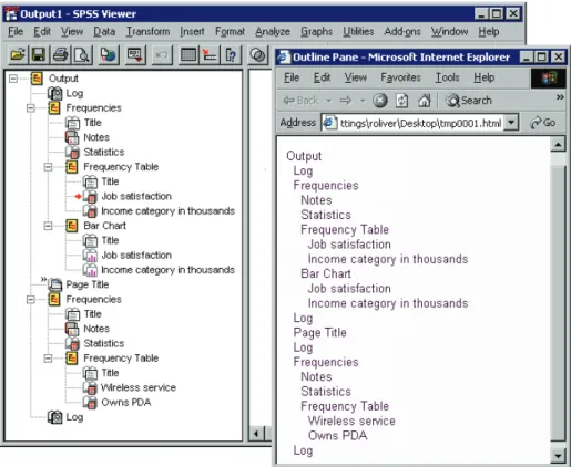
Output Management System. . . 161Using Output as Input with OMS . . . 162
Adding Group Percentile Values to a Data File . . . 162
Bootstrapping with OMS . . . 166
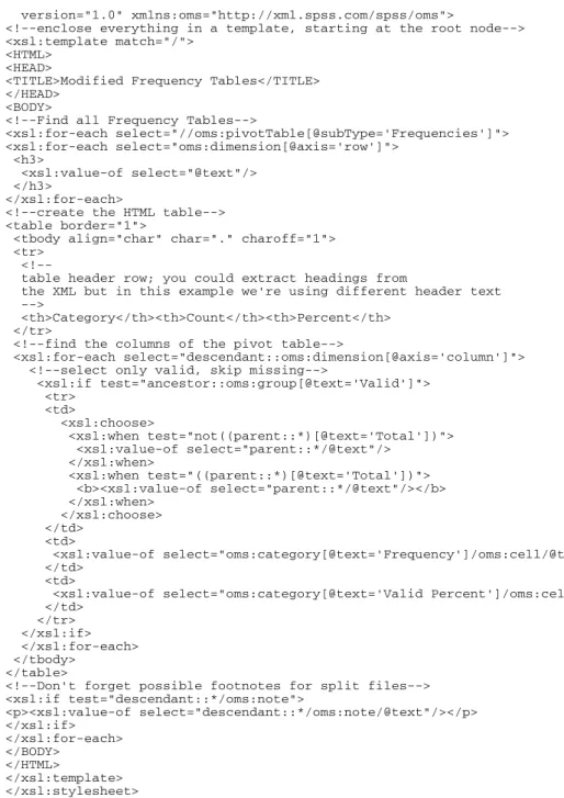
Transforming OXML with XSLT . . . 171
“Pushing” Content from an XML File . . . 172
“Pulling” Content from an XML File . . . 175
Positional Arguments versus Localized Text Attributes. . . 184
Layered Split-File Processing. . . 185
Exporting Data to Other Applications and Formats . . . 186
Saving Data in SAS Format . . . 186
Saving Data in Stata Format. . . 187
Saving Data in Excel Format. . . 189
Writing Data Back to a Database . . . 189
Saving Data in Text Format. . . 192
Exporting Results to Word, Excel, and PowerPoint . . . 192
Introduction . . . 193
Basics of Scoring Data . . . 194
Command Syntax for Scoring. . . 194
Mapping Model Variables to SPSS Variables . . . 196
Missing Values in Scoring . . . 196
Using Predictive Modeling to Identify Potential Customers . . . 197
Building and Saving Predictive Models . . . 197
Commands for Scoring Your Data. . . 204
Including Post-Scoring Transformations . . . 205
Getting Data and Saving Results . . . 206
Running Your Scoring Job Using the SPSS Batch Facility . . . 207
Part II: Programming with SPSS and Python
11 Introduction
211
12 Getting Started with Python Programming in
SPSS
215
The spss Python Module. . . 216Submitting Commands to SPSS. . . 217
Dynamically Creating SPSS Command Syntax. . . 219
Capturing and Accessing Output. . . 220
Python Syntax Rules . . . 222
Mixing Command Syntax and Program Blocks . . . 224
Handling Errors. . . 227
13 Best Practices
233
Creating Blocks of Command Syntax within Program Blocks. . . 233
Dynamically Specifying Command Syntax Using String Substitution . . . 234
Using Raw Strings in Python . . . 237
Displaying Command Syntax Generated by Program Blocks . . . 238
Handling Wide Output in the Viewer . . . 239
Creating User-Defined Functions in Python . . . 239
Creating a File Handle to the SPSS Install Directory . . . 241
Choosing the Best Programming Technology . . . 242
Using Exception Handling in Python . . . 243
Debugging Your Python Code . . . 247
14 Working with Variable Dictionary Information 251
Summarizing Variables by Measurement Level . . . 253Listing Variables of a Specified Format . . . 254
Checking If a Variable Exists . . . 256
Creating Separate Lists of Numeric and String Variables. . . 257
Using Object-Oriented Methods for Retrieving Dictionary Information. . . 258
Getting Started with the VariableDict Class . . . 259
Defining a List of Variables between Two Variables . . . 262
Identifying Variables without Value Labels . . . 264
Retrieving Definitions of User-Missing Values . . . 268
15 Getting Case Data from the Active Dataset
273
Using the Cursor Class . . . 273
Reducing a String to Minimum Length. . . 277
Using the spssdata Module. . . 280
Getting Started with the Spssdata Class. . . 281
Using Case Data to Calculate a Simple Statistic . . . 284
16 Retrieving Output from SPSS Commands
287
Getting Started with the XML Workspace . . . 287Writing XML Workspace Contents to a File . . . 290
Using the spssaux Module . . . 291
17 Creating, Modifying, and Saving Viewer
Contents
301
Getting Started with the viewer Module . . . 302Persistence of Objects. . . 303
Creating a Custom Pivot Table. . . 304
Modifying Pivot Tables . . . 307
Creating a Text Block . . . 310
Using the viewer Module from a Python IDE . . . 312
Migrating Command Syntax Jobs to Python . . . 313
Migrating Macros to Python . . . 317
Migrating Sax Basic Scripts to Python . . . 321
19 SPSS for SAS Programmers
329
Reading Data . . . 329Reading Database Tables . . . 329
Reading Excel Files . . . 332
Reading Text Data . . . 334
Merging Data Files . . . 334
Merging Files with the Same Cases but Different Variables . . . 335
Merging Files with the Same Variables but Different Cases . . . 336
Aggregating Data . . . 337
Assigning Variable Properties . . . 338
Variable Labels . . . 339
Value Labels . . . 339
Cleaning and Validating Data . . . 341
Finding and Displaying Invalid Values. . . 341
Finding and Filtering Duplicates . . . 343
Transforming Data Values . . . 344
Recoding Data . . . 344
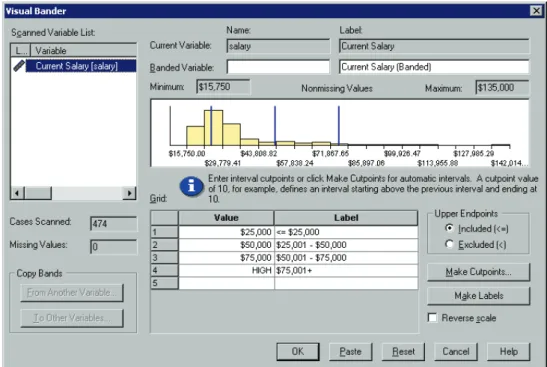
Banding Data. . . 345
Numeric Functions . . . 347
Random Number Functions . . . 348
String Concatenation . . . 349
String Parsing . . . 350
Extracting Date and Time Information . . . 353
Custom Functions, Job Flow Control, and Global Macro Variables. . . 354
Creating Custom Functions . . . 355
Job Flow Control . . . 356
Creating Global Macro Variables . . . 358
Setting Global Macro Variables to Values from the Environment. . . 359
Appendix
A Python Functions
361
spss.CreateXPathDictionary Function . . . 362 spss.Cursor Function . . . 362 spss.Cursor Methods. . . 364 spss.DeleteXPathHandle Function . . . 367 spss.EvaluateXPath Function . . . 367 spss.GetCaseCount Function . . . 368 spss.GetHandleList Function . . . 368spss.GetLastErrorLevel and spss.GetLastErrorMessage Functions . . . 369
spss.GetVariableCount Function . . . 370 spss.GetVariableFormat Function . . . 370 spss.GetVariableLabel Function . . . 373 spss.GetVariableMeasurementLevel Function. . . 373 spss.GetVariableName Function . . . 374 spss.GetVariableType Function . . . 374 spss.GetXmlUtf16 Function . . . 375 xiv
spss.SetOutput Function . . . 377 spss.StopSPSS Function . . . 377 spss.Submit Function . . . 378
Index
381
1
Overview
This book is divided into two main sections:
Data management using the SPSS command language.Although many of these tasks can also be performed with the menus and dialog boxes, some very powerful features are available only with command syntax.
Programming with SPSS and Python.The SPSS Python plug-in provides the ability to integrate the capabilities of the Python programming language with SPSS. One of the major benefits of Python is the ability to addjobwiseflow control to the SPSS command stream. SPSS can executecasewiseconditional actions based on criteria that evaluate each case, but jobwise flow control—such as running different procedures for different variables based on data type or level of measurement, or determining which procedure to run next based on the results of the last procedure—is much more difficult. The SPSS Python plug-in makes jobwise flow control much easier to accomplish.
For readers who may be more familiar with the commands in the SAS system, Chapter 19 provides examples that demonstrate how some common data management and programming tasks are handled in both SAS and SPSS.
Using This Book
This book is intended for use with SPSS release 14.0.1 or later. Many examples will work with earlier versions, but some commands and features are not available in earlier releases. None of the Python examples will work with earlier versions.
Most of the examples shown in this book are designed as hands-on exercises that you can perform yourself. The CD that comes with the book contains the command files and data files used in the examples. All of the sample files are contained in the
examplesfolder.
\examples\commandscontains SPSS command syntax files.
\examples\datacontains data files in a variety of formats.
\examples\pythoncontains sample Python files.
All of the sample command files that contain file access commands assume that you have copied the examples folder to yourCdrive. For example:
GET FILE='c:\examples\data\duplicates.sav'.
SORT CASES BY ID_house(A) ID_person(A) int_date(A) . AGGREGATE OUTFILE = 'C:\temp\tempdata.sav'
Many examples, such as the one above, also assume that you have aC:\tempfolder for writing temporary files. You can access command and data files from the accompanying CD, substituting the drive location forC:in file access commands. For commands that write files, however, you need to specify a valid folder location on a device for which you have write access.
Documentation Resources
TheSPSS Base User’s Guidedocuments the data management tools available through the graphical user interface. The material is similar to that available in the Help system.
TheSPSS Command Syntax Reference, which is installed as a PDF file with the SPSS system, is a complete guide to the specifications for each SPSS command. The guide provides many examples illustrating individual commands. It has only a few extended examples illustrating how commands can be combined to accomplish the kinds of tasks that analysts frequently encounter. Sections of theSPSS Command Syntax Referenceof particular interest include:
The appendix “Defining Complex Files,” which covers the commands specifically intended for reading common types of complex files
TheINPUT PROGRAM—END INPUT PROGRAMcommand, which provides rules for working with input programs
All of the command syntax documentation is also available in the Help system. If you type a command name or place the cursor inside a command in a syntax window and press F1, you will be taken directly to the help for that command.
2
Best Practices and Efficiency Tips
If you haven’t worked with SPSS command syntax before, you will probably start with simple jobs that perform a few basic tasks. Since it is easier to develop good habits while working with small jobs than to try to change bad habits once you move to more complex situations, you may find the information in this chapter helpful.
Some of the practices suggested in this chapter are particularly useful for large projects involving thousands of lines of code, many data files, and production jobs run on a regular basis and/or on multiple data sources.
Working with Command Syntax
You don’t need to be a programmer to write SPSS command syntax, but there are a few basic things you should know. A detailed introduction to SPSS command syntax is available in the “Universals” section in theSPSS Command Syntax Reference.
Creating Command Syntax Files
An SPSS command file is a simple text file. You can use any text editor to create a command syntax file, but SPSS provides a number of tools to make your job easier. Most features available in the graphical user interface have command syntax equivalents, and there are several ways to reveal this underlying command syntax:
Use the Paste button.Make selections from the menus and dialog boxes, and then click thePastebutton instead of theOKbutton. This will paste the underlying commands into a command syntax window.
Record commands in the log.SelectDisplay commands in the logon the Viewer tab in the Options dialog box (Edit menu, Options) or run the commandSET PRINTBACK ON. As you run analyses, the commands for your dialog box selections will be recorded and displayed in the log in the Viewer window. You can
then copy and paste the commands from the Viewer into a syntax window or text editor. This setting persists across sessions, so you have to specify it only once.
Retrieve commands from the journal file.Most actions that you perform in the graphical user interface (and all commands that you run from a command syntax window) are automatically recorded in the journal file in the form of command syntax. The default name of the journal file isspss.jnl. The default location varies, depending on your operating system. Both the name and location of the journal file are displayed on the General tab in the Options dialog box (Edit menu, Options).
Running SPSS Commands
Once you have a set of commands, you can run the commands in a number of ways:
Highlight the commands that you want to run in a command syntax window and click the Run button.
Invoke one command file from another with theINCLUDEorINSERTcommand. For more information, see “Using INSERT with a Master Command Syntax File” on p. 20.
Use the Production Facility to create production jobs that can run unattended and even start unattended (and automatically) using common scheduling software. See the Help system for more information about the Production Facility.
Use SPSSB (available only with the server version) to run command files from a command line and automatically route results to different output destinations in different formats. See the SPSSB documentation supplied with the SPSS server software for more information.
Figure 2-1
Command syntax pasted from a dialog box
Syntax Rules
Commands run from a command syntax window during a typical SPSS session must follow theinteractivecommand syntax rules.
Commands files run via SPSSB or invoked via theINCLUDEcommand must follow thebatchcommand syntax rules.
Interactive Rules
The following rules apply to command specifications in interactive mode:
Each command must start on a new line. Commands can begin in any column of a command line and continue for as many lines as needed. The exception is theEND DATAcommand, which must begin in the first column of the first line after the end of data.
Each command should end with a period as a command terminator. It is best to omit the terminator onBEGIN DATA, however, so that inline data is treated as one continuous specification.
The command terminator must be the last non-blank character in a command.
In the absence of a period as the command terminator, a blank line is interpreted as a command terminator.
Note: For compatibility with other modes of command execution (including command files run withINSERTorINCLUDEcommands in an interactive session), each line of command syntax should not exceed 256 bytes.
Batch Rules
The following rules apply to command specifications in batch or production mode:
All commands in the command file must begin in column 1. You can use plus (+) or minus (–) signs in the first column if you want to indent the command specification to make the command file more readable.
If multiple lines are used for a command, column 1 of each continuation line must be blank.
Command terminators are optional.
A line cannot exceed 256 bytes; any additional characters are truncated.
Customizing the Programming Environment
There are a few global settings and customization features that may make working with command syntax a little easier.
Displaying Commands in the Log
By default, commands that have been run are not displayed in the log, which can make it difficult to interpret error messages. To display commands in the log, use the command:
SET PRINTBACK = ON.
Or, using the graphical user interface:
E From the menus, choose:
Edit Options...
E Click theViewertab.
Figure 2-2
Log with and without commands displayed
Displaying the Status Bar in Command Syntax Windows
In addition to various status messages, the status bar at the bottom of a command syntax window displays the current line number and character position within the line. Since error messages typically contain information about the column position where an error was encountered, the column position information in the status bar can help you to pinpoint errors. (Note: You may have to increase the width of the command syntax window to see this information.)
The status bar is displayed by default. If it is currently not displayed, chooseStatus Barfrom the View menu in the command syntax window.
Figure 2-3
Status bar in command syntax window with current line number and column position displayed
Protecting the Original Data
The original data file should be protected from modifications that may alter or delete original variables and/or cases. If the original data are in an external file format (for example, text, Excel, or database), there is little risk of accidentally overwriting the original data while working in SPSS. However, if the original data are in SPSS-format data files (.sav), there are many transformation commands that can modify or destroy the data, and it is not difficult to inadvertently overwrite the contents of an SPSS-format data file. Overwriting the original data file may result in a loss of data that cannot be retrieved.
There are several ways in which you can protect the original data, including:
Storing a copy in a separate location, such as on a CD, that can’t be overwritten.
Using the operating system facilities to change the read-write property of the file to read-only. If you aren’t familiar with how to do this in the operating system, you can chooseMark File Read Onlyfrom the File menu or use thePERMISSIONS
subcommand on theSAVEcommand.
The ideal situation is then to load the original (protected) data file into SPSS and do
alldata transformations, recoding, and calculations using SPSS. The objective is to end up with one or more command syntax files that start from the original data and produce the required results without any manual intervention.
Do Not Overwrite Original Variables
It is often necessary to recode or modify original variables, and it is good practice to assign the modified values to new variables and keep the original variables unchanged. For one thing, this allows comparison of the initial and modified values to verify that the intended modifications were carried out correctly. The original values can subsequently be discarded if required.
Example
*These commands overwrite existing variables. COMPUTE var1=var1*2.
RECODE var2 (1 thru 5 = 1) (6 thru 10 = 2). *These commands create new variables. COMPUTE var1_new=var1*2.
RECODE var2 (1 thru 5 = 1) (6 thru 10 = 2)(ELSE=COPY) /INTO var2_new.
The difference between the twoCOMPUTEcommands is simply the substitution of a new variable name on the left side of the equals sign.
The secondRECODEcommand includes theINTOsubcommand, which specifies a new variable to receive the recoded values of the original variable.ELSE=COPY
makes sure that any values not covered by the specified ranges are preserved.
Using Temporary Transformations
You can use theTEMPORARYcommand to temporarily transform existing variables for analysis. The temporary transformations remain in effect through the first command that reads the data (for example, a statistical procedure), after which the variables revert to their original values.
Example
*temporary.sps.
DATA LIST FREE /var1 var2. BEGIN DATA 1 2 3 4 5 6 7 8 9 10 END DATA. TEMPORARY.
COMPUTE var1=var1+ 5.
RECODE var2 (1 thru 5=1) (6 thru 10=2). FREQUENCIES
/VARIABLES=var1 var2
/STATISTICS=MEAN STDDEV MIN MAX. DESCRIPTIVES
/VARIABLES=var1 var2
/STATISTICS=MEAN STDDEV MIN MAX.
The transformed values from the two transformation commands that follow the
TEMPORARYcommand will be used in theFREQUENCIESprocedure.
The original data values will be used in the subsequentDESCRIPTIVESprocedure, yielding different results for the same summary statistics.
Under some circumstances, usingTEMPORARYwill improve the efficiency of a job when short-lived transformations are appropriate. Ordinarily, the results of transformations are written to the virtual active file for later use and eventually are merged into the saved SPSS data file. However, temporary transformations will not be written to disk, assuming that the command that concludes the temporary state is not otherwise doing this, saving both time and disk space. (TEMPORARYfollowed by
SAVE, for example, would write the transformations.)
If many temporary variables are created, not writing them to disk could be a noticeable saving with a large data file. However, some commands require two or more passes of the data. In this situation, the temporary transformations are recalculated for the second or later passes. If the transformations are lengthy and complex, the time required for repeated calculation might be greater than the time saved by not writing the results to disk. Experimentation may be required to determine which approach is more efficient.
Using Temporary Variables
For transformations that require intermediate variables, use scratch (temporary) variables for the intermediate values. Any variable name that begins with a pound sign (#) is treated as a scratch variable that is discarded at the end of the series of transformation commands when SPSS encounters anEXECUTEcommand or other command that reads the data (such as a statistical procedure).
Example
*scratchvar.sps. DATA LIST FREE / var1. BEGIN DATA
1 2 3 4 5 END DATA.
COMPUTE factor=1.
LOOP #tempvar=1 TO var1.
- COMPUTE factor=factor * #tempvar. END LOOP.
EXECUTE.
Figure 2-4
Result of loop with scratch variable
The loop structure computes the factorial for each value ofvar1and puts the factorial value in the variablefactor.
The scratch variable#tempvaris used as an index variable for the loop structure.
For each case, theCOMPUTEcommand is run iteratively up to the value ofvar1.
For each iteration, the current value of the variablefactoris multiplied by the current loop iteration number stored in#tempvar.
TheEXECUTEcommand runs the transformation commands, after which the scratch variable is discarded.
The use of scratch variables doesn’t technically “protect” the original data in any way, but it does prevent the data file from getting cluttered with extraneous variables. If you need to remove temporary variables that still exist after reading the data, you can use theDELETE VARIABLEScommand to eliminate them.
Use EXECUTE Sparingly
SPSS is designed to work with large data files (the current version can accommodate 2.15 billion cases). Since going through every case of a large data file takes time, the software is also designed to minimize the number of times it has to read the data. Statistical and charting procedures always read the data, but most transformation commands (for example,COMPUTE,RECODE,COUNT,SELECT IF) do not require a separate data pass.
The default behavior of the graphical user interface, however, is to read the data for each separate transformation so that you can see the results in the Data Editor immediately. Consequently, every transformation command generated from the dialog boxes is followed by anEXECUTEcommand. So if you create command syntax by pasting from dialog boxes or copying from the log or journal, your command syntax may contain a large number of superfluousEXECUTEcommands that can significantly increase the processing time for very large data files.
In most cases, you can remove virtually all of the auto-generatedEXECUTE
commands, which will speed up processing, particularly for large data files and jobs that contain many transformation commands.
To turn off the automatic, immediate execution of transformations and the associated pasting ofEXECUTEcommands:
E From the menus, choose:
Edit Options...
E Click theDatatab.
E SelectCalculate values before used.
Lag Functions
One notable exception to the above rule is transformation commands that contain lag functions. In a series of transformation commands without any interveningEXECUTE
commands or other commands that read the data, lag functions are calculated after all other transformations, regardless of command order. While this might not be a consideration most of the time, it requires special consideration in the following cases:
One of the transformations selects a subset of cases and deletes the unselected cases, such asSELECT IF or SAMPLE.
Example
*lagfunction.sps. *create some data. DATA LIST FREE /var1. BEGIN DATA
1 2 3 4 5 END DATA.
COMPUTE var2=var1.
********************************. *Lag without intervening EXECUTE. COMPUTE lagvar1=LAG(var1).
COMPUTE var1=var1*2. EXECUTE.
********************************. *Lag with intervening EXECUTE. COMPUTE lagvar2=LAG(var2). EXECUTE.
COMPUTE var2=var2*2. EXECUTE.
Figure 2-5
Results of lag functions displayed in Data Editor
Althoughvar1andvar2contain the same data values,lagvar1andlagvar2are very different from each other.
Without an interveningEXECUTEcommand,lagvar1is based on the transformed values ofvar1.
With theEXECUTEcommand between the two transformation commands, the value oflagvar2is based on the original value ofvar2.
Any command that reads the data will have the same effect as theEXECUTE
command. For example, you could substitute theFREQUENCIEScommand and achieve the same result.
In a similar fashion, if the set of transformations includes a command that selects a subset of cases and deletes unselected cases (for example,SELECT IF), lags will be computed after the case selection. You will probably want to avoid case selection criteria based on lag values—unless youEXECUTEthe lags first.
Using $CASENUM to Select Cases
The value of the system variable$CASENUMis dynamic. If you change the sort order of cases, the value of$CASENUMfor each case changes. If you delete the first case, the case that formerly had a value of 2 for this system variable now has the value 1. Using the value of$CASENUMwith the SELECT IF command can be a little tricky becauseSELECT IFdeletes each unselected case, changing the value of$CASENUM
for all remaining cases.
For example, aSELECT IFcommand of the general form: SELECT IF ($CASENUM > [positive value]).
will delete all cases because, regardless of the value specified, the value of$CASENUM
for the current case will never be greater than 1. When the first case is evaluated, it has a value of 1 for$CASENUMand is therefore deleted because it doesn’t have a value greater than the specified positive value. The erstwhile second case then becomes the first case, with a value of 1, and is consequently also deleted, and so on.
The simple solution to this problem is to create a new variable equal to the original value of$CASENUM. However, command syntax of the form:
COMPUTE CaseNumber=$CASENUM.
SELECT IF (CaseNumber > [positive value]).
will still delete all cases because each case is deleted before the value of the new variable is computed. The correct solution is to insert anEXECUTEcommand between
COMPUTEandSELECT IF, as in: COMPUTE CaseNumber=$CASENUM.
EXECUTE.
SELECT IF (CaseNumber > [positive value]).
MISSING VALUES Command
If you have a series of transformation commands (for example,COMPUTE,IF,RECODE) followed by aMISSING VALUEScommand that involves the same variables, you may want to place anEXECUTEstatement before theMISSING VALUEScommand. This is because theMISSING VALUEScommand changes the dictionary before the transformations take place.
Example
IF (x = 0) y = z*2. MISSING VALUES x (0).
The cases wherex = 0would be considered user-missing onx, and the transformation ofywould not occur. Placing anEXECUTEbeforeMISSING VALUESallows the transformation to occur before 0 is assigned missing status.
WRITE and XSAVE Commands
In some circumstances, it may be necessary to have anEXECUTEcommand after a
WRITEor anXSAVEcommand. For more information, see “Using XSAVE in a Loop to Build a Data File” in Chapter 8 on p. 156.
Using Comments
It is always a good practice to include explanatory comments in your code. In SPSS, you can do this in several ways:
COMMENT Get summary stats for scale variables.
* An asterisk in the first column also identifies comments. FREQUENCIES
VARIABLES=income ed reside
/FORMAT=LIMIT(10) /*avoid long frequency tables /STATISTICS=MEAN /*arithmetic average*/ MEDIAN.
* A macro name like !mymacro in this comment may invoke the macro.
The first line of a comment can begin with the keywordCOMMENTor with an asterisk (*).
Comment text can extend for multiple lines and can contain any characters. The rules for continuation lines are the same as for other commands. Be sure to terminate a comment with a period.
Use /* and */ to set off a comment within a command.
The closing */ is optional when the comment is at the end of the line. The command can continue onto the next line just as if the inserted comment were a blank.
To ensure that comments that refer to macros by name don’t accidently invoke those macros, use the/* [comment text] */format.
Using SET SEED to Reproduce Random Samples or Values
When doing research involving random numbers—for example, when randomly assigning cases to experimental treatment groups—you should explicitly set the random number seed value if you want to be able to reproduce the same results.
The random number generator is used by theSAMPLEcommand to generate random samples and is used by many distribution functions (for example,NORMAL,UNIFORM) to generate distributions of random numbers. The generator begins with aseed, a large integer. Starting with the same seed, the system will repeatedly produce the same sequence of numbers and will select the same sample from a given data file. At the start of each session, the seed is set to a value that may vary or may be fixed, depending on your current settings. The seed value changes each time a series of transformations contains one or more commands that use the random number generator.
Example
To repeat the same random distribution within a session or in subsequent sessions, use
SET SEEDbefore each series of transformations that use the random number generator to explicitly set the seed value to a constant value.
*set_seed.sps.
GET FILE = 'c:\examples\data\onevar.sav'. SET SEED = 123456789.
SAMPLE .1. LIST.
GET FILE = 'c:\examples\data\onevar.sav'. SET SEED = 123456789.
SAMPLE .1. LIST.
Before the first sample is taken the first time, the seed value is explicitly set with
SET SEED.
TheLISTcommand causes the data to be read and the random number generator to be invoked once for each original case. The result is an updated seed value.
The second time the data file is opened,SET SEEDsets the seed to the same value as before, resulting in the same sample of cases.
BothSET SEEDcommands are required because you aren’t likely to know what the initial seed value is unless you set it yourself.
Note: This example opens the data file before eachSAMPLEcommand because successiveSAMPLEcommands arecumulativewithin the active dataset.
SET SEED versus SET MTINDEX
SPSS provides two random number generators, andSET SEEDsets the starting value for only the default random number generator (SET RNG=MC). If you are using the newer Mersenne Twister random number generator (SET RNG=MT), the starting value is set withSET MTINDEX.
Divide and Conquer
A time-proven method of winning the battle against programming bugs is to split the tasks into separate, manageable pieces. It is also easier to navigate around a syntax file of 200–300 lines than one of 2,000–3,000 lines.
Therefore, it is good practice to break down a program into separate stand-alone files, each performing a specific task or set of tasks. For example, you could create separate command syntax files to:
Prepare and standardize data.
Merge data files.
Perform tests on data.
Report results for different groups (for example, gender, age group, income category).
Using theINSERTcommand and a master command syntax file that specifies all of the other command files, you can partition all of these tasks into separate command files.
Using INSERT with a Master Command Syntax File
TheINSERTcommand provides a method for linking multiple syntax files together, making it possible to reuse blocks of command syntax in different projects by using a “master” command syntax file that consists primarily ofINSERTcommands that refer to other command syntax files.
Example
INSERT FILE = "c:\examples\data\prepare data.sps" CD=YES. INSERT FILE = "combine data.sps".
INSERT FILE = "do tests.sps". INSERT FILE = "report groups.sps".
EachINSERTcommand specifies a file that contains SPSS command syntax.
By default, inserted files are read usinginteractivesyntax rules, and each command should end with a period.
The firstINSERTcommand includes the additional specificationCD=YES. This changes the working directory to the directory included in the file specification, making it possible to use relative (or no) paths on the subsequentINSERT
commands.
INSERT versus INCLUDE
INSERTis a newer, more powerful and flexible alternative toINCLUDE. Files included withINCLUDEmust always adhere to batch syntax rules, and command processing stops when the first error in an included file is encountered. You can effectively duplicate theINCLUDEbehavior withSYNTAX=BATCHandERROR=STOPon the
INSERTcommand.
Defining Global Settings
In addition to usingINSERTto create modular master command syntax files, you can define global settings that will enable you to use those same command files for different reports and analyses.
Example
You can create a separate command syntax file that contains a set ofFILE HANDLE
commands that define file locations and a set of macros that define global variables for client name, output language, and so on. When you need to change any settings, you change them once in the global definition file, leaving the bulk of the command syntax files unchanged.
*define_globals.sps.
FILE HANDLE data /NAME='c:\examples\data'.
FILE HANDLE commands /NAME='c:\examples\commands'. FILE HANDLE spssdir /NAME='c:\program files\spss'. FILE HANDLE tempdir /NAME='d:\temp'.
DEFINE !enddate()DATE.DMY(1,1,2004)!ENDDEFINE. DEFINE !olang()English!ENDDEFINE.
DEFINE !client()"ABC Inc"!ENDDEFINE. DEFINE !title()TITLE !client.!ENDDEFINE.
The first twoFILE HANDLEcommands define the paths for the data and command syntax files. You can then use these file handles instead of the full paths in any file specifications.
The thirdFILE HANDLEcommand contains the path to the SPSS folder. This path can be useful if you use any of the command syntax or script files that are installed with SPSS.
The lastFILE HANDLEcommand contains the path of a temporary folder. It is very useful to define a temporary folder path and use it to save any intermediary files created by the various command syntax files making up the project. The main purpose of this is to avoid crowding the data folders with useless files, some of which might be very large. Note that here the temporary folder resides on theD
drive. When possible, it is more efficient to keep the temporary and main folders on different hard drives.
TheDEFINE–!ENDDEFINEstructures define a series of macros. This example uses simple string substitution macros, where the defined strings will be substituted wherever the macro names appear in subsequent commands during the session.
!enddatecontains the end date of the period covered by the data file. This can be useful to calculate ages or other duration variables as well as to add footnotes to tables or graphs.
!clientcontains the client’s name. This can be used in titles of tables or graphs.
!titlespecifies aTITLEcommand, using the value of the macro!clientas the title text.
The master command syntax file might then look something like this: INSERT FILE = "c:\examples\commands\define_globals.sps". !title.
INSERT FILE = "data\prepare data.sps". INSERT FILE = "commands\combine data.sps". INSERT FILE = "commands\do tests.sps". INCLUDE FILE = "commands\report groups.sps".
The firstINSERTruns the command syntax file that defines all of the global settings. This needs to be run before any commands that invoke the macros defined in that file.
!titlewill print the client’s name at the top of each page of output.
"data"and"commands"in the remainingINSERTcommands will be expanded to"c:\examples\data"and"c:\examples\commands", respectively.
Note: Using absolute paths or file handles that represent those paths is the most reliable way to make sure that SPSS finds the necessary files. Relative paths may not work as you might expect, since they refer to the current working directory, which can change frequently. You can also use theCDcommand or theCDkeyword on theINSERT
3
Getting Data into SPSS
Before you can work with data in SPSS, you need some data to work with. There are several ways to get data into the application:
Open a data file that has already been saved in SPSS format.
Enter data manually in the Data Editor.
Read a data file from another source, such as a database, text data file, spreadsheet, SAS, or Stata.
Opening an SPSS-format data file is simple, and manually entering data in the Data Editor is not likely to be your first choice, particularly if you have a large amount of data. This chapter focuses on how to read data files created and saved in other applications and formats.
Getting Data from Databases
SPSS relies primarily on ODBC (open database connectivity) to read data from databases. ODBC is an open standard with versions available on many platforms, including Windows, UNIX, and Macintosh.
Installing Database Drivers
You can read data from any database format for which you have a database driver. In local analysis mode, the necessary drivers must be installed on your local computer. In distributed analysis mode (available with the Server version), the drivers must be installed on the remote server.
ODBC database drivers for a wide variety of database formats are included on the SPSS installation CD, including:
Access
Btrieve DB2 dBASE Excel FoxPro Informix Oracle Paradox Progress SQL Base SQL Server Sybase
Most of these drivers can be installed by installing the SPSS Data Access Pack. You can install the SPSS Data Access Pack from the AutoPlay menu on the SPSS installation CD.
If you need a Microsoft Access driver, you will need to install the Microsoft Data Access Pack. An installable version is located in theMicrosoft Data Access Pack
folder on the SPSS installation CD.
Before you can use the installed database drivers, you may also need to configure the drivers using the Windows ODBC Data Source Administrator. For the SPSS Data Access Pack, installation instructions and information on configuring data sources are located in theInstallation Instructionsfolder on the SPSS installation CD.
OLE DB
Starting with SPSS 14.0, some support for OLE DB data sources is provided. To access OLE DB data sources, you must have the following items installed on the computer that is running SPSS:
.NET framework
Dimensions Data Model and OLE DB Access
Versions of these components that are compatible with this release of SPSS can be installed from the SPSS installation CD and are available on the AutoPlay menu.
Table joins are not available for OLE DB data sources. You can read only one table at a time.
You can add OLE DB data sources only in local analysis mode. To add OLE DB data sources in distributed analysis mode on a Windows server, consult your system administrator.
In distributed analysis mode (available with SPSS Server), OLE DB data sources are available only on Windows servers, and both .NET and the Dimensions Data Model and OLE DB Access must be installed on the server.
Database Wizard
It’s probably a good idea to use the Database Wizard (File menu, Open Database) the first time you retrieve data from a database source. At the last step of the wizard, you can paste the equivalent commands into a command syntax window. Although the SQL generated by the wizard tends to be overly verbose, it also generates theCONNECT
string, which you might never figure out without the wizard.
Reading a Single Database Table
SPSS reads data from databases by reading database tables. You can read information from a single table or merge data from multiple tables in the same database. A single database table has basically the same two-dimensional structure as an SPSS data file: records are cases and fields are variables. So, reading a single table can be very simple.
Example
This example reads a single table from an Access database. It reads all records and fields in the table.
*access1.sps.
GET DATA /TYPE=ODBC /CONNECT=
'DSN=MS Access Database;DBQ=C:\examples\data\dm_demo.mdb;'+ 'DriverId=25;FIL=MS Access;MaxBufferSize=2048;PageTimeout=5;' /SQL = 'SELECT * FROM CombinedTable'.
EXECUTE.
TYPE=ODBCindicates that an ODBC driver will be used to read the data. This is required for reading data from any database, and it can also be used for other data sources with ODBC drivers, such as Excel workbooks. For more information, see “Reading Multiple Worksheets” on p. 33.
CONNECTidentifies the data source. For this example, theCONNECTstring was copied from the command syntax generated by the Database Wizard. The entire string must be enclosed in single or double quotes. In this example, we have split the long string onto two lines using a plus sign (+) to combine the two strings.
TheSQLsubcommand can contain any SQL statements supported by the database format. Each line must be enclosed in single or double quotes.
SELECT * FROM CombinedTablereads all of the fields (columns) and all records (rows) from the table namedCombinedTablein the database.
Any field names that are not valid SPSS variable names are automatically converted to valid variable names, and the original field names are used as variable labels. In this database table, many of the field names contain spaces, which are removed in the variable names.
Figure 3-1
Database field names converted to valid variable names
Example
Now we’ll read the same database table—except this time, we’ll read only a subset of fields and records.
*access2.sps.
GET DATA /TYPE=ODBC /CONNECT=
'DSN=MS Access Database;DBQ=C:\examples\data\dm_demo.mdb;'+ 'DriverId=25;FIL=MS Access;MaxBufferSize=2048;PageTimeout=5;' /SQL =
'SELECT Age, Education, [Income Category]' ' FROM CombinedTable'
' WHERE ([Marital Status] <> 1 AND Internet = 1 )'. EXECUTE.
TheSELECTclause explicitly specifies only three fields from the file; so, the active dataset will contain only three variables.
TheWHEREclause will select only records where the value of theMarital Status
field is not 1 and the value of theInternetfield is 1. In this example, that means only unmarried people who have Internet service will be included.
Two additional details in this example are worth noting:
The field namesIncome CategoryandMarital Statusare enclosed in brackets. Since these field names contain spaces, they must be enclosed in brackets or quotes. Since single quotes are already being used to enclose each line of the SQL statement, the alternative to brackets here would be double quotes.
We’ve put theFROMandWHEREclauses on separate lines to make the code easier to read; however, in order for this command to be read properly, each of those lines also has a blank space between the starting single quote and the first word on the line. When the command is processed, all of the lines of the SQL statement are merged together in a very literal fashion. Without the space beforeWHERE, the program would attempt to read a table namedCombinedTableWhere, and an error would result. As a general rule, you should probably insert a blank space between the quotation mark and the first word of each continuation line.
Reading Multiple Tables
You can combine data from two or more database tables by “joining” the tables. The active dataset can be constructed from more than two tables, but each “join” defines a relationship between only two of those tables:
Inner join.Records in the two tables with matching values for one or more specified fields are included. For example, a unique ID value may be used in each table, and records with matching ID values are combined. Any records without matching identifier values in the other table are omitted.
Left outer join.All records from the first table are included regardless of the criteria used to match records.
Right outer join.Essentially the opposite of a left outer join. So, the appropriate one to use is basically a matter of the order in which the tables are specified in the SQLSELECTclause.
Example
In the previous two examples, all of the data resided in a single database table. But what if the data were divided between two tables? This example merges data from two different tables: one containing demographic information for survey respondents and one containing survey responses.
*access_multtables1.sps. GET DATA /TYPE=ODBC /CONNECT=
'DSN=MS Access Database;DBQ=C:\examples\data\dm_demo.mdb;'+ 'DriverId=25;FIL=MS Access;MaxBufferSize=2048;PageTimeout=5;' /SQL =
'SELECT * FROM DemographicInformation, SurveyResponses' ' WHERE DemographicInformation.ID=SurveyResponses.ID'. EXECUTE.
TheSELECTclause specifies all fields from both tables.
TheWHEREclause matches records from the two tables based on the value of the
IDfield in both tables. Any records in either table without matchingIDvalues in the other table are excluded.
The result is an inner join in which only records with matchingIDvalues in both tables are included in the active dataset.
Example
In addition to one-to-one matching, as in the previous inner join example, you can also merge tables with a one-to-many matching scheme. For example, you could match a table in which there are only a few records representing data values and associated descriptive labels with values in a table containing hundreds or thousands of records representing survey respondents.
In this example, we read data from an SQL Server database, using an outer join to avoid omitting records in the larger table that don’t have matching identifier values in the smaller table.
*sqlserver_outer_join.sps. GET DATA /TYPE=ODBC
/CONNECT= 'DSN=SQLServer;UID=;APP=SPSS For Windows;' 'WSID=ROLIVERLAP;Network=DBMSSOCN;Trusted_Connection=Yes' /SQL =
'SELECT SurveyResponses.ID, SurveyResponses.Internet,' ' [Value Labels].[Internet Label]'
' FROM SurveyResponses LEFT OUTER JOIN [Value Labels]' ' ON SurveyResponses.Internet'
' = [Value Labels].[Internet Value]'.
Figure 3-2
Figure 3-3
Active dataset in SPSS
FROM SurveyResponses LEFT OUTER JOIN [Value Labels]will include all records from the tableSurveyResponseseven if there are no records in theValue Labelstable that meet the matching criteria.
ON SurveyResponses.Internet = [Value Labels].[Internet Value]matches records based on the value of the fieldInternetin the table
SurveyResponsesand the value of the fieldInternet Valuein the tableValue Labels.
The resulting active dataset has anInternet Labelvalue ofNofor all cases with a value of 0 forInternetandYesfor all cases with a value of 1 forInternet.
Since the left outer join includes all records fromSurveyResponses, there are cases in the active dataset with values of 8 or 9 forInternetand no value (a blank string) forInternet Label, since the values of 8 and 9 do not occur in theInternet Value
field in the tableValue Labels.
Reading Excel Files
SPSS can read individual Excel worksheets and multiple worksheets in the same Excel workbook. The basic mechanics of reading Excel files are relatively
straightforward—rows are read as cases and columns are read as variables. However, reading a typical Excel spreadsheet—where the data may not start in row 1,
column 1—requires a little extra work, and reading multiple worksheets requires treating the Excel workbook as a database. In both instances, we can use theGET DATAcommand to read the data into SPSS.
Reading a “Typical” Worksheet
When reading an individual worksheet, SPSS reads a rectangular area of the worksheet, and everything in that area must be data related. The first row of the area may or may not contain variable names (depending on your specifications); the remainder of the area must contain the data to be read. A typical worksheet, however, may also contain titles and other information that may not be appropriate for an SPSS data file and may even cause the data to be read incorrectly if you don’t explicitly specify the range of cells to read.
Example Figure 3-4
To read this spreadsheet without the title row or total row and column: *readexcel.sps.
GET DATA /TYPE=XLS
/FILE='c:\examples\data\sales.xls' /SHEET=NAME 'Gross Revenue'
/CELLRANGE=RANGE 'A2:I15' /READNAMES=on .
TheTYPEsubcommand identifies the file type as Excel, version 5 or later. (For earlier versions, useGET TRANSLATE.)
TheSHEETsubcommand identifies which worksheet of the workbook to read. Instead of theNAMEkeyword, you could use theINDEXkeyword and an integer value indicating the sheet location in the workbook. Without this subcommand, the first worksheet is read.
TheCELLRANGEsubcommand indicates that SPSS should start reading at column
A, row 2, and read through columnI, row 15.
TheREADNAMESsubcommand indicates that the first row of the specified range contains column labels to be used as variable names.
Figure 3-5
The Excel column labelStore Numberis automatically converted to the SPSS variable nameStoreNumber, since variable names cannot contain spaces. The original column label is retained as the variable label.
The original data type from Excel is preserved whenever possible, but since data type is determined at the individual cell level in Excel and at the column (variable) level in SPSS, this isn’t always possible.
When SPSS encounters mixed data types in the same column, the variable is assigned the string data type; so, the variableToysin this example is assigned the string data type.
READNAMES Subcommand
TheREADNAMESsubcommand tells SPSS to treat the first row of the spreadsheet or specified range as either variable names (ON) or data (OFF). This subcommand will always affect the way the Excel spreadsheet is read, even when it isn’t specified, since the default setting isON.
WithREADNAMES=ON(or in the absence of this subcommand), if the first row contains data instead of column headings, SPSS will attempt to read the cells in that row as variable names instead of as data—alphanumeric values will be used to create variable names, numeric values will be ignored, and default variable names will be assigned.
WithREADNAMES=OFF, if the first row does, in fact, contain column headings or other alphanumeric text, then those column headings will be read as data values, and all of the variables will be assigned the string data type.
Reading Multiple Worksheets
An Excel file (workbook) can contain multiple worksheets, and you can read multiple worksheets from the same workbook by treating the Excel file as a database. This requires an ODBC driver for Excel.
Figure 3-6
Multiple worksheets in same workbook
When reading multiple worksheets, you lose some of the flexibility available for reading individual worksheets:
You cannot specify cell ranges.
The first non-empty row of each worksheet should contain column labels that will be used as variable names.
Only basic data types—string and numeric—are preserved, and string variables may be set to an arbitrarily long width.
Example
In this example, the first worksheet contains information about store location, and the second and third contain information for different departments. All three contain a column,Store Number, that uniquely identifies each store, so, the information in the three sheets can be merged correctly regardless of the order in which the stores are listed on each worksheet.
*readexcel2.sps. GET DATA /TYPE=ODBC /CONNECT= 'DSN=Excel Files;DBQ=c:\examples\data\sales.xls;' + 'DriverId=790;MaxBufferSize=2048;PageTimeout=5;' /SQL =
'SELECT Location$.[Store Number], State, Region, City,' ' Power, Hand, Accessories,'
' Tires, Batteries, Gizmos, Dohickeys' ' FROM [Location$], [Tools$], [Auto$]'
' WHERE [Tools$].[Store Number]=[Location$].[Store Number]' ' AND [Auto$].[Store Number]=[Location$].[Store Number]'.
If these commands look like random characters scattered on the page to you, try using the Database Wizard (File menu, Open Database) and, in the last step, paste the commands into a syntax window.
Even if you are familiar with SQL statements, you may want to use the Database Wizard the first time to generate the properCONNECTstring.
TheSELECTstatement specifies the columns to read from each worksheet, as identified by the column headings. Since all three worksheets have a column labeledStore Number, the specific worksheet from which to read this column is also included.
If the column headings can’t be used as variable names, you can either let SPSS automatically create valid variable names or use theASkeyword followed by a valid variable name. In this example,Store Numberis not a valid SPSS variable name; so, a variable name ofStoreNumberis automatically created, and the original column heading is used as the variable label.
TheFROMclause identifies the worksheets to read.
TheWHEREclause indicates that the data should be merged by matching the values of the columnStore Numberin the three worksheets.
Figure 3-7
Merged worksheets in SPSS
Reading Text Data Files
A text data file is simply a text file that contains data. Text data files fall into two broad categories:
Simpletext data files, in which all variables are recorded in the same order for all cases, and all cases contain the same variables. This is basically how all data files appear once they are read into SPSS.
Complextext data files, including files in which the order of variables may vary between cases and hierarchical or nested data files in which some records contain variables with values that apply to one or more cases contained on subsequent records that contain a different set of variables (for example, city, state, and street address on one record and name, age, and gender of each household member on subsequent records).
Text data files can be further subdivided into two more categories:
Delimited.Spaces, commas, tabs, or other characters are used to separate variables. The variables are recorded in the same order for each case but not necessarily in the same column locations. This is also referred to asfreefieldformat. Some
applications export text data in comma-separated values (CSV) format; this is a delimited format.
Fixed width.Each variable is recorded in the same column location on the same line (record) for each case in the data file. No delimiter is required between values. In fact, in many text data files generated by computer programs, data values may appear to run together without even spaces separating them. The column location determines which variable is being read.
Complex data files are typically also fixed-width format data files.
Simple Text Data Files
In most cases, the Text Wizard (File menu, Read Text Data) provides all of the functionality that you need to read simple text data files. You can preview the original text data file and resulting SPSS data file as you make your choices in the wizard, and you can paste the command syntax equivalent of your choices into a command syntax window at the last step.
Two commands are available for reading text data files: GET DATAandDATA LIST. In many cases, they provide the same functionality, and the choice of one versus the other is a matter of personal preference. In some instances, however, you may need to take advantage of features in one command that aren’t available in the other.
GET DATA
UseGET DATAinstead ofDATA LISTif:
The file is in CSV format.
The text data file is very large.
DATA LIST
UseDATA LISTinstead ofGET DATAif:
The text data is “inline” data contained in a command syntax file usingBEGIN DATA–END DATA.
The file has a complex structure, such as a mixed or hierarchical structure. For more information, see “Reading Complex Text Data Files” on p. 49.
You want to use theTOkeyword to define a large number of sequential variable names (for example,var1 TO var1000).
Many examples in other chapters useDATA LISTto define sample data simply because it supports the use of inline data contained in the command syntax file rather than in an external data file, making the examples self-contained and requiring no additional files to work.
Delimited Text Data
In a simple delimited (or “freefield”) text data file, the absolute position of each variable isn’t important; only the relative position matters. Variables should be recorded in the same order for each case, but the actual column locations aren’t relevant. More than one case can appear on the same record, and some records can span multiple records, while others do not.
Example
One of the advantages of delimited text data files is that they don’t require a great deal of structure. The sample data file,simple_delimited.txt, looks like this:
1 m 28 1 2 2 1 2 2 f 29 2 1 2 1 2 003 f 45 3 2 1 4 5 128 m 17 1 1 1 9 4
TheDATA LISTcommand to read the data file is: *simple_delimited.sps.
DATA LIST FREE
FILE = 'c:\examples\data\simple_delimited.txt'
/id (F3) sex (A1) age (F2) opinion1 TO opinion5 (5F). EXECUTE.
FREEindicates that the text data file is a delimited file, in which only the order of variables matters. By default, commas and spaces are read as delimiters between data values. In this example, all of the data values are separated by spaces.
Eight variables are defined; so, after reading eight values, the next value is read as the first variable for the next case, even if it’s on the same line. If the end of a record is reached before eight values have been read for the current case, the first value on the next line is read as the next value for the current case. In this example, four cases are contained on three records.