Michael C. Frank
Department of Psychology, Stanford University
Sharon Goldwater
School of Informatics, University of Edinburgh
Thomas L. Gri
ffi
ths
Department of Psychology, University of California, Berkeley
Joshua B. Tenenbaum
Department of Brain and Cognitive Sciences, Massachusetts Institute of Technology
The ability to discover groupings in continuous stimuli on the basis of distributional infor-mation is present across species and across perceptual modalities. We investigate the nature of the computations underlying this ability using statistical word segmentation experiments in which we vary the length of sentences, the amount of exposure, and the number of words in the languages being learned. Although the results are intuitive from the perspective of a language learner (longer sentences, less training, and a larger language all make learning more difficult), standard computational proposals fail to capture several of these results. We describe how probabilistic models of segmentation can be modified to take into account some notion of memory or resource limitations in order to provide a closer match to human performance.
Human adults and infants, non-human primates, and even rodents all show a surprising ability: presented with a stream of syllables with no pauses between them, individuals from each group are able to discriminate statistically coherent se-quences from sese-quences with lower coherence (Aslin, Saf-fran, & Newport, 1998; Hauser, Newport, & Aslin, 2001; Saffran, Johnson, Aslin, & Newport, 1999; Saffran, Newport, & Aslin, 1996; Toro & Trobalon, 2005). This ability is not unique to linguistic stimuli (Saffran et al., 1999) or to the auditory domain (Conway & Christiansen, 2005; Kirkham, Slemmer, & Johnson, 2002), and is not constrained to tempo-ral sequences (Fiser & Aslin, 2002) or even to the particulars of perceptual stimuli (Brady & Oliva, 2008). This “statistical learning” ability may be useful for a large variety of tasks but is especially relevant to language learners who must learn to segment words from fluent speech.
Yet despite the scope of the “statistical learning” phe-nomenon and the large literature surrounding it, the computa-tions underlying statistical learning are at present unknown. Following an initial suggestion by Harris (1951), work on this topic by Saffran and colleagues (Saffran, Aslin, & New-port, 1996; Saffran, Newport, & Aslin, 1996) suggested that
We gratefully acknowledge Elissa Newport and Richard Aslin for many valuable discussions of this work and thank LouAnn Gerken, Pierre Perruchet, and two anonymous reviewers for com-ments on the paper. Portions of the data in this paper were reported at the Cognitive Science conference in Frank, Goldwater, Mans-inghka, Griffiths, and Tenenbaum (2007). We acknowledge NSF grant #BCS-0631518, and the first author was supported by a Jacob Javits Graduate Fellowship and NSF DDRIG #0746251.
Please address correspondence to Michael C. Frank, Depart-ment of Psychology, Stanford University, 450 Serra Mall, Jordan Hall (Building 420), Stanford, CA 94305, tel: (650) 724-4003, email: [email protected].
learners could succeed in word segmentation by computing transitional probabilities between syllables and using low-probability transitions as one possible indicator of a bound-ary between words. More recently, a number of investi-gations have used more sophisticated computational mod-els to attempt to characterize the computations performed by human learners in word segmentation (Giroux & Rey, 2009) and visual statistical learning (Orb´an, Fiser, Aslin, & Lengyel, 2008) tasks.
The goal of the current investigation is to extend this pre-vious work by evaluating a larger set of models against new experimental data describing human performance in statis-tical word segmentation tasks. Our strategy is to investi-gate the fit of segmentation models to human performance. Because existing experiments show evidence of statistical segmentation but provide only limited quantitative results about segmentation under different conditions, we parametri-cally manipulate basic factors leading to difficulty for human learners to create a relatively detailed dataset with which to evaluate models.
The plan of the paper is as follows. We first review some previous work on the computations involved in statistical learning. Next, we make use of the adult statistical seg-mentation paradigm of Saffran, Newport, and Aslin (1996) to measure human segmentation performance as we vary three factors: sentence length, amount of exposure, and number of words in the language. We then evaluate a variety of seg-mentation models on the same dataset and find that although some of the results are well-modeled by some subset of mod-els, no model captures all three results. We argue that the likely cause of this failure is the lack of memory constraints on current models. We conclude by considering methods for modifying models of segmentation to better reflect the mem-ory constraints on human learning.
There are three contributions of this work: we intro-duce a variety of new human data about segmentation
un-der a range of experimental conditions, we show an impor-tant limitation of a number of proposed models, and we de-scribe a broad class of models—memory-limited probabilis-tic models—which we believe should be the focus of atten-tion in future investigaatten-tions.
Computations Underlying Statistical Learning
Investigations of the computations underlying statisti-cal learning phenomena have followed two complementary strategies. The first strategy is the strategy of evaluating model sufficiency: whether a particular model, given some fixed amount of data, will converge to the correct solution. If a model does not converge to the correct solution within the amount of data available to a human learner, either the model is incorrect or the human learner relies on other sources of information to solve the problem. The second strategy eval-uatesfidelity: the fit between model performance and human performance across a range of different inputs. To the extent that a model correctly matches the pattern of successes and failures exhibited by human learners, it can be said to provide a better theory of human learning.
Investigations of the sufficiency of different computational proposals for segmentation have suggested that transitional probabilities may not be a viable segmentation strategy for learning from corpus data (Brent, 1999b). For example, Brent (1999a) evaluated a number of computational mod-els of statistical segmentation on their ability to learn words from infant-directed speech and found that a range of statis-tical models were able to outperform a simpler transitional probability-based model. A more recent investigation by Goldwater, Griffiths, and Johnson (2009) built on Brent’s modeling work by comparing a unigram model, which as-sumed that each word in a sentence was generated indepen-dently of each other word, to a bigram model which as-sumed sequential dependencies between words. The result of this comparison was clear: the bigram model substan-tially outperformed the unigram model because the unigram model tended to undersegment the input, mis-identifying fre-quent sequences of words as single units (e.g. “whatsthat” or “inthehouse”). Thus, incorporating additional linguistic structure into models may be necessary to achieve accurate segmentation. In general, however, the model described by Goldwater et al. (2009) and related models (Johnson, 2008; Liang & Klein, 2009) achieve the current state-of-the-art in segmentation performance due to their ability to find coher-ent units (words) and estimate their relationships within the language.
It may be possible that human learners use a simple, un-dersegmenting strategy to bootstrap segmentation but then use other strategies or information sources to achieve ac-curate adult-level performance (Swingley, 2005). For this reason, investigations of the sufficiency of particular models are not alone able to resolve the question of what compu-tations human learners perform either in artificial language segmentation paradigms or in learning to segment human language more generally. Thus, investigations of the fidelity of models to human data are a necessary part of the effort
to characterize human learning. Since data from word seg-mentation tasks with human infants are largely qualitative in nature (Saffran, Aslin, & Newport, 1996; Jusczyk & Aslin, 1995), artificial language learning tasks with adults can pro-vide valuable quantitative data for the purpose of distinguish-ing models.
Three recent studies have pursued this strategy. All three have investigated the question of the representations that are stored in statistical learning tasks and whether these rep-resentations are best described by chunkingmodels or by transition-finding models. For example, Giroux and Rey (2009) contrasted the PARSER model of Perruchet and Vin-ter (1998) with a simple recurrent network, or SRN (Elman, 1990). The PARSER model, which extracts and stores fre-quent sequences in a memory register, was used as an ex-ample of a chunking strategy and the SRN, which learns to predict individual elements on the basis of previous ele-ments, was used as an example of a transition-finding model. Giroux and Rey compared the fit of these models to a hu-man experiment testing whether adults were able to recog-nize the sub-strings of valid sequences in the exposure corpus and found that PARSER fit the human data better, predict-ing sub-strpredict-ing recognition performance would not increase with greater amounts of exposure. These results suggest that PARSER may capture some aspects of the segmentation task that are not accounted for by the SRN. But because each model in this study represents only one particular instanti-ation of its class, a success or failure by one or the other does not provide evidence for or against the entire class.
In the domain of visual statistical learning tasks, Orb´an et al. (2008) conducted a series of elegant behavioral ex-periments with adults that were also designed to distinguish chunking and transition-finding strategies. (Orb´an et al. re-ferred to this second class of strategies as associative rather than transition-finding, since transitions were not sequen-tial in the visual domain). Their results suggested that the chunking model, which learned a parsimonious set of co-herent chunks that could be composed to create the expo-sure corpus, provided a better fit to human performance across a wide range of conditions. Because of the guarantee of optimality afforded by the ideal learning framework that Orb´an et al. (2008) used, this set of results provides slightly stronger evidence in favor of a chunking strategy. While Orb´an et al.’s work still does not provide evidence againstall transition-finding strategies, their results do suggest that it is not an idiosyncrasy of the learning algorithm employed by the transition-finding model that lead to its failure. Because this result was obtained in the visual domain, however, it can-not be considered conclusive for auditory statistical learning tasks, since it is possible that statistical learning tasks make use of different computations across domains (Conway & Christiansen, 2005).
Finally, a recent study by Endress and Mehler (2009) familiarized adults to a language which contained three-syllable words that were each generated via the perturbation of one syllable of a “phantom word” (labeled this way be-cause the word was not ever presented in the experiment). At test, participants were able to distinguish words that actually
appeared in the exposure corpus from distractor sequences with low internal transition probabilities but not from phan-tom words. These data suggest that participants do not sim-ply store frequent sequences; if they did, they would not have indicated that phantom words were as familiar as sequences they actually heard. However, the data are consistent with at least two other possible interpretations. First, participants may have relied only on syllable-wise transition probabilities (which would lead to phantom words being judged equally probable as the observed sequences). Second, participants might have been chunking sequences from the familiariza-tion corpus and making the implicit inference that many of the observed sequences were related to the same prototype (the phantom word). This inference would in turn lead to aprototype enhancementeffect (Posner & Keele, 1968), in which participants believe they have observed the prototype even though they have only observed non-prototypical ex-emplars centered around it. Thus, although these data are not consistent with a na¨ıve chunking model, they may well be consistent with a chunking model that captures other proper-ties of human generalization and memory.
To summarize: although far from conclusive, the current pattern of results is most consistent with the hypothesis that human performance in statistical learning tasks is best mod-eled by a process of chunking which may be limited by the basic properties of human memory. Rather than focusing on the question of chunking vs. transition-finding, our cur-rent work begins where this previous work leaves off, in-vestigating how to incorporate basic features of human per-formance into models of statistical segmentation. Although some models of statistical learning have made use of ideas about restrictions on human memory (Perruchet & Vinter, 1998, 2002), for the most part, models of segmentation op-erate with no limits on either memory or computation. Thus, our goal in the current work is to investigate how these lim-itations can be modeled and how modeling these limlim-itations can improve models’ fit to human data.
We begin by describing three experiments which manip-ulate the difficulty of the learning task. Experiment 1 varies the length of the sentences in the segmentation language. Ex-periment 2 varies the amount of exposure participants were given to the segmentation language. Experiment 3 varies the number of words in the language. Taken together, partici-pants’ mean performance in these three experiments provides a set of data which we can use to investigate the fit of models.
Experiment 1: Sentence Length
When learning to segment a new language, longer sen-tences should be more difficult to understand than shorter sentences. Certainly this is true in the limit: individually presented words are easy to learn and remember, while those presented in long sentences with no boundaries are more dif-ficult. In order to test the hypothesis that segmentation per-formance decreases as sentence length increases, we exposed adults to sentences constructed from a simple artificial lexi-con. We assigned participants to one of eight sentence-length conditions so that we could estimate the change in their
per-formance as sentence length increased.
Methods
Participants. We tested 101 MIT students and members of the surrounding community, but excluded three participants from the final sample based on performance greater than two standard deviations below the mean for their condition.
Materials. Each participant in the experiment heard a unique and randomly generated sample from a separate, ran-domly generated artificial language. The lexicon of this lan-guage was generated by concatenating 18 syllables (ba,bi, da,du,ti,tu,ka,ki,la,lu,gi,gu,pa,pi,va,vu,zi,zu) into six words, two with two syllables, two with three syllables, and two with four syllables. Sentences in the language were cre-ated by randomly concatenating words together without adja-cent repetition of words. Each participant heard 600 words, consisting of equal numbers of tokens of each vocabulary item.
Participants were randomly placed in one of eight sen-tence length conditions (1, 2, 3, 4, 6, 8, 12, or 24 words per sentence). All speech in the experiment was synthesized us-ing the MBROLA speech synthesizer (Dutoit, Pagel, Pierret, Bataille, & Van Der Vrecken, 1996) with the us3 diphone database, in order to produce an American male speaking voice. All consonants and vowels were 25 and 225ms in du-ration, respectively. The fundamental frequency of the syn-thesized speech was 100Hz. No breaks were introduced into the sentences: the synthesizer created equal co-articulation between every phone. There was a 500ms break between each sentence in the training sequence.
Test materials consisted of 30 target-distractor pairs. Each pair consisted of a word from the lexicon paired with a “part-word” distractor with the same number of syllables. Part-word distractors were created as in (Saffran, Newport, & Aslin, 1996): they were sequences of syllables of the same lengths as words, composed of the end of one word and the beginning of another (e.g. in a language with wordsbadutu andkagi, a part word might bedutuka, which combines the last two syllables of the first word with the first syllable of the second). In all conditions except the length 1 condition, part-word sequences appeared in the corpus (although with lower frequency than true words). No adjacent test pairs contained the same words or part-word distractors.
Procedure. Participants were told that they were going to listen to a nonsense language for 15 minutes, after which they would be tested on how well they learned the words of the language. All participants listened on headphones in a quiet room. After they had heard the training set, they were instructed to make forced choice decisions between pairs of items from the test materials by indicating which one of the two “sounded more like a word in the language they just heard.” No feedback was given during testing.
Results and Discussion
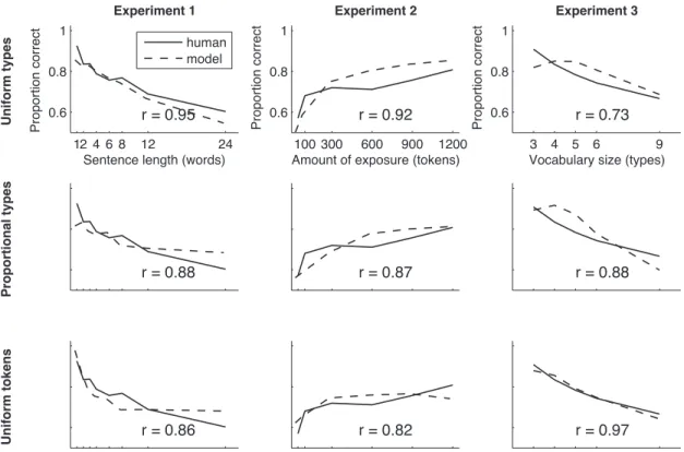
Performance by condition is shown in Figure 1, top left. Participants’ individual data were highly variable, but
● ● ●● ● ● ● ● ●● ● ● ● ● ● ● ● ● ● ● ● ● ● ● ● ● ● ● ● ● ● ● ● ● ● ● ● ● ● ● ● ● ● ● ● ● ● ● ● ● ● ● ● ● ● ● ● ● ● ● ● ● ● ● ● ● ● ● ● ● ● ● ● ● ● ● ● ● ● ● ● ● ● ● ● ● ● ● ● ● ● ● ● ● ● ● ● ● ● ● ● 0 8 16 24 30 40 50 60 70 80 90 100 Experiment 1 sentence length percent correct ● ● ● ● ● ● ● ● ● ● ● ● ● ● ● ● ● ● ● ● ● ● ● ● ● ● ● ● ● ● ● ● ● ● ● ● ● ● ● ● ● ● ● ● ● ● ● ● ● ● ● ● ● ● ● ● ● ● ● ● ● ● ● ● ● ● ● ● ● ● ● ● 0 200 400 600 800 1000 1200 30 40 50 60 70 80 90 100 Experiment 2 number of tokens percent correct ● ● ● ● ● ● ● ● ● ● ● ● ● ● ● ● ● ● ● ● ● ● ● ● ● ● ● ● ● ● ● ● ● ● ● ● ● ● ● ● ● ● ● ● ●● ● ● ● ● ● ● ● ● ●● ● ● ● ● ● ● ● 3 4 5 6 7 8 9 30 40 50 60 70 80 90 100 Experiment 3 number of types percent correct
Figure 1. Data from Experiments 1 – 3. The percentage of test trials answered correctly by each participant (black dots) is plotted by
sentence length, number of tokens, or number of types, respectively. Overlapping points are slightly offset on the horizontal axis to avoid overplotting. Solid lines show means, dashed lines show standard error of the mean, and dotted lines show chance.
showed a very systematic trend in their mean performance across conditions. Although the spread in participants’ per-formance could have been caused by random variation in the phonetic difficulty of the languages we created, the vari-ability was not greater than that observed in previous stud-ies (Saffran, Newport, & Aslin, 1996). Thus, we focused on modeling and understanding mean performance across groups of participants, rather than individual performance.
We analyzed test data using a multilevel (mixed-effect) logistic regression model (Gelman & Hill, 2006). We in-cluded a group-level (fixed) effect of word length and a sep-arate intercept term for each sentence-length condition. We also added a participant-level (random) effect of participant
identity. We fit a separate model with an interaction of word length and sentence length condition but found that it did not significantly increase model fit (χ2(7) = 10.67, p =.15) so we pruned it from the final model.
There was no effect of word length (β = −.00022, z =
.028, p = .99). In contrast, coefficient estimates for sen-tence lengths 1, 2, 3, 4, 6, and 8 were highly reliable (β = 2.31, 1.56, 1.64, 1.39, 1.32, and 1.31 respectively, andz=7.00, 5.16, 5.10, 4.47, 4.24,and 4.20, allp-values
< .0001), while length 12 reached a lower level of signifi-cance (β = .86,z = 2.82, and p = .004). Length 24 was not significant (β = 0.45, z = 1.55, p = .12), indicating that performance in this condition did not differ significantly
from chance. Thus, longer sentences were considerably more difficult to segment.
Experiment 2: Amount of
Exposure
The more exposure to a language learners receive, the eas-ier it should be for them to learn the words. To measure this relationship, we conducted an experiment in which we kept the length of sentences constant but varied the number of to-kens (instances of words) participants heard.
Methods
Participants. We tested 72 MIT students and members of the surrounding community. No participants qualified as outliers by the criteria used in Experiment 1.
Materials. Materials in Experiment 2 were identical to those in Experiment 1, with one exception. We kept the num-ber of words in a sentence constant at four words per sen-tence, but we manipulated the total number of words in the language sample that participants heard. Participants were randomly placed in one of six exposure length conditions (48, 100, 300, 600, 900, and 1200 total tokens). Numbers of tokens were chosen to ensure that they were multiples of both 4 (for sentence length to be even) and 6 (for the fre-quencies of words to be equated). There were a total of 12 participants in each condition.
Procedure. All procedures were identical to those in Ex-periment 1.
Results and Discussion
The results of Experiement 2 are shown in Figure 1, top right. As in Experiment 1, we analyzed the data via a multi-level logistic regression model. There was again no inter-action of condition and word length, so the interinter-action term was again pruned from the model (χ2(5) = 1.69, p = .89). Coefficient estimates for the 48 and 100 conditions did not differ from chance (β = .082 and .39, z = .31 and 1.47, p =.76 and.14). In contrast, coefficients for the other four conditions did reach significance (β = .75, .76, 1.03, and 1.33, z = 2.78, 2.81 3.77,and 4.72, all p-values < .01). Performance rose steeply between 48 tokens and 300 tokens, then was largely comparable between 300 and 1200 tokens.
Experiment 3: Number of Word
Types
The more words in a language, the harder the vocabu-lary of that language should be to remember. All things be-ing equal, three words will be easier to remember than nine words. On the other hand, the more words in a language, the more diverse the evidence that you get. For a transition-finding model, this second fact is reflected in the decreased transition probabilities between words in a larger language, causing part-word distractors to have lower probability. For a chunking model, the same fact is reflected in the increase
in complexity of viable alternative segmentations. For ex-ample, in a three-word language of the type described be-low, hypothesizing boundaries after the first syllable of each word rather than in the correct locations would result in a seg-mentation requiring six words rather than three—a relatively small increase in the size of the hypothesized language. In contrast, a comparable alternative segmentation for a nine-word language would contain 72 “nine-words,” which is a much larger increase over the true solution, and therefore much easier to rule out. Across models, larger languages result in an increase in the amount and diversity of evidence for the correct segmentation.
In our third experiment, we varied the number of distinct word types in the languages we asked participants to learn. If the added cost of remembering a larger lexicon is larger than the added benefit given by seeing a word in a greater diver-sity of contexts, participants should do better in segmenting smaller languages. If the opposite is true, we should expect participants to perform better in larger languages.
Methods
Participants. We tested 63 MIT students and members of the surrounding community. We excluded two participants from the final sample due to performance lower than two standard deviations below the mean performance for their condition.
Materials. Materials in Experiment 3 were identical to those in Experiments 1 and 2, with one exception. We fixed the number of words in each sentence at four and fixed the number of tokens of exposure at 600, but we varied the num-ber of word types in the language, with 3, 4, 5, 6, and 9 types in the languages heard by participants in each of the five con-ditions. Numbers of types were chosen to provide even di-visors of the number of tokens. Note that token frequency increases as the number of types decreases; thus in the 3 type condition, there were 200 tokens of each word, while in the 9 type condition, there were approximately 66 tokens of each word.
Procedure. All procedures were identical to those in Ex-periments 1 and 2.
Results and Discussion
Results of the experiment are shown in Figure 1, bottom. As predicted, performance decreased as the number of types increased (and correspondingly as the token frequency of each type decreased as well). As in Experiments 1 and 2, we analyzed the data via multi-level logistic regression. We again pruned the interaction of word length and condition from the model (χ2(4)=7.06,p=.13). We found no signif-icant effect of word length (β=.031,z=.91,p=.36), but we found significant coefficients for all but the 9 types condi-tion (β=2.12, 1.77, 1.17, .84, and .39,z=5.46, 4.92, 3.17, 2.25, and 1.32, p < .0001 for 3 and 4 types andp =.0015, .025, and .19, for 5, 6, and 9 types, respectively). Thus, per-formance decreased as the number of types increased.
One potential concern about this experiment is that while we varied the number of types in the languages participants learned, this manipulation co-varied with the number of to-kens in the language. To analyze whether the results of exper-iment were due to the number of tokens of each type rather than the number of typesper se, we conducted an additional analysis. We consolidated the data from Experiments 2 and 3 and fit a multi-level model with two main predictors: number of types and number of tokens per type, as well as a binary term for which experiment a participant was in. Because of the relatively large number of levels and because the trend in Experiment 3 was roughly linear, we treated types and tokens per type as linear predictors, rather than as factors as in the previous analyses. (We experimented with adding an inter-action term but found that it did not significantly increase model fit). We found that there was still a negative effect of number of types (β =−.11,z =−2.81, p = .004), even with a separate factor included in the model for the number of tokens per type (β=0.0049,z=5.31,p< .0001). Thus, although the type-token ratio does contribute to the effect we observed in Experiment 3, there is still an independent effect of number of types when we control for this factor.
Model Comparison
In this section, we compare the fit of a number of recent computational proposals for word segmentation to the hu-man experimental results reported above. We do not attempt a comprehensive survey of models of segmentation.1Instead we sample broadly from the space of available models, fo-cusing on those models whose fit or lack of fit to our results may prove theoretically interesting. We first present our ma-terials and comparison scheme; we next give the details of our implementation of each model. Finally, we give results in modeling each of our experiments.
Because all of the models we evaluated were able to seg-ment all experiseg-mental corpora correctly—that is, find the cor-rect lexical items and prefer them to the distractor items— absolute performance was not useful in comparing models. In the terminology introduced above, all models passed the criterion of sufficiency for these simple languages. Instead, we compared models’ fidelity: their fit to human perfor-mance.
Details of simulations
Materials. We compiled a corpus of twelve randomly generated training sets in each of the conditions for each experiment. These training sets were generated identically to those seen by participants and were meant to mimic the slight language-to-language variations found in our training corpora. In addition, because some of the models we eval-uated rely on stochastic decisions, we wanted to ensure that models were evaluated on a range of different training cor-pora. Each training set was accompanied by 30 pairs of test items, the same number of test items as our participants re-ceived. Test items were (as in the human experiments) words in the generating lexicon of the training set or part-word dis-tractors.
We chose syllables as the primary level of analysis for our models. Although other literature has dealt with issues of the appropriate grain of analysis for segmentation models (New-port & Aslin, 2004), in our experiments, all syllables had the same structure (consonant-vowel), so there was no difficulty in segmenting words into syllables. In addition, because we randomized the structure of the lexicon for each language, we chose to neglect syllable-level similarity (e.g., the greater similarity ofka toku than to go). Thus, training materials consisted of strings of unique syllable-level identifiers that did not reflect either the CV structure of the syllable or any syllable-syllable phonetic similarities.
Evaluation. Our metric of evaluation was simple: each model was required to generate a score of some kind for each of the two forced-choice test items. We transformed these scores into probabilities by applying the Luce choice rule (Luce, 1963):
P(a)= S(a)
S(a)+S(b) (1)
whereaandbare test items andS(a) denotes the score ofa under the model. Having produced a choice probability for each test trial, we then averaged these probabilities across test trials to produce an average probability of choosing the correct item at test (which would be equivalent over repeated testing to the corresponding percent correct). We then aver-aged these model runs across training corpora to produce a set of average probabilities for each condition in each exper-iment.
Overall model performance was extremely high. There-fore, rather than comparing models to human data via their absolute deviation (via a measure like mean squared error), we chose to use a simple Pearson correlation coefficient2 to evaluate similarities and differences in the shape of the curves produced when run on experimental data. By evalu-ating model performance in this way, our approach focuses exclusively on the relative differences between conditions rather than models’ absolute fit to human performance, as in Orb´an et al. (2008). Note that the use of a correlation rather than mean squared error is conservative: a model which fails to fit even the shape of human performance will fail even more dramatically when it is evaluated against the absolute level of human performance.
The Luce choice rule is not the only way to combine two scores into a single probability of success on a two-alternative forced-choice trial. In the following discussion of simulation results we will return to the issue of why we chose this particular evaluation metric.
1See e.g. Brent (1999b) and Brent (1999a) for a systematic ex-planation and comparison of models and Goldwater et al. (2009) for more results on recent probabilistic models.
2Pearson (parametric) correlations allow us to fit the shape of curves. We also ran Spearman (rank-order) correlations; the results are comparable, so we have neglected these values for simplicity of comparison.
Models
Transitional probability/Mutual information. As noted in the Introduction, one common approach to segmentation em-ploys simple bigram statistics to measure the relationship be-tween units. To model this approach, we began with the sug-gestion of Saffran, Newport, and Aslin (1996) to use transi-tional probability as a cue for finding word boundaries. We calculated transitional probability (TP) by creating unigram and bigram syllable counts over the training sentences in our corpus with a symbol appended to the beginning and end of each sentence to indicate a boundary. TP was defined with respect to these counts as
T P(st−1,st)=
C(st−1,st) C(st−1)
(2) whereC(st−1) andC(st−1,st) denote the count (frequency) of the syllable st−1 and the string st−1st, respectively. We ad-ditionally investigated point-wise mutual information, a bi-directional statistic that captures the amount that an observer knows about one event given the observation of another:
MI(st−1,st)=log2
C(st−1,st) C(st−1)C(st)
(3) Having computed transitional probability or mutual infor-mation across a corpus, however, there are many ways of converting this statistic into a score for an individual test item. We consider several of these proposals:
1. Local minimum: the lexicon of the language is cre-ated by segmenting the corpus at all local minima in the relevant statistic. Those test items appearing in the lexicon are assigned a score relative to their frequency in the corpus. Words not appearing in the lexicon are assigned a constant score (0 in our simulations).
2. Within-word minimum: words are assigned scores by the minimum value of the statistic for the syllable pairs in that word.
3. Within-word mean: words are assigned scores based on the mean of the relevant statistic.
4. Within-word product: words are assigned scores based on the product of the relevant statistic.
Only some of these options are viable methods for mod-eling variability in our corpus. For instance, the local min-imum method predicts no differences in any of our experi-ments, since frequencies are always equated across items and all conditions have statistical minima between words. There-fore, we evaluated the within-word models: minimum, mean, and product. We found that within-word minimum and within-word product produced identical results (because we always compared words of the same length at test). Within-word mean produced slightly worse results. Therefore we report within-word product results in the simulations that fol-low.3
Both the TP and MI models explicitly took into account the boundaries between sentences. We implemented this feature by assuming that all sentences were bounded by a
start/end symbol, #, and that this symbol was taken into ac-count in the computation of transition ac-counts. Thus, in com-puting counts for the sentence #golabu#, a count would be added for #goas well as forgola. This decision was crucial in allowing these models to have defined counts for transi-tions in Experiment 1’s sentence length 1 condition (other-wise, no word-final syllable would ever have been observed transitioning to any other syllable).
Bayesian Lexical Model. We evaluated the Lexical Model described in Goldwater, Griffiths, and Johnson (2006a); Goldwater et al. (2009). We made use of the simple unigram version (without word-level contextual dependencies) since the experimental corpora we studied were designed to incor-porate no contextual dependencies. The model uses Bayesian inference to identify hypotheses (sequences of word tokens) that have high probability given the observed data d. For any particular hypothesish, the posterior probabilityP(h|d) can be decomposed using Bayes’ Rule, which states that P(h|d)∝P(d|h)P(h). Therefore, optimizingP(h|d) is equiva-lent to optimizing the product of the likelihoodP(d|h) (which tells us how well the data is explained by the hypothesis in question) and the priorP(h) (which tells us how reasonable the hypothesis is, regardless of any data). In this model, the likelihood term is always either 0 or 1 because every se-quence of word tokens is either entirely consistent or entirely inconsistent with the input data. For example, if the input is golabupadoti, then hypothesesgolabu padotiandgo la bu pa dotiare consistent with the input, butlookat thatis not. Consequently, the model need only consider consistent seg-mentations of the input, and of these, the one with the highest prior probability is the optimal hypothesis.
The prior probability of each hypothesis is computed by assuming that words in the sequence are generated from a distribution known as a Dirichlet process. A Dirichlet process is a probabilistic process which generates Dirichlet distributions—discrete distributions over sets of counts—and these Dirichlet distributions are used in the lexical model to parameterize the distribution of word frequencies. The Dirichlet process gives higher probabilities to more concen-trated Dirichlet distributions, corresponding to small lexi-cons with high frequency words. Individual words in the lexicon are then generated according to an exponential dis-tribution, which gives higher probabilities to shorter words.
The probability of the entire sequence of words in the se-quence can be found by multiplying together the probability of each word given the previous words in the sequence. The probability of theith word is given by
P(wi=w|w1. . .wi−1)=
ni−1(w)+αP0(w)
i−1+α (4)
whereni−1(w) is the number of timeswhas occurred in the previousi−1 words,αis a parameter of the model, andP0 3Within-word product also has the advantage of being equiva-lent to word production probability in a Markov model, a fact which makes it an appropriate choice of measure for comparison with the Lexical model in later simulations.
is a distribution specifying the probability that a novel word will consist of the phonemesx1. . .xm:
P0(w=x1. . .xm)= m Y
j=1
P(xj) (5)
According to these definitions, a word will be more probable if it has occurred many times already (ni−1(w) is high), but there is always a small chance of generating a novel word. The relative probability of a novel word decreases as the total number of word tokens (i−1) increases, and novel words are more probable if they are shorter (contain fewer phonemes). The overall effect is a set of soft constraints that can be viewed as constraints on the lexicon: the model prefers seg-mentations that result in lexicons containing a small number of items, each of which is relatively short, and many of which occur very frequently.
The definition given above provides a way to evaluate the probability of any given hypothesis; in order to actu-ally find high-probability segmentations, Goldwater, Grif-fiths, and Johnson (2009) use a Gibbs sampler, a type of algorithm that produces samples from the posterior distribu-tion. The sampler works by randomly initializing all poten-tial word boundary locations (i.e., all syllable boundaries) to either contain a word boundary or not. It then itera-tively modifies the segmentation by choosing whether or not to change its previous decision about each potential word boundary. Each choice is random, but is influenced by the underlying probability model, so that choices that increase the probability of the resulting segmentation are more likely. After many iterations through the data set, this algorithm is guaranteed to converge to producing samples from the pos-terior distribution. Note that, since the goal of Goldwater, Griffiths, and Johnson (2009) was an ideal observer analy-sis of word segmentation, their algorithm is designed to cor-rectly identify high-probability segmentations, but does not necessarily reflect the processes that might allow this in hu-mans. In particular, it is a batch algorithm, requiring all input data to be stored in memory at once. We return to this point later. For more information on Gibbs sampling, see Gelman, Carlin, Stern, and Rubin (2004) and MacKay (2003).
Using the Bayesian lexical model described above, we de-fined the score for a particular word at test to be the posterior probability of the word, estimated by summing over a large number of samples from the posterior. Because the posterior probability of the correct solution was normally so high (in-dicating a high degree of confidence in the solution the model found), we ran the Gibbs sampler using a range of tempera-tures to encourage the model to consider alternate solutions.4 Although this manipulation was necessary for us to be able to evaluate the posterior probability of distractor items, it had relatively little effect on the results across a large range of temperatures (2 – 20). We therefore report results from tem-perature=2. The model had one further parameter: theα parameter of the Dirichlet process, which we kept constant at the value used in Goldwater et al. (2009).
In the language of the introduction, the Lexical model is a chunking model, rather than a transition-finding model:
though its inference algorithm works over boundary posi-tions, its hypotheses are sequences of chunks (words) and the measures with which it evaluates hypotheses are stated in terms of these chunks (how many unique chunks there are, their frequencies, and their lengths).
MI Clustering. We evaluated the mutual information-based clustering model described in Swingley (2005). This model is a clustering model which calculates n-gram statis-tics and pointwise mutual information over a corpus, then takes as words those strings which exceed a certain threshold value both in their frequency and in the mutual information of their constituent bisyllables. Unlike our versions of the TP and MI models, the MI Clustering model looks for coherent chunks which satisfy its criteria of frequency and mutual in-formation (and it evaluates these criteria for every possible chunk in the exposure corpus). Thus, like the Lexical model, it is a chunking model rather than a transition-finding model. In order to run the model on the language of our experi-ment, we added support for four-syllable words by analogy to three-syllable words. We then defined the score of a string under the model (given some input corpus) as the maximum threshold value at which that string appeared in the lexicon found by the model. In other words, the highest-scoring strings were those that had the highest percentile rank both in mutual information and in frequency.
PARSER. We implemented the PARSER model described in Perruchet and Vinter (1998) and Perruchet and Vinter (2002).5 PARSER is organized around a lexicon, a set of words and scores for each word. The model receives input sentences, parses them according to the current lexicon, and then adds sequences to the lexicon at random from the parsed input. Each lexical item decays at a constant rate and similar items interfere with each other. The model as described has six parameters: the maximum length of an added sequence, the weight threshold for a word being used to parse new sequences, the forgetting and interference rates, the gain in weight for reactivation, and the initial weight of new words. Because of the large number of parameters in this model, it was not possible to complete an exhaustive search of the parameter space; however, we experimented with a variety of different combinations of interference and forgetting rates and maximum sequence lengths without finding any major differences in forced-choice performance. We therefore re-port results using the same parameter settings used in the ini-tial paper.
We made one minor modification to the model to allow it to run on our data: our implementation of the model iterated through each sentence until reaching the end and then began 4Temperature is a parameter which controls the degree to which the Gibbs sampler prefers more probable lexicons, with higher temperature indicating greater willingness to consider lower-probability lexicons. See Kirkpatrick, Gelatt, and Vecchi (1983) for more details.
5We also thank Pierre Perruchet for providing a reference im-plementation of PARSER, whose results were identical to those we report here.
anew at the beginning of the next sentence—thus, it could not add sentence-spanning chunks to its lexicon.
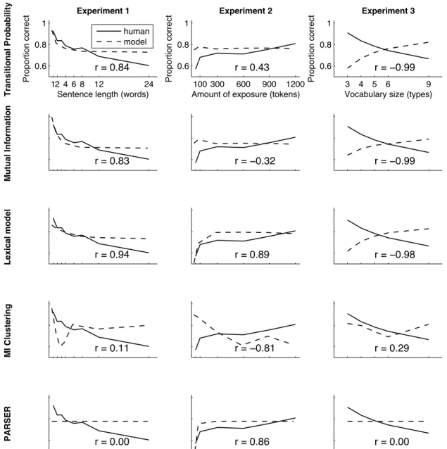
Comparison results
Figure 2 shows the performance of each model plotted side-by-side with the human performance curves shown in Figure 1. For convenience we have adjusted all the data from each model via a single transformation to match their scale and intercept to the mean human performance. This adjust-ment does not affect the Pearsonrvalues given in each sub-plot, which are our primary method of comparison. We dis-cuss the model results for each experiment in turn, then end by considering effects of word length on model performance. Experiment 1. Most models replicated the basic pattern of performance in Experiment 1, making fewer errors (or assigning less probability to distractors) when words were presented alone or in shorter sentences. However, there were differences in how well the models fit the quantitative trend. Both the TP and MI models showed a relatively large de-crease in performance from single-word sentences to two-word sentences. In the TP model, this transition is caused by the large difference between distractors which have a score of 0 (in the single-word sentences) and distractors which have a score of 1/10 (in the two word sentences—since every other word is followed by one of 5 different words). However, the relative difference in probabilities between sentences with 12 words and sentences with 24 words was very small, as re-flected in the flatness of both the TP and MI curves. This trend did not exactly match the pattern in the human data, where performance continued to decrease from 12 to 24.
Compared to the TP and MI models, the Lexical Model showed a slightly better fit to the human data, with per-formance decreasing more gradually as sentence length in-creased. The Lexical Model’s increased difficulty with longer sentence lengths can be explained as follows. The model is designed to assign a probability to every possible segmentation of a given input string. Although the prob-abilities assigned to incorrect segmentations are extremely low, longer sentences have a much larger number of possi-ble segmentations. Thus, the total probability of all incorrect segmentations tends to increase as sentence length increases, and the probability of the correct segmentation must drop as a result. Essentially, the effects of sentence length are mod-eled by assuming competition between correct and incorrect segmentations.
The MI Clustering model in this (and both other) experi-ments produced an extremely jagged curve, leading to a very low correlation value. The reason for this jaggedness was simple: since the model relies on percentile rankings of fre-quency rather than raw frequencies, its performance varied widely with very small changes in frequency (e.g., those in-troduced by the slight differences between input corpora in our studies). Because the model is deterministic, this noise could not be averaged out by multiple runs through the input corpus.
PARSER failed to produce the human pattern of results. In any given run, PARSER assigned the target a non-zero
(of-ten high) score and the distractor a score of 0 or very close to zero, producing a flat response curve across conditions. In order to verify that this was not an artifact of the relatively small number of simulations we performed, we ran a second set of simulations with 100 independent PARSER runs for each training set. The results of these simulations were qual-itatively very similar across all three experiments despite the integration of 1200 datapoints for each point on each curve. We return to the issue of PARSER’s performance in the dis-cussion on target and distractor probabilities.
Experiment 2. The TP and MI models, which performed relatively well in Experiment 1, failed to produce the pattern of gradual learning in Experiment 2. This result stems from the fact that both models producepoint estimatesof descrip-tive statistics. These point estimates require very little data to converge to their eventual values. Regardless of whether the models observe 300 or 1200 sentences, the transitional probability they find between any two words will be very close to 1/5 (since any word can be followed by any other except itself). This same fact also explains the relatively flat performance of the MI Clustering model, though this model’s high performance with very little input reflects the likelihood of not having observed the distractor items even once at the beginning of exposure.
In contrast, both the Lexical Model and PARSER suc-ceeded in fitting the basic pattern of performance in this experiment. Although PARSER is an online model which walks through the data in a single pass and the Lexical Model is a batch model which processes all the available data at once, both models incorporate some notion that more data provides more support for a particular hypothesis. In the Lexical Model, which evaluates hypothesized lexicons by their parsimony relative to the length of the corpus that is generated from them, the more data the model observes, the more peaked its posterior probability distribution is. In PARSER, the more examples of a particular word the model sees in the exposure corpus, the larger its score in the lexicon (and the longer it will take to forget). Another way of stating this result: more examples of any concept make that concept faster to process and easier to remember.
Experiment 3. The results of the model comparison on Experiment 3 were striking. No model succeeded in cap-turing the human pattern of performance in this experiment. MI Clustering and PARSER were uncorrelated with human performance. All three of the other models showed a clear trend in the opposite direction of the pattern shown by the human participants. These models performed better on the languages with larger numbers of word types for the same reason: languages with a larger number of word types had distractors that were less statistically coherent. For exam-ple, a language with only three types has a between-word TP of 1/2 while a language with nine types has a far lower between-word TP of 1/8, leading to part-words with very low within-word TP scores.
Put another way, the advantage that human participants gained from the clearer statistics of the larger language did
12 4 6 8 12 24 0.6
0.8 1
Experiment 1
Transitional Probability Sentence length (words)
Proportion correct r = 0.84 human model Mutual Information r = 0.83 Lexical model r = 0.94 MI Clustering r = 0.11 PARSER r = 0.00 100 300 600 900 1200 0.6 0.8 1 Experiment 2 r = 0.43 Amount of exposure (tokens)
Proportion correct r = ï0.32 r = 0.89 r = ï0.81 r = 0.86 3 4 5 6 9 0.6 0.8 1 Experiment 3 r = ï0.99
Vocabulary size (types)
Proportion correct
r = ï0.99
r = ï0.98
r = 0.29
r = 0.00
Figure 2. Comparison of model results to human data for Experiments 1 – 3. All results from each model are adjusted to the same scale
and intercept as human data to facilitate comparison (this manipulation does not affect the Pearson correlation coefficient given at the bottom of each subplot). Models are slightly offset in the horizontal axis to avoid overplotting.
not outweigh the disadvantage of having to remember more words and having to learn them from fewer exposures. The TP, MI, and Lexical Models, in contrast, all weighted the clearer statistics of the language far more heavily than the decrease in the number of tokens for each word type.
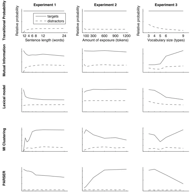
Probabilities of targets and distractors
Models differed widely in whether conditions which pro-duced lower performance did so because targets were as-signed lower scores, or because distractors were asas-signed higher scores. This section discusses these differences in the context of previous work and our decision to use a choice
rule which includes both target and distractor probabilities. Figure 3 shows the relative probabilities of targets and dis-tractors for each experiment and model. We have chosen not to give vertical axis units since the scale of scores for each model varies so widely; instead, this analysis illustrates the qualitative differences between models.
The transitional probability model produces different pat-terns of performance only because the probabilities of dis-tractors vary from condition to condition. As noted pre-viously, in the languages we considered, transitions within words are always 1; therefore overall performance depends on the TP at word boundaries. In contrast, because mutual
12 4 6 8 12 24 Experiment 1
Transitional Probability Sentence length (words)
Relative probability targets distractors Mutual Information Lexical model MI Clustering PARSER 100 300 600 900 1200 Experiment 2
Amount of exposure (tokens)
Relative probability 3 4 5 6 9
Experiment 3
Vocabulary size (types)
Relative probability
Figure 3. Relative probabilities of target and distractor items for the models we evaluated. Vertical axis is scaled separately for each
row. To illustrate trends in the Lexical model, results are plotted from temperature 20 (though results were qualitatively similar across all temperatures).
information is normalized bidirectionally (and hence takes into account more global properties of the language), target MI changed as well as distractor MI. Nonetheless, the Luce choice probabilties for MI and TP were quite similar, sug-gesting that the differences in the MI model were not sub-stantive.
Considering target and distractor probabilities for the Lex-ical model we see several interesting features. First, ef-fects in Experiments 1 and 2 seem largely (though not en-tirely) driven by target probability. Although there is some increase in distractor probability in Experiment 1, targets become considerably less probable as sentence lengths
in-crease. Likewise in Experiment 2, distractor probabilities remain essentially constant, but the greater amount of expo-sure to target words increases target probabilities. Experi-ment 3 shows a different pattern, however: target probabili-ties match human performance, decreasing as word lengths increase. But distractor probabilities decrease more slowly than target probabilities, canceling this effect and leading to the overall reversal seen in Figure 3. Put another way: it is not that targets increase in probability as languages grow in vocabulary size. Instead, the effects we observed in the Lexical model in Experiment 3 are due to the probabilities of distractors relative to targets. (Correlations between
Lexi-cal Model target probabilities and human performance were r=.82,.89, and.96, respectively).
The MI Clustering model showed patterns of target scores that were the reverse of human performance for all three experiments, though in Experiment 1 changes in distractor score were large enough to reverse this trend. For the other two experiments we saw only limited effects of distractor probability.
Target and distractor probabilities for PARSER were re-vealing. Target probabilities for all three experiments fol-lowed the same qualitative pattern as human performance: decreasing in Experiments 1 and 3 and increasing in Ex-periment 2. Thus, it was purely the fact that PARSER as-signed no score to distractors that prevented it from captur-ing general trends in human performance. Were correlations assessed with target scores alone, PARSER would correlate atr =.92,.84, and.89 with human performance across the three experiments, respectively (comparable to the level of the Lexical Model target probabilities and to the resource-limited probabilistic models discussed in the next section).
Overall, this analysis suggests that the Luce choice rule we used (and that it weighted target and distractor proba-bilities equivalently) led to the patterns we observed in the comparison with human performance. This result begs the question of why we chose the Luce choice rule in particular. The key argument for considering distractor probability in evaluating model performance is given by the experimen-tal data reported in Saffran, Newport, and Aslin (1996). In Experiment 1, Saffran et al. trained two groups of human participants on the same exposure corpus but tested them on two different sets of materials. The targets in each set were the legal words of the corpus that the participants had been exposed to, but one group heard non-word distractors— concatenations of syllables from the language that had not been seen together in the exposure corpus—while the other group heard part-word distractors that (comparable to our distractors) included a two-syllable substring from a legal word in the corpus. Performance differed significantly be-tween these two conditions, with participants rejecting non-words more than part-non-words. These results strongly suggest that human learners are able to assign probabilities to distrac-tors and that distractor probabilities matter to the accuracy of human judgments at test.
Distractor probabilities could be represented in a number of ways that would be consistent with the current empiri-cal data. For example, human learners could keep track of a discrete lexicon like the one learned by PARSER, but sim-ply include more possible strings in it than those represented by PARSER in our simulations. On this kind of account, the difficulty learners had in the part-word condition of Saf-fran et al.’s experiment would be caused by confusion over the part words (since non-words would not be represented at all). This kind of story would still have to account for the difficulty of the non-word condition, though, since most participants were still not at ceiling. On the other hand, a TP-style proposal (much like the probabilistic DM-TP model proposed in the next section) would suggest that participants could evaluate the relative probabilities of any string in the
language they heard. Current empirical data do not distin-guish between these alternatives but they do strongly suggest that human learners represent distractor probabilities in some form.
Discussion
Under the evaluation scheme we used, no model was able to fit even the relative pattern of results in all three experi-ments. In particular, no model produced a similar trend to hu-man data in Experiment 3, and hu-many failed to in Experiment 2 as well. Although some models assigned relative probabil-ities to target items that matched human performance, when distractor probabilities were considered, model performance diverged sharply from humans.
We speculate that the match and mismatch between mod-els and data is due to the failure of this first set of modmod-els to incorporate any notion of resource limitations. Human learn-ers are limited in their memory for the data they are exposed to—they cannot store hundreds of training sentences—and for what they have learned—a large lexicon is more difficult to remember than a smaller one. This simple idea accounts for the results of both Experiment 2 and Experiment 3. In Experiment 2, if participants are forgetting much of what they hear, hearing more examples will lead to increased per-formance. In Experiment 3, although larger languages had clearer transition statistics, they also had more words to re-member. The next section considers modifications to two probabilistic models (the Lexical Model and a modified ver-sion of the TP model) to address human memory limitations.
Adding Resource Constraints to
Probabilistic Models
Memory limitations provide a possible explanation for the failure of many models to fit human data. To test this hy-pothesis, the last section of the paper investigates the issue of adding memory limitations to models of segmentation. We explore two methods. The first,evidence limitation, imple-ments memory limitations as a reduction in the amount of the evidence available to learners. The second,capacity limita-tion, implements memory limitations explicitly via imposing limits on models’ internal states.
For this next set of simulations, we narrow the field of models we consider, looking only at probabilistic genera-tive models. These models are “Bayesian models” because they are often stated in terms of a decomposition into a prior over some hypothesis space and a likelihood over data given hypotheses, allowing the use of a family of Bayesian infer-ence techniques for finding the posterior distribution of hy-potheses given some observed data. We choose this model-ing framework because it provides a common vocabulary and set of tools for stating models with different representations and performing inference in these models; hence modeling insights from one model can easily be applied to another model. (The results of Orb´an et al., 2008, provide one ex-ample of the value of comparing models posed in the same framework).
The only probabilistic generative model in our initial com-parison was the Lexical Model. However, standard transi-tional probability models are closely related to probabilistic generative models. Therefore, before beginning this investi-gation we rewrite the standard transitional probability model, modifying it so that it is a standard Bayesian model which can be decomposed into a prior probability distribution and a likelihood of the data given the model. We refer to this new model as the DM-TP (Dirichlet-multinomial TP) model because it uses a Dirichlet prior distribution and multinomial likelihood function.
Modifications to the TP model
As we defined it above, the transitional probability model includes no notion of strength of evidence. It will make the same estimate of TP whether it has observed a given set of transitions once or 100 times. This property comes from the fact that Equation 2 is a maximum-likelihood estima-tor, a formula which gives the highest probability estimate for a particular quantity regardless of the confidence of that estimate. In contrast, a Bayesian estimate of a particular quantity interpolates between the likelihood of a particular value given the data and the prior probability of that value. With very little data, the Bayesian estimate is very close to the prior. In the presence of more data, the Bayesian esti-mate asymptotically approaches the maximum likelihood es-timate. In this section we describe a simple Bayesian version of the TP model which allows it to incorporate some notion of evidence strength.
In order to motivate the Bayesian TP model we propose, we briefly describe the equivalence of the TP model to sim-ple Markov models that are commonly used in computational linguistics (Manning & Sch¨utze, 1999; Jurafsky & Martin, 2008). A Markov model is simply a model which makes a Markov, or independence, assumption: the current observa-tion depends only on thenprevious observations and is inde-pendent of all others. In this way of viewing the model, each syllable is a state in a finite-state machine: a machine com-posed of set of states which emit characters, combined with transitions between these states. In such a model, the proba-bilities of a transition from each state to each other state must be learned from the data. The maximum-likelihood estimate of the transition probabilities from this model is the same as we gave previously in Equation 2: for each state we count the number of transitions to other states and then normalize. One weakness of Markov models is their large number of parameters, which must be estimated from data. The num-ber of parameters in a standard Markov model is exponen-tial, growing as mn, wherem is the number of states (dis-tinct syllables) andnis the “depth” of the model (the number of states that are taken into account when computing tran-sition probabilities—here,n = 2 because we consider pairs of syllables). Because of this problem, a large amount of the literature on Markov models has dealt with the issue of how to estimate these parameters effectively in the absence of the necessary quantity of data (the “data sparsity” prob-lem). This process is often referred to as “smoothing” (Chen
& Goodman, 1999).
After observing only a single transition (say in the se-quencegola) a standard maximum-likelihood TP model cal-culates that the transition fromgotolahappens with prob-ability 1 and that there is no other syllable in future expo-sure that will ever followgo. This tendency to jump to con-clusions has the consequence of severely limiting the abil-ity of unsmoothed Markov models to generalize from lim-ited amounts of data. Instead, they tend to overfit whatever data they are presented with, implicitly assuming that the ev-idence that has been presented is perfectly representative of future data. (This is precisely the phenomenon that we saw in the failure of the TP model in Experiment 2: even with a small amount of evidence, the model overfit the data, learn-ing the transition probabilities perfectly.)
One simple way to deal with this issue of unseen fu-ture data is to estimate transitions using Bayesian inference. Making Bayesian inferences consists of assuming some prior beliefs about the transition structure of the data—in this case, the conservative belief that transitions are uniform—that are gradually modified with respect to observed data. To do this, we assume that transitions are samples from a multinomial distribution. Rather than estimating the maximum-likelihood value for this distribution from counts (as in Equation 2), we add a prior distribution over possible values of P(st−1,st). The form of this prior is a Dirichlet distribution with parame-terα. Because of the conjugacy of the Dirichlet and multino-mial distributions (Gelman et al., 2004), we can express the new estimate of transition probability simply by adding a set of “pseudo-counts” of magnitudeαto each estimate:
P(st−1,st)=
C(st−1,st)+α P
s0∈S(C(st−1,s0)+α)
. (6)
Under this formulation, even when a particular syllableshas not been observed, its transitional probability is not zero. In-stead, it has some smoothed base value that is determined by the value ofα.6
Note that asαbecomes small, the DM-TP model reduces to the TP model that we already evaluated above. The Ap-pendix gives results on the DM-TP model’s fit to all three experiments over a wide range of values ofα. In the next sec-tions, however, we investigate proposals for imposing mem-ory limitations on the DM-TP and Lexical models.
Modeling memory e
ff
ects by evidence limitation
One crude way of limiting models’ memory is never to provide data to be remembered in the first place. Thus, the first and most basic modification we introduced to the Lex-ical and TP models was simply to limit the amount of evi-dence available to the models.
6Adding this prior distribution to a TP model creates what is known in computational linguistics as a smoothed model, equiva-lent to the simple and common “add-delta” smoothing described in Chen and Goodman (1999)’s study of smoothing techniques. For more detail on the relationship between Dirichlet distributions and smoothing techniques see MacKay and Peto (1994), Goldwater, Griffiths, and Johnson (2006b), and Teh (2006).
12 4 6 8 12 24 0.6 0.8 1 Experiment 1 DM-TP 4% data
Sentence length (words)
Proportion correct r = 0.82 human model Lexical - 4% data r = 0.88 100 300 600 900 1200 0.6 0.8 1 Experiment 2 r = 0.92
Amount of exposure (tokens)
Proportion correct r = 0.85 3 4 5 6 9 0.6 0.8 1 Experiment 3 r = 0.96
Vocabulary size (types)
Proportion correct
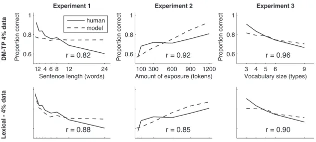
r = 0.90
Figure 4. Comparison of Bayesian transitional probability model and Lexical Model, both trained with 4% of the original dataset, to human data. Model results are offset, scaled, and adjusted to the same intercept as human data to facilitate comparison, as in Figure 2.
Methods. We conducted these simulations by running both the DM-TP and the Lexical Model on a new set of ex-perimental materials. These materials were generated identi-cally to the experimental materials in the previous section ex-cept that we presented the models with only 4% of the origi-nal quantity of data. (We chose 4% to be the smallest amount of data that would minimize rounding errors in the number of sentences in each exposure corpus). For example, in Ex-periment 1, models were presented with 24 (rather than 600) word tokens, distributed in 24 1-word sentences, 12 2-word sentences, 8 3-word sentences, etc. The number of tokens was reduced similarly in Experiments 2 and 3 while holding all other details of the simulations (including the number of types) constant from the original model comparison.
Results. We evaluated performance across a range of val-ues ofαfor the DM-TP model and across a range of temper-atures for the Lexical Model. As before, although there was some variability between simulations, all temperatures of 2 and above produced substantially similar results. In contrast, results on Experiment 3 (but not the other two experiments) varied considerably with different values ofα. We return to this issue below.
Results forα=32 and temperature 3 are plotted in Figure 4. For these parameter settings, performance in the two mod-els was very similar across all three experiments (r = .90), and both models showed a relatively good fit to the data from all three conditions. In the Appendix, we further explore the
αparameter and its role in fitting human data. In Experi-ment 1, both models captured the general trend, although the DM-TP model showed this pattern only within an extremely compressed range. In Experiment 2, both models captured the basic direction of the trend but not its asymptotic, decel-erating shape. In Experiment 3, in contrast to the results of our first set of simulations, both models captured the trend
of decreasing performance with increasing vocabulary size (although they did not exactly match the decrease in perfor-mance between languages with 3 and 4 words).
Discussion. Why did limiting the evidence available to the models lead to success in fitting the decreasing trend in human performance in Experiment 3? Performance in Ex-periment 3 for both models comes from a tradeoffbetween two factors. The first factor is the decreasing statistical co-herence of distractors as the number of types in the language increases. With 3 types, distractors (part-words) contain at most one transition with probability 1/2; with 9 types in contrast, distractors contain a transition with probability 1/8. The second factor at work is the decreasing number of to-kens of each type in conditions with more types. A smaller number of tokens means less evidence about any particular token.
In the original simulations, the first factor (statistical co-herence) dominated the second (type/token ratio) for both the Lexical Model and the TP model. With its perfect memory, the Lexical Model had more than enough evidence to learn any particular type; thus the coherence of the distractors was a more important factor. Likewise, the point estimates of transition probability in the TP model were highly accurate given the large number of tokens. In contrast, in the reduced-data simulations, the balance between these two factors was different. For instance, in the Lexical Model, while a larger vocabulary still lead to lower coherence within the distrac-tors, this factor was counterbalanced by the greater uncer-tainty about the targets (because of the small number of ex-posures to any given target). In the DM-TP model, the same principle was at work. Because of the prior expectation of uniform transitions, conditions with more types had a small enough number of tokens to add uncertainty to the estimates of target probability. Thus, for both Bayesian models, less