American Mathematical Society

TEX

Michael Downes

American Mathematical Society

Version 1.07 (2000/07/19)

1. Introduction This is a concise summary of recommended features in LA_{TEX and a}

couple of extension packages forwriting math formulas. Readers needing greater depth of detail are referred to the sources listed in the bibliography, especially [Lamport], [LaTeX-U], [AMUG], [LaTeX-F], [LaTeX-G], and [GMS]. A certain amount of familiarity with standard LA_{TEX terminology is assumed; if your memory needs refreshing on the L}A_{TEX meaning of} command,optional argument,environment,package, and so forth, see [Lamport].

The features described here are available to you if you use LA_{TEX with two extension}

packages published by the American Mathematical Society: amssymbandamsmath. Thus, the source file for this document begins with

\documentclass{article} \usepackage{amssymb,amsmath}

Theamssymbpackage might be omissible for documents whose math symbol usage is rela-tively modest; the easiest way to test this is to leave out theamssymbreference and see if any math symbols in the document stop working.

Many noteworthy features found in other packages are not covered here; see Section 9.

2. Inline math formulas and displayed equations

2.1. The fundamentals Entering and leaving math mode in LA_{TEX is normally done with}

the following commands and environments.

inline formulas displayed equations $. . . $ \(. . . \) \[...\] unnumbered \begin{equation*} . . . \end{equation*} unnumbered \begin{equation} . . . \end{equation} automatically numbered

Note. Alternative environments\begin{math}. . .\end{math},\begin{displaymath}. . .\end{displaymath}

are seldom needed in practice. Using the plain TEX notation$$. . . $$for displayed equations is not rec-ommended. Even though it is not expressly forbidden in LA_{TEX, it interferes with the proper operation of} various features such as thefleqnoption.

Environments for handling equation groups and multi-line equations are shown in Table 1.

2.2. Automatic numbering and cross-referencing To get an auto-numbered

equa-tion, use theequationenvironment; to assign a label for cross-referencing, use the\label

command:

\begin{equation}\label{reio} ...

\end{equation}

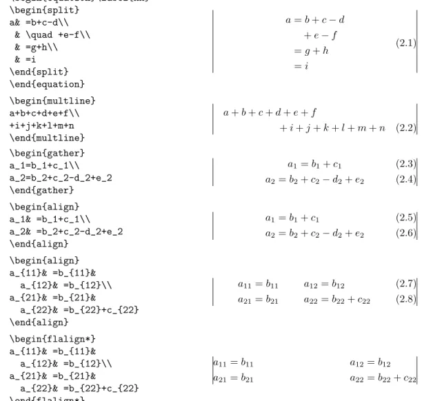
Table 1: Multi-line equations and equation groups (vertical lines indicating nominal mar-gins).

\begin{equation}\label{xx} \begin{split}

a& =b+c-d\\ & \quad +e-f\\ & =g+h\\ & =i \end{split} \end{equation} a=b+c−d +e−f =g+h =i (2.1) \begin{multline} a+b+c+d+e+f\\ +i+j+k+l+m+n \end{multline} a+b+c+d+e+f +i+j+k+l+m+n (2.2) \begin{gather} a_1=b_1+c_1\\ a_2=b_2+c_2-d_2+e_2 \end{gather} a1=b1+c1 (2.3) a2=b2+c2−d2+e2 (2.4) \begin{align} a_1& =b_1+c_1\\ a_2& =b_2+c_2-d_2+e_2 \end{align} a1=b1+c1 (2.5) a2=b2+c2−d2+e2 (2.6) \begin{align} a_{11}& =b_{11}& a_{12}& =b_{12}\\ a_{21}& =b_{21}& a_{22}& =b_{22}+c_{22} \end{align} a11=b11 a12=b12 (2.7) a21=b21 a22=b22+c22 (2.8) \begin{flalign*} a_{11}& =b_{11}& a_{12}& =b_{12}\\ a_{21}& =b_{21}& a_{22}& =b_{22}+c_{22} \end{flalign*} a11=b11 a12=b12 a21=b21 a22=b22+c22

Note 1. Thesplitenvironment is something of a special case. It is a subordinate environment that can be used as the contents of anequationenvironment or the contents of one “line” in a multiple-equation structure such asalignorgather.

Note 2. Theeqnarrayandeqnarray*environments described in [Lamport] are not recommended because they produce inconsistent spacing of the equal signs and make no attempt to prevent overprinting of the equation body and equation number.

To get a cross-reference to an auto-numbered equation, use the\eqrefcommand:

... using equations \eqref{ax1} and \eqref{bz2}, we can derive ...

The above example would produce something like using equations (3.2) and (3.5), we can derive

In other words,\eqref{ax1}is equivalent to(\ref{ax1}).

To give your equation numbers the form m.n (section-number.equation-number), use the\numberwithincommand in the preamble of your document:

\numberwithin{equation}{section}

For more details on custom numbering schemes see [Lamport,§6.3,§C.8.4].

The subequations environment provides a convenient way to number equations in a group with a subordinate numbering scheme. For example, supposing that the current equation number is 2.1, write

\begin{equation}\label{first} a=b+c

\end{equation}

some intervening text

\begin{subequations}\label{grp} \begin{align} a&=b+c\label{second}\\ d&=e+f+g\label{third}\\ h&=i+j\label{fourth} \end{align} \end{subequations} to get a=b+c (2.9)

some intervening text

a=b+c (2.10a)

d=e+f+g (2.10b)

h=i+j (2.10c)

By putting a \label command immediately after \begin{subequations} you can get a reference to the parent number;\eqref{grp}from the above example would produce (2.10) while\eqref{second}would produce (2.10a).

3. Math symbols and math fonts

3.1. Classes of math symbols The symbols in a math formula fall into different classes

that correspond more or less to the part of speech each symbol would have if the formula were expressed in words. Certain spacing and positioning cues are traditionally used for the different symbol classes to increase the readability of formulas.

Class

number Mnemonic

Description

(part of speech) Examples

0 Ord simple/ordinary (“noun”) A0 Φ∞

1 Op prefix operator P Q R

2 Bin binary operator (conjunction) +∪ ∧

3 Rel relation/comparison (verb) =<⊂

4 Open left/opening delimiter ( [{ h

5 Close right/closing delimiter ) ]} i

Note 1. The distinction in TEX between class 0 and an additional class 7 has to do only with font selection issues and is immaterial here.

Note 2. Symbols of class Bin, notably the minus sign−, are automatically coerced to class 0 (no space) if they do not have a suitable left operand.

The spacing for a few symbols follows tradition instead of the general rule: although / is (semantically speaking) of class 2, we writek/2 with no space around the slash rather thank /2. And comparep|qp|q(no space) with p\mid qp|q(class-3 spacing).

The proper way to define a new math symbol is discussed in LA_{TEX 2ε font selection} [LaTeX-F]. It is not really possible to give a useful synopsis here because one needs first to understand the ramifications of font specifications.

3.2. Some symbols intentionally omitted here The following math symbols that

are mentioned in the LA_{TEX book [Lamport] are intentionally omitted from this discussion}

because they are superseded by equivalent symbols when theamssymb package is loaded. If you are using theamssymbpackage anyway, the only thing that you are likely to gain by using the alternate name is an unnecessary increase in the number of fonts used by your document.

\Box, see \square \Diamond, see \lozenge_♦ \leadsto, see \rightsquigarrow

\Join, see \bowtie./

\lhd, see \vartriangleleftC

\unlhd, see \trianglelefteqE

\rhd, see \vartriangleright_B \unrhd, see \trianglerighteq_D

3.3. Latin letters and Arabic numerals The Latin letters are simple symbols, class 0.

The default font for them in math formulas is italic.

A B C D E F G H I J K L M N O P Q R S T U V W X Y Z a b c d e f g h i j k l m n o p q r s t u v w x y z

When adding an accent to aniorjin math, dotless variants can be obtained with\imath

and\jmath:

ı\imath \jmath ˆ\hat{\jmath}

Arabic numerals 0–9 are also of class 0. Their default font is upright/roman. 0 1 2 3 4 5 6 7 8 9

3.4. Greek letters Like the Latin letters, the Greek letters are simple symbols, class 0. For obscure historical reasons, the default font for lowercase Greek letters in math formu-las is italic while the default font for capital Greek letters is upright/roman. (In other fields such as physics and chemistry, however, the typographical traditions are somewhat different.) The capital Greek letters not present in this list are the letters that have the same appearance as some Latin letter: A for Alpha, B for Beta, and so on. In the list of lowercase letters there is no omicron because it would be identical in appearance to Latino. In practice, the Greek letters that have Latin look-alikes are seldom used in math formulas,

to avoid confusion. Γ\Gamma ∆\Delta Λ\Lambda Φ\Phi Π\Pi Ψ\Psi Σ\Sigma Θ\Theta Υ\Upsilon Ξ\Xi Ω\Omega α\alpha β \beta γ \gamma δ\delta \epsilon ζ \zeta η \eta θ \theta ι\iota κ\kappa λ\lambda µ\mu ν \nu ξ\xi π\pi ρ\rho σ\sigma τ \tau υ \upsilon φ\phi χ \chi ψ\psi ω \omega z\digamma ε\varepsilon κ \varkappa ϕ\varphi $ \varpi %\varrho ς \varsigma ϑ\vartheta

3.5. Other alphabetic symbols These are also class 0.

ℵ\aleph i\beth k\daleth ג\gimel { \complement ` \ell ð \eth ~\hbar }\hslash f\mho ∂ \partial ℘\wp s\circledS k\Bbbk `\Finv a\Game =\Im <\Re

3.6. Miscellaneous simple symbols These symbols are also of class 0 (ordinary) which

means they do not have any built-in spacing. #\# &\& ∠\angle 8\backprime F\bigstar \blacklozenge \blacksquare N\blacktriangle H\blacktriangledown ⊥\bot ♣\clubsuit \diagdown \diagup ♦\diamondsuit ∅\emptyset ∃\exists [\flat ∀\forall ♥\heartsuit ∞\infty ♦\lozenge ]\measuredangle ∇\nabla \\natural ¬\neg @\nexists 0\prime ]\sharp ♠\spadesuit ^\sphericalangle \square √ \surd >\top 4\triangle O\triangledown ∅\varnothing

Note 1. A common mistake in the use of the symbols and # is to try to make them serve as binary operators or relation symbols without using a properly defined math symbol command. If you merely use the existing commands\squareor\#the inter-symbol spacing will be incorrect because those commands produce a class-0 symbol.

3.7. Binary operator symbols ∗ * ++ − -q\amalg ∗ \ast Z\barwedge \bigcirc 5\bigtriangledown 4\bigtriangleup \boxdot \boxminus \boxplus \boxtimes • \bullet ∩\cap e\Cap · \cdot \centerdot ◦ \circ ~\circledast }\circledcirc \circleddash ∪\cup d\Cup g \curlyvee f \curlywedge †\dagger ‡\ddagger \diamond ÷\div >\divideontimes u\dotplus [ \doublebarwedge m\gtrdot | \intercal h\leftthreetimes l\lessdot n\ltimes ∓\mp \odot \ominus ⊕\oplus \oslash ⊗\otimes ±\pm i\rightthreetimes o\rtimes \ \setminus r\smallsetminus u\sqcap t\sqcup ?\star ×\times /\triangleleft .\triangleright ]\uplus ∨\vee Y\veebar ∧\wedge o\wr

Synonyms: ∧\land,∨\lor,d\doublecup,e\doublecap

3.8. Relation symbols: <= > ∼and variants

<< == >> ≈\approx u\approxeq \asymp v\backsim w\backsimeq l\bumpeq m\Bumpeq $\circeq ∼ =\cong 2\curlyeqprec 3\curlyeqsucc . =\doteq +\doteqdot P\eqcirc h\eqsim 1\eqslantgtr 0\eqslantless ≡\equiv ;\fallingdotseq ≥\geq =\geqq >\geqslant \gg ≫\ggg \gnapprox \gneq \gneqq \gnsim '\gtrapprox R\gtreqless T\gtreqqless ≷\gtrless &\gtrsim \gvertneqq ≤\leq 5\leqq 6\leqslant /\lessapprox Q\lesseqgtr S\lesseqqgtr ≶\lessgtr .\lesssim \ll ≪\lll \lnapprox \lneq \lneqq \lnsim \lvertneqq \ncong 6 =\neq \ngeq \ngeqq \ngeqslant ≯\ngtr \nleq \nleqq \nleqslant ≮\nless ⊀\nprec \npreceq \nsim \nsucc \nsucceq ≺\prec w\precapprox 4\preccurlyeq \preceq \precnapprox \precneqq \precnsim -\precsim :\risingdotseq ∼\sim '\simeq \succ v\succapprox <\succcurlyeq \succeq \succnapprox \succneqq \succnsim %\succsim ≈\thickapprox ∼\thicksim ,\triangleq

3.9. Relation symbols: arrows See also Section 4. \circlearrowleft \circlearrowright x\curvearrowleft y\curvearrowright \downdownarrows \downharpoonleft \downharpoonright ←-\hookleftarrow ,→\hookrightarrow ←\leftarrow ⇐\Leftarrow \leftarrowtail )\leftharpoondown (\leftharpoonup ⇔\leftleftarrows ↔\leftrightarrow ⇔\Leftrightarrow \leftrightarrows \leftrightharpoons !\leftrightsquigarrow W\Lleftarrow ←−\longleftarrow ⇐=\Longleftarrow ←→ \longleftrightarrow ⇐⇒ \Longleftrightarrow 7−→\longmapsto −→\longrightarrow =⇒\Longrightarrow "\looparrowleft #\looparrowright \Lsh 7→\mapsto (\multimap :\nLeftarrow <\nLeftrightarrow ;\nRightarrow %\nearrow 8\nleftarrow =\nleftrightarrow 9\nrightarrow -\nwarrow →\rightarrow ⇒\Rightarrow \rightarrowtail +\rightharpoondown *\rightharpoonup \rightleftarrows \rightleftharpoons ⇒\rightrightarrows \rightsquigarrow V\Rrightarrow \Rsh &\searrow .\swarrow \twoheadleftarrow \twoheadrightarrow \upharpoonleft \upharpoonright \upuparrows Synonyms: ←\gets,→\to,\restriction

3.10. Relation symbols: miscellaneous \backepsilon ∵\because G \between J\blacktriangleleft I\blacktriangleright ./\bowtie a\dashv _\frown ∈\in |\mid |=\models 3\ni -\nmid / ∈\notin ∦ \nparallel .\nshortmid /\nshortparallel *\nsubseteq "\nsubseteqq +\nsupseteq #\nsupseteqq 6\ntriangleleft 5\ntrianglelefteq 7\ntriangleright 4\ntrianglerighteq 0\nvdash 1\nVdash 2\nvDash 3\nVDash k\parallel ⊥\perp t\pitchfork ∝\propto p\shortmid q\shortparallel a\smallfrown `\smallsmile ^\smile @\sqsubset v\sqsubseteq A\sqsupset w\sqsupseteq ⊂\subset b\Subset ⊆\subseteq j\subseteqq (\subsetneq $\subsetneqq ⊃\supset c\Supset ⊇\supseteq k\supseteqq )\supsetneq %\supsetneqq ∴\therefore E\trianglelefteq D\trianglerighteq ∝\varpropto \varsubsetneq &\varsubsetneqq !\varsupsetneq '\varsupsetneqq M\vartriangle C\vartriangleleft B\vartriangleright `\vdash \Vdash \vDash \Vvdash Synonyms: 3\owns

3.11. Cumulative (variable-size) operators

R \int H \oint T \bigcap S \bigcup J \bigodot L \bigoplus N \bigotimes F \bigsqcup U \biguplus W \bigvee V \bigwedge ` \coprod Q \prod ∫ \smallint P \sum

3.12. Punctuation .. / / || ,, ;; : \colon :: !! ?? · · · \dotsb . . . \dotsc · · ·\dotsi · · · \dotsm . . . \dotso . ._{. \ddots} .. .\vdots

Note 1. The: by itself produces a colon with class-3 (relation) spacing. The command\colonproduces special spacing for use in constructions such asf\colon A\to Bf:A→B.

Note 2. Although the commands\cdotsand\ldotsare frequently used, we recommend the more seman-tically oriented commands\dotsb \dotsc \dotsi \dotsm \dotsofor most purposes (see 4.6).

3.13. Pairing delimiters (extensible) See Section 6 for more information. ( ) h i [ ] n o \lbrace \rbrace \lvert \rvert \lVert \rVert D E \langle \rangle l m \lceil \rceil j k \lfloor \rfloor    \lgroup \rgroup    \lmoustache \rmoustache

3.14. Nonpairing extensible symbols

\vert \Vert . / / \backslash   \arrowvert w w w\Arrowvert       \bracevert

Note 1. Using\vert,|,\Vert, or\|for paired delimiters is not recommended (see 6.2). Synonyms: k\|

3.15. Extensible vertical arrows

x  \uparrow ~ w w\Uparrow   y\downarrow w w \Downarrow x  y\updownarrow ~ w \Updownarrow 3.16. Accents ´ x\acute{x} ` x\grave{x} ¨ x\ddot{x} ˜ x\tilde{x} ¯ x\bar{x} ˘ x\breve{x} ˇ x\check{x} ˆ x\hat{x} ~ x\vec{x} ˙ x\dot{x} ¨ x\ddot{x} ... x \dddot{x} g xxx\widetilde{xxx} d xxx\widehat{xxx}

3.17. Named operators These operators are represented by a multiletter abbreviation.

arccos\arccos arcsin\arcsin arctan\arctan arg\arg cos\cos cosh\cosh cot\cot coth\coth csc\csc deg\deg det\det dim\dim exp\exp gcd\gcd hom\hom inf \inf

inj lim\injlim

ker\ker

lg\lg

lim\lim

lim inf \liminf

lim sup\limsup

ln\ln

log\log

max\max

min\min

Pr\Pr

proj lim\projlim

sec\sec sin\sin sinh\sinh sup\sup tan\tan tanh\tanh lim −→\varinjlim lim ←−\varprojlim lim\varliminf lim\varlimsup

To define additional named operators outside the above list, use the\DeclareMathOperator

\DeclareMathOperator{\rank}{rank} \DeclareMathOperator{\esssup}{ess\,sup}

one could write

\rank(x) rank(x)

\esssup(y,z) ess sup(y, z)

The star form\DeclareMathOperator*creates an operator that takes limits in a displayed formula like sup or max.

3.18. Math font switches Not all of the fonts necessary to support comprehensive

math font switching are commonly available in a typical LA_{TEX setup. Here are the results}

of applying various font switches to a wide range of math symbols when the standard set of Computer Modern fonts is in use. It can be seen that the only symbols that respond correctly to all of the font switches are the uppercase Latin letters. In fact,nearly all math symbols apart from Latin letters remain unaffected by font switches; and although the lowercase Latin letters, capital Greek letters, and numerals do respond properly to some font switches, they produce bizarre results for other font switches. (Use of alternative math font sets such as Lucida New Math may ameliorate the situation somewhat.)

default \mathbf \mathsf \mathit \mathcal \mathbb \mathfrak

X X X X X _X X x x x x § x x 0 0 0 0 0 0 0 [ ] [ ] [ ] [ ] [ ] [ ] [ ] + + + + + + + − − − − − − − = = = = = = = Ξ Ξ Ξ Ξ ÷ _≮ ξ ξ ξ ξ ξ ξ ξ ∞ ∞ ∞ ∞ ∞ ∞ ∞ ℵ ℵ ℵ ℵ ℵ ℵ ℵ P P P P P P P q q q q q q q < < < < < < <

A common desire is to get a bold version of a particular math symbol. For those symbols where\mathbfis not applicable, the\boldsymbolor \pmbcommands can be used.

A∞+πA0∼A∞+πA0∼AAA∞∞∞+++πππAAA000 (3.1) A_\infty + \pi A_0

\sim \mathbf{A}_{\boldsymbol{\infty}} \boldsymbol{+} \boldsymbol{\pi} \mathbf{A}_{\boldsymbol{0}}

\sim\pmb{A}_{\pmb{\infty}} \pmb{+}\pmb{\pi} \pmb{A}_{\pmb{0}}

The\boldsymbolcommand is obtained preferably by using thebmpackage, which provides a newer, more powerful version than the one provided by theamsmathpackage. Generally speaking, it is ill-advised to apply\boldsymbol to more than one symbol at a time.

3.18.1. Calligraphic letters (cmsy; no lowercase)

Usage: \mathcal{M}.

3.18.2. Blackboard Bold letters (msbm; no lowercase)

Usage: \mathbb{R}.

A B C D E F G H I J K L M N O P Q R S T U V W X Y Z 3.18.3. Fraktur letters (eufm)

Usage: \mathfrak{S}. A B C D E F G H I J K L M N O P Q R S T U V W X Y Z

a b c d e f g h i j k l m n o p q r s t u v w x y z 4. Notations

4.1. Top and bottom embellishments These are visually similar to accents but gen-erally span multiple symbols rather than being applied to a single base symbol. For ease of reference, \widetildeand \widehatare redundantly included here and in the table of math accents. g xxx\widetilde{xxx} d xxx\widehat{xxx} xxx\overline{xxx} xxx\underline{xxx} z}|{_xxx \overbrace{xxx} xxx |{z} \underbrace{xxx} ←−− xxx\overleftarrow{xxx} xxx ←−−\underleftarrow{xxx} −−→ xxx\overrightarrow{xxx} xxx −−→\underrightarrow{xxx} ←→ xxx\overleftrightarrow{xxx} xxx ←→\underleftrightarrow{xxx}

4.2. Extensible arrows \xleftarrow and \xrightarrow produce arrows that extend automatically to accommodate unusually wide subscripts or superscripts. These commands take one optional argument (the subscript) and one mandatory argument (the superscript, possibly empty):

A←n−−−−+µ−−1 B−−−−→n±i−1

T C (4.1)

\xleftarrow{n+\mu-1}\quad \xrightarrow[T]{n\pm i-1}

4.3. Affixing symbols to other symbols In addition to the standard accents (Sec-tion 3.16), other symbols can be placed above or below a base symbol with the\oversetand

\undersetcommands. For example, writing\overset{*}{X}will place a superscript-size

∗above the X, thus: X. See also the description of∗ \sidesetin Section 8.3.

4.4. Matrices The environments pmatrix, bmatrix, Bmatrix, vmatrix and Vmatrix

have (respectively) ( ), [ ],{ },| |, andk kdelimiters built in. There is also amatrix environ-ment sans delimiters, and anarrayenvironment that can be used to obtain left alignment or other variations in the column specs.

\begin{pmatrix} \alpha& \beta^{*}\\ \gamma^{*}& \delta \end{pmatrix} α β∗ γ∗ δ

To produce a small matrix suitable for use in text, there is a smallmatrix environment (e.g., a b

c d

) that comes closer to fitting within a single text line than a normal matrix. This example was produced by

\bigl( \begin{smallmatrix} a&b\\ c&d

\end{smallmatrix} \bigr)

To produce a row of dots in a matrix spanning a given number of columns, use\hdotsfor. For example,\hdotsfor{3}in the second column of a four-column matrix will print a row of dots across the final three columns.

P_{r-j}=\begin{cases}

0& \text{if $r-j$ is odd},\\

r!\,(-1)^{(r-j)/2}& \text{if $r-j$ is even}. \end{cases}

Notice the use of \textand the embedded math.

Note. The plain TEX form\matrix{...\cr...\cr}and the related commands\pmatrix,\casesshould be avoided in LA_{TEX (and when theamsmathpackage is loaded they are disabled).}

4.5. Math spacing commands When the amsmath package is used, all of these math spacing commands can be used both in and out of math mode.

Abbrev. Spelled out Example Abbrev. Spelled out Example

no space 34 no space 34 \, \thinspace 3 4 \! \negthinspace 34 \: \medspace 3 4 \negmedspace 34 \; \thickspace 3 4 \negthickspace 34 \quad 3 4 \qquad 3 4

For finer control over math spacing, use\mspaceand ‘math units’. One math unit, ormu, is equal to 1/18 em. Thus to get a negative half \quadwrite\mspace{-9.0mu}.

4.6. Dots For preferred placement of ellipsis dots (raised or on-line) in various contexts

there is no general consensus. It may therefore be considered a matter of taste. By using the semantically oriented commands

• \dotscfor “dots with commas”

• \dotsbfor “dots with binary operators/relations”

• \dotsmfor “multiplication dots”

• \dotsifor “dots with integrals”

• \dotsofor “other dots” (none of the above)

instead of \ldots and \cdots, you make it possible for your document to be adapted to different conventions on the fly, in case (for example) you have to submit it to a publisher who insists on following house tradition in this respect. The default treatment for the various kinds follows American Mathematical Society conventions:

We have the series $A_1,A_2,\dotsc$, the regional sum $A_1+A_2+\dotsb$, the orthogonal product $A_1A_2\dotsm$, and the infinite integral

\[\int_{A_1}\int_{A_2}\dotsi\].

We have the series A1, A2, . . ., the

re-gional sumA1+A2+· · ·, the orthogonal

product A1A2· · ·, and the infinite

inte-gral Z A1 Z A2 · · ·.

4.7. Nonbreaking dashes The command \nobreakdashsuppresses the possibility of a linebreak after the following hyphen or dash. For example, if you write ‘pages 1–9’ as

pages 1\nobreakdash--9then a linebreak will never occur between the dash and the 9. You can also use \nobreakdashto prevent undesirable hyphenations in combinations like

$p$-adic. For frequent use, it’s advisable to make abbreviations, e.g.,

\newcommand{\p}{$p$\nobreakdash}% for "\p-adic"

\newcommand{\Ndash}{\nobreakdash\textendash}% for "pages 1\Ndash 9" % For "\n dimensional" ("n-dimensional"):

\newcommand{\n}[1]{$n$\nobreakdash-\hspace{0pt}}

The last example shows how to prohibit a linebreak after the hyphen but allow normal hyphenation in the following word. (It suffices to add a zero-width space after the hyphen.)

4.8. Roots The command\sqrt produces a square root. To specify an alternate radix give an optional argument.

\sqrt{\frac{n}{n-1} S} r _n n−1S, \sqrt[3]{2} 3 √ 2

4.9. Boxed formulas The command\boxedputs a box around its argument, like\fbox

except that the contents are in math mode:

η≤C(δ(η) + ΛM(0, δ)) (4.2)

\boxed{\eta \leq C(\delta(\eta) +\Lambda_M(0,\delta))}

If you need to box an equation including the equation number, see the FAQ that comes with theamsmathpackage.

5. Fractions and related constructions

5.1. The \frac, \dfrac, and \tfrac commands The \frac command takes two ar-guments—numerator and denominator—and typesets them in normal fraction form. Use

\dfracor \tfracto overrule LA_{TEX’s guess about the proper size to use for the fraction’s}

contents (t = text-style, d = display-style). 1 klog2c(f) 1 klog2c(f) (5.1) \begin{equation} \frac{1}{k}\log_2 c(f)\;\tfrac{1}{k}\log_2 c(f)\; \end{equation} <z= nπθ+ψ 2 _θ+ψ 2 2 + ₁ 2log B A 2. (5.2) \begin{equation}

\Re{z} =\frac{n\pi \dfrac{\theta +\psi}{2}}{

\left(\dfrac{\theta +\psi}{2}\right)^2 + \left( \dfrac{1}{2} \log \left\lvert\dfrac{B}{A}\right\rvert\right)^2}.

\end{equation}

5.2. The \binom, \dbinom, and \tbinom commands For binomial expressions such as

n k

there are\binom,\dbinomand\tbinomcommands:

2k− k 1 2k−1+ k 2 2k−2 (5.3) 2^k-\binom{k}{1}2^{k-1}+\binom{k}{2}2^{k-2}

5.3. The \genfrac command The capabilities of \frac, \binom, and their variants are subsumed by a generalized fraction command\genfracwith six arguments. The last two correspond to \frac’s numerator and denominator; the first two are optional delimiters (as seen in \binom); the third is a line thickness override (\binom uses this to set the fraction line thickness to 0—i.e., invisible); and the fourth argument is a mathstyle override: integer values 0–3 select respectively \displaystyle, \textstyle, \scriptstyle, and

\scriptscriptstyle. If the third argument is left empty, the line thickness defaults to ‘normal’.

\genfrac{left-delim}{right-delim}{thickness} {mathstyle}{numerator}{denominator}

To illustrate, here is how\frac, \tfrac, and\binommight be defined.

\newcommand{\frac}[2]{\genfrac{}{}{}{}{#1}{#2}} \newcommand{\tfrac}[2]{\genfrac{}{}{}{1}{#1}{#2}} \newcommand{\binom}[2]{\genfrac{(}{)}{0pt}{}{#1}{#2}}

Note. For technical reasons, using the primitive fraction commands\over,\atop,\abovein a LA_TEX doc-ument is not recommended (see, e.g.,amsmath.faq).

5.4. Continued fractions The continued fraction

1 √ 2 + 1 √ 2 + √ 1 2 +· · · (5.4)

can be obtained by typing

\cfrac{1}{\sqrt{2}+ \cfrac{1}{\sqrt{2}+

\cfrac{1}{\sqrt{2}+\dotsb }}}

This produces better-looking results than straightforward use of \frac. Left or right placement of any of the numerators is accomplished by using \cfrac[l] or \cfrac[r]

instead of \cfrac.

6. Delimiters

6.1. Delimiter sizes Unless you indicate otherwise, delimiters in math formulas will

remain at the standard size regardless of the height of the enclosed material. To get larger sizes, you can either select a particular size using a\big... prefix (see below), or you can use\leftand\rightprefixes for autosizing.

The automatic delimiter sizing done by \left and \right has two limitations: First, it is applied mechanically to produce delimiters large enough to encompass the largest contained item, and second, the range of sizes has fairly large quantum jumps. This means that an expression that is infinitesimally too large for a given delimiter size will get the next larger size, a jump of 6pt or so (3pt top and bottom) in normal-sized text. There are two or three situations where the delimiter size is commonly adjusted. These adjustments are done using the following commands:

Delimiter text \left \bigl \Bigl \biggl \Biggl

size size \right \bigr \Bigr \biggr \Biggr

Result (b)(c d) (b) c d b c d bc d b _c d b ! c d !

The first kind of adjustment is done for cumulative operators with limits, such as summation signs. With\left and \rightthe delimiters usually turn out larger than necessary, and using theBigor biggsizes instead gives better results:

  X i ai X j xij p  1/p versus X i ai X j xij p1/p

The second kind of situation is clustered pairs of delimiters where\leftand\rightmake them all the same size (because that is adequate to cover the encompassed material) but what you really want is to make some of the delimiters slightly larger to make the nesting easier to see.

((a1b1)−(a2b2)) ((a2b1) + (a1b2)) versus (a1b1)−(a2b2)

(a2b1) + (a1b2)

\left((a_1 b_1) - (a_2 b_2)\right) \left((a_2 b_1) + (a_1 b_2)\right) \quad\text{versus}\quad

\bigl((a_1 b_1) - (a_2 b_2)\bigr) \bigl((a_2 b_1) + (a_1 b_2)\bigr)

The third kind of situation is a slightly oversize object in running text, such as b0 d0 where the delimiters produced by\leftand\rightcause too much line spreading. In that case

\bigland \bigrcan be used to produce delimiters that are larger than the base size but still able to fit within the normal line spacing: b

0

d0 .

6.2. Vertical bar notations The use of the|character to produce paired delimiters is not recommended. There is an ambiguity about the directionality of the symbol that will in rare cases produce incorrect spacing—e.g., |k|=|-k||k|=| −k|. Using\lvertfor a “left vert bar” and\rvertfor a “right vert bar” whenever they are used in pairs will prevent this problem. For double bars there are analogous\lVert,\rVertcommands. Recommended practice is to define suitable commands in the document preamble for any paired-delimiter use of vert bar symbols:

\providecommand{\abs}[1]{\lvert#1\rvert} \providecommand{\norm}[1]{\lVert#1\rVert}

whereupon\abs{z}would produce|z|and\norm{v}would producekvk.

7. The \text command The main use of the command \text is for words or phrases in a display. It is similar to \mboxin its effects but, unlike\mbox, automatically produces subscript-size text if used in a subscript.

f[xi−1,xi] is monotonic, i= 1, . . . , c+ 1 (7.1) f_{[x_{i-1},x_i]} \text{ is monotonic,}

\quad i = 1,\dots,c+1

7.1. \mod and its relatives Commands\mod,\bmod,\pmod,\poddeal with the special spacing conventions of “mod” notation. \mod and\podare variants of \pmod preferred by some authors;\modomits the parentheses, whereas\pod omits the “mod” and retains the parentheses.

gcd(n, mmodn); x≡y (modb); x≡y modc; x≡y (d) (7.2)

\gcd(n,m\bmod n);\quad x\equiv y\pmod b ;\quad x\equiv y\mod c;\quad x\equiv y\pod d 8. Integrals and sums

8.1. Multiple integral signs \iint,\iiint, and\iiiintgive multiple integral signs with the spacing between them nicely adjusted, in both text and display style. \idotsint

is an extension of the same idea that gives two integral signs with dots between them. Z Z A f(x, y)dx dy Z Z Z A f(x, y, z)dx dy dz (8.1) Z Z Z Z A f(w, x, y, z)dw dx dy dz Z · · · Z A f(x1, . . . , xk) (8.2)

8.2. Multiline subscripts and superscripts The \substack command can be used to produce a multiline subscript or superscript: for example

\sum_{\substack{ 0\le i\le m\\ 0<j<n}} P(i,j) X 0≤i≤m 0<j<n P(i, j)

8.3. The \sideset command There’s also a command called \sideset, for a rather special purpose: putting symbols at the subscript and superscript corners of a symbol like P_or Q_{. Note: The}

\sideset command is only designed for use with large operator symbols; with ordinary symbols the results are unreliable. With\sideset, you can write

\sideset{}{’}

\sum_{n<k,\;\text{$n$ odd}} nE_n

X0

n<k, nodd

nEn

The extra pair of empty braces is explained by the fact that\sidesethas the capability of putting an extra symbol or symbols at each corner of a large operator; to put an asterisk at each corner of a product symbol, you would type

\sideset{_*^*}{_*^*}\prod

∗ ∗

Y∗ ∗

9. Other packages of interest Many other LA_{TEX packages that address some aspect}

of mathematical formulas are available from CTAN (the Comprehensive TEX Archive Net-work). To recommend a few examples:

accents Under accents and accents using arbitrary symbols.

amsthm General theorem and proof setup.

bm Bold math package, provides a more general and more robust implementation of

\boldsymbol.

cases Apply a large brace to two or more equations without losing the individual equation numbers.

delarray Delimiters spanning multiple rows of an array.

kuvio Commutative diagrams and other diagrams.

xypic Commutative diagrams and other diagrams.

rsfs Ralph Smith’s Formal Script, font setup.

References

[Lamport] Lamport, Leslie: LA_{TEX: a document preparation system, 2nd edition,} Addison-Wesley, 1994.

[LaTeX-U] LA_{TEX3 Project Team: L}A_{TEX 2ε for authors,usrguide.tex, 1994.} [LaTeX-F] LA_{TEX3 Project Team: L}A_{TEX 2ε font selection,fntguide.tex, 1994.} [LaTeX-G] Carlisle, D. P.: Packages in the ‘graphics’ bundle,grfguide.tex, 1995. [GMS] Goossens, Michel; Mittelbach, Frank; Samarin, Alexander: The LA_TEX

Com-panion, Addison-Wesley, 1994.

[GMR] Goossens, Michel; Rahtz, Sebastian; Mittelbach, Frank: The LA_{TEX Graphics}

Companion, Addison Wesley Longman, 1997.

[AMUG] American Mathematical Society: User’s Guide for the amsmath package,