Dynamic Corporate Liquidity
∗
Boris NikolovSwiss Finance Institute University of Lausanne
Lukas Schmid Fuqua School of Business
Duke University
Roberto Steri Swiss Finance Institute University of Lausanne
September, 2015
Abstract
We develop and structurally estimate a dynamic model of corporate liquidity and risk management. When external finance is costly, liquid funds provide corporations with instruments to absorb and react to shocks. Making optimal use of liquid funds means transferring them to times and states where they are most valuable. In the model, firms can transfer liquidity across time using cash and across states drawing on credit lines subject to debt capacity constraints. Optimal liquidity management arises as a trade-off between conditional liquidity with credit lines subject to collateral con-straints and uncontingent liquidity using cash. The estimated model explains well the cross-sectional and time series patterns of corporate liquidity management: Small and constrained firms use cash to provide liquidity to fund investment opportunities, and large and unconstrained firms rely on credit lines. While equity issuances are used to replenish cash balances, credit lines fund unanticipated investment opportunities. To solve the model, we develop a novel and efficient approach to dynamic programming relying on linear programming, that is more widely applicable to high-dimensional dy-namic models.
Keywords: Corporate liquidity, cash, credit lines, debt capacity, structural estimation
∗We would like to thank Maria Cecilia Bustamante, Zhiguo He, Roni Michaely, Tyler Muir, Dino Palazzo, Adriano Rampini, John Rust, B´ela Szem´ely, and Toni Whited for valuable comments and discussions. We also have benefited from comments from seminar participants at Georgetown economics department, the annual meeting of the Society for Economic Dynamics, at the CEPR Summer Meetings Gerzensee, the Summer Finance Conference at IDC Herzliya, the American Finance Association Meeting, the Financial Intermediation Research Society Annual Meeting, and the European Finance Association Annual Meeting. Boris Nikolov is affiliated with the the University of Lausanne and the Swiss Finance Institute, Batiment Extranef, 1015, Lausanne, Switzerland. Lukas Schmid is affiliated with the Fuqua School of Business at Duke University, 100 Fuqua Drive, 27708, Durham, NC, USA. Roberto Steri is affiliated with the the University
1.
Introduction
When external finance is costly, liquid funds provide corporations with instruments to absorb and react to shocks. Making optimal use of liquid funds means transferring them to times and states where they are most valuable. Liquid funds may be valuable because they aid fi-nancing of a profitable investment opportunity, or because they help covering cash shortfalls. Anticipations of such future states thus provide a rationale for corporate liquidity manage-ment and renders it inherently dynamic. One way to implemanage-ment liquidity managemanage-ment is using uncontingent instruments, such as holding cash, which transfers liquid funds across all states symmetrically. We will refer to such policies as unconditional liquidity management. Alternative instruments, such as credit lines or derivatives, have a more state-contingent flavor in that corporations may draw on them to transfer funds to specific states only. We will refer to such policies as conditional liquidity management.
In practice, we see firms engaging in many combinations of conditional and unconditional liquidity management policies, yet there is relatively little work attempting to understand the determinants of these choices. In this paper, our objective is to take a step towards filling this gap. We do so by proposing a dynamic model of corporate policies that explicitly allows corporations to transfer liquid funds unconditionally using cash and conditionally by draw-ing on credit lines1. The result is a quantitative theory of optimal liquidity management
based on the trade-off between conditional liquidity subject to collateral constraints and unconditional, unconstrained liquidity. In the model, liquidity needs arise from stochastic investment opportunities and cash shortfalls in the context of high leverage. By estimating the model structurally by means of the simulated method of moments (SMM), we provide novel empirical predictions on the cross-sectional and time-series determinants of corpora-tions’ liquidity policies. We test these predictions empirically using data on credit lines from CapitalIQ and find strong support for them. The model thus provides a quantitatively and empirically successful framework rationalizing corporate investment, financing and liquidity policies and the joint occurrence of cash, debt and credit lines in the presence of capital market imperfections.
1Credit lines play a first-order role for firm’s financing. As Sufi (2009) points out, over 80 percent of bank
debt held by public firms is in the form of lines of credit. Moreover, Colla, Ippolito, and Li (2013) report that the drawn part alone of credit lines accounts for more than 20 percent of the debt structure of US listed firms.
In the model, firms attempt to take advantage of profitable investment opportunities that arise stochastically. However, due to capital market imperfections, issuing equity entails costs such that firms will find it beneficial to exploit the tax benefits of leverage by issuing debt. However, we assume that debt needs to be collateralized by capital so that all debt is secured. This means that firms’ debt capacity is endogenously bounded. In this context, a rationale for liquidity management arises. Firms can transfer liquidity unconditionally across all states by saving, that is, by holding cash. On the other hand, firms can preserve debt capacity in a state-contingent way by drawing on their credit lines as economic conditions dictate. This allows firms to transfer liquidity conditionally to specific states only. We show that the model predicts that firms will exploit conditional and unconditional liquidity management highly differentially both in the cross-section and in the time series. Estimating the model, we find that such differential use of liquidity management provides a coherent explanation for many stylized facts about firms joint investment, financing and liquidity policies.
Our model rationalizes the empirical evidence that firms simultaneously hold cash and debt, hence corroborating the notion that cash is not negative debt. Within the context of our model, the intuition is simple. While debt and credit lines jointly allow for state-contingency within the limits of debt capacity, holding cash allows to transfer liquidity beyond collateral constraints in case of high financing needs. Such high financing needs most likely arise when firms have many profitable investment opportunities. In this context, the model predicts that small firms and constrained firms (as measured by net worth) hold more cash, all else equal. This is a pattern well documented in the data, indicating that such firms mostly manage liquidity by means of unconditional instruments. On the other hand, large firms and relatively unconstrained firms are predicted to hold less cash and have more undrawn credit, indicating that they rely more conditional policies for liquidity management. We confirm this prediction using data on credit lines from CapitalIQ. Our model also replicates the well documented positive relationship between leverage and size.
An important implication of the model is that empirically we carefully need to distinguish between small firms (as measured by the capital stock) and constrained firms (as measured by net worth). Indeed, these variables are the two relevant (endogenous) state variables in the model. While the two variables are indeed somewhat correlated, we document the need of distinguishing them by means of panel regressions of the amount of transferred liquidity, and
of the fraction of liquidity transferred conditionally through undrawn credit on capital and net worth. These regressions suggest that the main driver of cash holdings is capital, while financial constraints matter less. Since low capital implies valuable growth opportunities (in a model with decreasing returns to scale), this suggests that unconditional liquidity management mostly serves to transfer funds to states with high investment opportunities. On the other hand, the amount of undrawn credit significantly varies with net worth, controlling for capital. Indeed, unconstrained firms have more slack on their credit lines, so that the transfer more funds to valuable states conditionally. Symmetrically, constrained firms mostly exhaust their debt capacity. This is consistent with the notion, developed in Rampini and Viswanathan (2010), and Rampini and Viswanathan (2012a), that constrained firms hedge less, and that if they do, they do it unconditionally using cash. We find strong support for these predictions in the data, suggesting the need to distinguish between size and financial constraints, in contrast to most commonly used financial constraint indicators in empirical work. Moreover, these findings suggest that cross-sectionally we can distinguish firms whose liquidity management is mostly dictated by preserving liquidity for investment opportunities, which we label ’upstate hedging’, as opposed to firms preserving liquidity in order to cover cash shortfalls, which we label ’downstate hedging’. In particular, our findings suggest that different instruments serve such liquidity needs better. Figure 1 illustrates our results.
Our analysis points to the importance of examining financing and liquidity policies in the context of investment opportunities, and in particular, investment frictions. While it is well known that financing policies in dynamic investment models exhibit considerable sensitivity to the specification of investment technologies, we reinforce such results in the context of measures of firms’ liquidity management. Obstructions to frictionless adjustment of the capital stock in dynamic corporate models are most commonly represented by means of a convex (quadratic) adjustment cost. Our results clearly indicate that fixed costs of adjustment are important to understand liquidity management at the firm level, and cash holdings in particular.
From a computational viewpoint, we introduce linear programming methods into dy-namic corporate finance. Accounting for conditional liquidity management by means of state-contingent policies introduces a large number of control variables into our setup which would render our model subject to the curse of dimensionality for standard computational
methods. We exploit and extend linear programming methods to circumvent this problem and efficiently solve for the value and policy functions in this class of problems. Linear programming methods, while common in operations research, have been introduced into economics and finance by Trick and Zin (1993, 1997). We extend their methods to setups common in corporate finance. More specifically, we exploit a separation oracle, an auxil-iary mixed integer programming problem, to deal with large state spaces and find efficient implementations of Trick and Zin’s constraint generation algorithm.
Our paper is at the intersection of several converging lines of literature. In particular we interpret the quantitative literature on dynamic investment and financing (as started by Gomes (2001), Hennessy and Whited (2005), and Hennessy and Whited (2007)) further in light of the recently emerged literature on dynamic risk management and hedging in the context of collateralized debt (Rampini and Viswanathan (2010), Rampini and Viswanathan (2012a)). We build on Rampini and Viswanathan by modeling state-contingent debt subject to collateral constraints. While Rampini and Viswanathan operate in a dynamic optimal contracting framework, we take the form of the contracts as exogenously given and interpret them in the wider context of commonly used frictions in the dynamic financing literature, such as equity issuance costs and investment frictions. Most importantly, we allow firms to use cash as a form of liquidity management. While these leads to a distinct set of empirical predictions, we moreover view our paper as contributing more to the quantitative and empirical literature rather than the one on optimal security design.
Our paper is closely related to the emerging literature on firm policies and cash holdings. A non-exhaustive list includes Gamba and Triantis (2008), Nikolov and Whited (2009), Morellec and Nikolov (2009), Hugonnier, Malamud and Morellec (2011), Bolton, Chen, and Wang (2011), Falato, Kadyrzhanova, and Sim (2013), Bolton, Chen, and Wang (2012), and Eisfeldt and Muir (2013). Our main departure from this line of literature is that we allow for conditional liquidity management that we interpret in the context of credit lines. Our empirical results suggest that this is a relevant model feature. In this context, our paper is most closely related to Bolton, Chen and Wang (2011, 2012), who allow firms to access credit lines and hedge aggregate shocks using derivatives. On the other hand, for tractability, these authors operate within an AK-framework which allows to reduce the number of state variables and to obtain analytical solutions up to an ordinary differential equation. However,
our empirical results suggest that distinguishing between the capital stock and net worth as state variables is empirically relevant.
This paper is structured as follows. We present a simple example illustrating the key mechanisms at work in section 2. We then integrate these mechanisms into a dynamic, quantitative model of firm financing, investment and liquidity management that we describe in section 3. We introduce our estimation procedure along with empirical results in section 4. Section 5 concludes. Appendices collect various results related to our computational solution technique.
2.
A simple example
In this section we present a numerical example that illustrates the key economic tradeoff between conditional and unconditional liquidity that we embed in a standard dynamic model of investment and financing. Although this example is highly stylized, it explains both the basic insight of this work, and how firms can implement their conditional and unconditional liquidity choices using existing securities, namely lines of credit and cash.
A risk-neutral firm has an initial net worth of 10$ in cash. At this stage, we ignore in-tertemporal discounting and interest payments. The firm decides how much physical capital k to purchase today to invest in a project. After the investment possible scenarios can occur with equal probability. In the bad scenario, the project is not successful and generates zero profits. In the good scenario, the project generates an intertemporal profit equal to 0.3 k0.85, and the firm will be able to reinvest an amountkG and obtain additional certain profits equal
to 0.3 k0.85
G . When profits are realized, the amounts of physical capital k and kG depreciate
at a rate equal to 10%.
First consider the baseline case summarized in Panel A of Figure 1. The firm can either borrow an amountbto increase the amountkinvested and to be repaid after the uncertainty about the project prospects resolves, or hoard an amount of cash c that can be used to reinvest to a larger scale kG in case the good scenario occurs. Borrowing is subject to
collateral constraints. Specifically, the amount the firm can credibly repay is a fraction θ = 0.5 of the physical capital k the firm can pledge as collateral, that is
b ≤0.5 k
In this standard case, the firm can transfer liquidity only unconditionally using cash. The firm’s goal is to maximize the expected discounted value V of dividends, that is2:
1 2 good scenario z }| { (0.3kG0.85+ 0.9kG) + 1 2 bad scenario z }| { (0.9 k+c−b)
where the initial budget constraint and the budget constraint in the good scenario are re-spectively
10$ +b=k+c and
kG= 0.3k0.85+ 0.9k+c−b
The optimal firm’s choice is k = 6.47$, b = 0$, c = 3.53$, kG=10.82$, and the resulting
firm’s value is V = 10.68$. In this standard setup, cash is negative debt, that is it is never optimal for the firm to simultaneously hold cash and debt3. Intuitively, the firm prefers to reduce the scale of the initial investment k to transfer liquidity unconditionally using cash, in that this liquidity will be valuable in the good scenario.
Consider instead a second case, summarized in Panel B of Figure 1. The firm now arranges a state-contingent contract with the lender. The lender is risk-neutral, and agrees to lend an amount b equal to the expected value of the future repayments in the good scenario bG and
in the bad scenario bB, that is b = 0.5bG+ 0.5bB. As in the previous case, the collateral
constraints make the debt risk free and limit the amount the firm can credibly repay in each
scenario, that is {
bG≤0.5 k
bB ≤0.5 k
In practice, the state-contingent paymentsbGandbBcan be implemented combining standard
securities as standard, state-uncontingent, debt and lines of credit. Suppose the firm initially has the same initial net worth of 10$ of the previous case. However, net worth is now composed of 15$ of cash and of an available credit line with an amount already drawn equal to CL0 = 5$ and to be repaid at the end of the project’s lifetime. For example, the firm
might invest k = 20$, raise b = 5$ today and effectively repay bG = 0$ in the good state
and bB = 10$ is the bad state by arranging a 5$ uncontingent loan, drawing 5$ from the
credit line in the good scenario, and restoring 5$ on the credit line in the bad scenario. In this way, the firm would effectively transfer liquidity conditionally only to the good state, by exhausting its debt capacity in the bad state, and keeping slack on its collateral constraint in the good state.
For illustration purposes, suppose initially that the firm cannot transfer liquidity uncon-ditionally using cash at all, that is cis set to zero. The firm’s objective is to maximize
V = 1 2 good scenario z }| { (0.3kG0.85+ 0.9kG−CLG) + 1 2 bad scenario z }| { (0.9k−b−CLB)
whereCLG and CLB are the credit line drawn amounts to be eventually repaid in the good
and in the bad scenario respectively, that is
{
CLG =CL0+b−bG
CLB =CL0+b−bB
The initial budget constraint and the budget constraint in the good scenario are respectively
15 $ +b =k
and
kG = 0.3k0.85+ 0.9k−bG
The optimal firm’s choice is k = 20$, b = 5$, bG = 0$, bB = 10$, kG=21.83$, and the
resulting firm’s value isV = 10.88$. Notice that the firm’s value is higher than in the previous case. The firm now uses credit lines to implement conditional liquidity management, and transfers liquid funds only to the specific states where those resources are needed. In this case, conditional liquidity allows to boost investment more in good states where profitable opportunities are available. More generally, conditional liquidity or to have a larger available buffer to hedge income shortfalls in bad states and avoid engaging in costly asset fire sales. As a consequence, implementing conditional liquidity management increases firm’s value in comparison with engaging in unconditional liquidity management.
If conditional liquidity management is more efficient, why do firms use cash to transfer resources unconditionally at all? The answer is that the amount of liquid funds the firm can transfer to a specific state is limited by the presence of collateral constraints. In this example, it may be valuable to give up current investment to have more liquidity that what the firm can transfer conditionally available in the good state for future investments. To see this, consider the previous example when the firm is not constrained anymore to hoard zero
cash, but can transfer liquidity both conditionally and unconditionally. The firm’s objective is now V = 1 2 good scenario z }| { (0.3 k0G.85+ 0.9 kG−CLG) + 1 2 bad scenario z }| { (0.9k−b+c−CLB)
and the budget constraints become
15$ +b=k+c
and
kG = 0.3 k0.85+ 0.9 k−bG+c
The optimal firm’s choice is k = 10.62$, b = 2.66$, bG = 0$, bB = 5.32$, c = 7.03$,
kG=18.83$,and the resulting firm’s value isV = 10.93$. Thus, the firm’s value is larger when
the firm combines conditional and unconditional liquidity management. In sum, a tradeoff between conditional liquidity (efficient but constrained), and unconditional liquidity (ineffi-cient but unconstrained) emerges. This tradeoff endogenously generates the co-existence of cash and debt in firms’ balance sheet, an empirically relevant pattern which is difficult to rationalize in standard dynamic models of investment and financing4.
[Insert Figure 1 Here]
3.
Dynamic liquidity model
We now embed liquidity management into a dynamic neoclassical model of corporate invest-ment and financing. Due to costs of external financing, corporations will benefit from the availability of liquid funds, either to fund investment opportunities or to cover cash shortfalls. Firms can provide liquid funds by saving by means of cash, or by drawing on credit lines in a state-contingent manner. We assume that the availability of credit lines is restricted by collateral constraints limit firms’ debt capacity.
3.1.
Technology and Investment
We consider the problem of a value-maximizing firm in a perfectly competitive environment. Time is discrete. The operating profit for firm i in period t depends upon the capital stock ki,t and a shock zi,t, as described by the expression
Π(ki,t, zi,t) = (1−τ)(zi,tki,tα −f) (1)
The production function exhibits decreasing returns to scale with 0 < α < 1. As in Gomes (2001), we assume there is a per-period fixed production cost f ≥0. τ ≥0 is the corporate tax rate. The variable zi,t reflects shocks to demand, input prices, or productivity. zi,t is
assumed to be lognormal and to follow the AR(1) process
log(zi,t+1) = µz(1−ρz) +ρzlog(zi,t) +σzϵi,t+1 (2)
At the beginning of each period the firm is allowed to scale its operations by choosing next period capital stock ki,t+1. This is accomplished through investmentii,t, which is defined by
the standard capital accumulation rule
whereδis the depreciation rate of capital. Investment is subject to capital adjustment costs. Following Cooper and Haltiwanger (2006), we include both fixed and convex adjustment cost components. We parametrize capital adjustment costs with the following functional form:
Ψ(ki,t+1, ki,t)≡ ( ψ0ki,t+ 1 2ψ ( ii,t ki,t )2 ki,t ) 1{ki,t+1̸=(1−δ)ki,t} (4)
where 1{·} is an indicator function, and the parameter ψ0 governs fixed-adjustment costs of
investing and disinvesting. Non-convex costs of adjustment are typically intended to capture indivisibilities in capital, increasing returns to the installation of new capital, and increasing returns to retraining and restructuring of production activity. ψ instead drives the convex component of adjustment costs. Both convex and non-convex costs are proportional to the initial capital stock ki,t to eliminate any size effect.
3.2.
Financing and Liquidity Management
Investment and distributions to shareholders can be financed with three potential sources: internally generated cash flows, riskfree loans (net of repayments), a credit line, and external equity. In addition, firms have the option to hoard cash for future investments. Loans are a uncontingent debt instrument. On the other hand, our view of a credit line that we embed into our model emphasizes their nature as a state-contingent debt instrument: corporations can draw upon them conditional on the realization of the state. The entirety of debt instruments in our model, that is loans plus draws on credit lines, can thus be represented as state-contingent debt.
Formally, we define (1 +r)bi,t+1(z(i, t+ 1)) to represent the face value to be repaid at
time t+ 1 in the state of the world s(t+ 1) corresponding to the realization of the shock z(i, t+ 1), where r is the one-period rate of return.5 In other words, the firm is borrowing
from deep-pocket lenders who are willing to lend in all states and dates at the rate of return r. We provide a decomposition of these payments into a state-contingent loan and a draw on a credit line below.
5Because our focus in not on endogenous costs of distress, as in Hennessy and Whited (2005) we make the
assumption of riskfree debt in the interest of tractability. Given the high number of decision variables and the presence of occasionally non-binding constraints and non-convex costs, solving the model is computationally intensive. The introduction of endogenous default costs would disproportionately increase the computational burden.
To simplify notation, we introduce the shorthand bi(st+1) for the decision variables
bi,t+1(z(i, t+ 1)). The value of new debt issues at time t in statest is
Et[bi(st+1)]−(1 +r(1−τ))bi(st) (5)
1 +r(1−τ) is the effective interest rate paid by the firm, after accounting for the tax shield of debt. Firms are subject to collateral constraints, that impose an upper bound on the amount of one-period state-contingent debt that a firm can issue. Assuming that future cash flows are not pledgeable, collateral constraints take the form:
(1 +r(1−τ))bi(st+1)≤θ(1−δ)ki,t+1 (6)
Up to a fractionθ of the firm’s tangible capital can be used as collateral for state-contingent debt at time t+ 1 in state s(t+ 1). We characterize risk management and the conditional corporate liquidity policy by defining conditional liquidity hC
i (st+1) as the slacks on the
state-contingent collateral contraints:
hCi (st+1)≡θ(1−δ)ki,t+1−(1 +r(1−τ))bi(st+1) (7)
The higher hC
i (st+1), the larger the amount of debt capacity the firm is preserving for
pos-sible investment opportunities that may arise conditionally on the realization of the state st+1. This means that firms canconditionally manage its liquidity, that is they can preserve
their ability to raise debt and support investment in states in which their cash flows are low, and they have less internally generated resources. There is a clear-cut tradeoff between
conditional liquidity against future income shortfalls, and available funds for current
invest-ment. The amount of raised debt Et[bi(st+1)] in equation (7) is supported by the promised
payments in future states. Therefore, the higher hC
i (st+1), the more firms are transferring
resources from today to future states, and the lower Et[bi(st+1)].
Given the tax benefits of debt, we thus view (1 +r(1−τ))Et[bi(st+1)] as naturally
rep-resenting the state-uncontingent component of debt, or in other words, the loan. State-contingent draws on the credit line are thus represented by the difference of state-State-contingent debt and the loan, so that the debt capacity provides a natural model of the credit limit.
We provide a formal proof of the representation of state-contingent debt, as defined above, by means of credit lines and loans in the appendix.
Conditional liquidity is not the only way firms can transfer liquid funds. Firms can hoard
cash and implement unconditional liquidity. Hoarding cash is equivalent to unconditionally transferring resources from today to all future states, including those in which investment can be financed by internally generated funds. As forconditional liquidity, there is a tradeoff between current investment and saving resources for the future. However, is preferable to
unconditional liquidity because it allows to transfer resources to the future states where they
are needed the most. Nevertheless, the presence of capital adjustment costs as in equation (4) makes cash hoarding optimal for smaller firms that would not otherwise be able to invest to an economically profitable scale, even if they exhaust their debt capacity. For this reason, and consistent with empirical evidence, our model predicts that firms can simultaneously hold debt and cash instead of using cash for repaying debt. This mechanism corroborates the intuition in Acharya, Almeida, and Campello (2007) that cash is not negative debt. We denote cash holdings in period t as ci,t. Firms earn the after-tax riskfree interest rate
r(1 −τ) on their cash balances, but also bear costs for holding them. Previous studies motivate the costs of holding cash by agency costs, and different lending and borrowing rates. Following DeAngelo, DeAngelo, and Whited (2011), we model these costs through an ”agency parameter” 0≤γ ≤1. We interpretγ as the one-period rate to which cash holdings deteriorate in value. Accordingly, the total hedging for firmiat timet+ 1 in states(t+ 1) is the amount of resources available from bothconditional liquidity andunconditional liquidity, that is:
hTi (st+1)≡hCi (st+1) + (1 +r(1−τ)−γ)ci,t+1 (8)
Finally, the firm can raise external equity. We assume seasoned equity offers are costly, so that it is never optimal for the firm to simultaneously pay dividends and issue equity. We assume that equity flotation costs entail a proportional component. We indicate net equity
payout at time t as ei,t. When ei,t < 0 the firm is raising equity, while ei,t ≥ 0 means that
the firm is making distributions to shareholders. Equity issuance costs are given by:
The indicator function denotes that the firm faces these costs only in the region where the the net payout is negative. Accordingly, distributions to shareholders di,t are the equity
payout net of issuance costs:
di,t =ei,t−(λ|ei,t|)1{ei,t<0} (10)
3.3.
The Firm Problem
Managers determine investment, financing, and liquidity management to maximize the wealth of shareholders. Hence, in periodt, they decide over real capitalki,t+1, cash ci,t+1, and
state-contingent debt bi(st+1), for each state st+1. As we discuss in section 3.1, the choice set for
capital is compact. Collateral constraints in equation (6) imply that state contingent debt variables are bounded between 0 and θ(1−δ)ki,t+1
1+r(1−τ) .
Despite the large number of choice variables in the firm problem, the current state can be more efficiently summarized by introducing realized net worth as a state variable. Realized net worth at time t in the (realized) state s(t) for firm i is given by:
wi,t ≡Π(ki,t, zi,t) +ki,t(1−δ)−(1 +r(1−τ))bi(st) + (1 +r(1−τ)−γ)ci,t+τ δki,t (11)
As in Rampini and Viswanathan (2012a), net worth measures the amount of resources that are available to the firm in a certain state. It includes cash flows from current investment, value of capital net of depreciation, and value of cash holdings, all net of due debt pay-ments. Intuitively, net worth is the corporate counterpart of household’s wealth (Rampini and Viswanathan (2012b)). Therefore, net worth is a measure of how constrained a firm is in terms of available funds to allocate to investment, risk management, and distributions to shareholders. In our model, the presence of capital adjustment costs implies that the current stock of capitalki,t is also a relevant state variable. In fact, the knowledge of net worth and
of the choice variables does not suffice to determine distributions to shareholders di,t that
appear in the objective function, because the adjustment costs Ψ(ki,t+1, ki,t) also directly
depend on the current stock of capital. The current state is therefore summarized by the vector (wi,t, ki,t, zi,t). The set of state variables is compact because ki,t andzi,t are bounded,
and from equation (11) it is straightforward that net worth lies in a closed and bounded interval [W
¯,W¯].
Investment, financing, and liquidity management decisions are intimately related. They should satisfy the following budget identities between sources and uses of funds both at time t, and for each state at time t+ 1:
wi,t+Et[bi(st+1)] = ei,t+ki,t+1+ Ψ(ki,t+1, ki,t) +ci,t+1 (12a)
wi(st+1) = Π(ki,t+1, zi,t+1) +ki,t+1(1−δ)−(1 +r(1−τ))bi(st+1)+
+ (1 +r(1−τ)−γ)ci,t+1+τ δki,t (12b)
where wi(st+1) denotes net worth at time t+ 1 is state s(t+ 1).
The firm objective function is to maximize the equity value V(ki,t, wi,t, zi,t), that is the
discounted value of distributions to shareholders. The equity value be computed as the solution to the dynamic programming problem
V(ki,t, wi,t, zi,t) = max { 0, max ki,t+1,ci,t+1,bi(st+1) { di,t+ 1
1 +rEt[V(ki,t+1, wi,t+1, zi,t+1)] }}
(13)
subject to the constraints in (3), (4), (6), (10), and (12). In equation (13),V(ki,t+1, wi,t+1, zi,t+1)
denotes the continuation value for equity, which depends on the future state (ki,t+1, wi,t+1, zi,t+1)
and on the values of the choice variables at time t.
3.4.
Model Solution
Because of the presence of occasionally non-binding collateral constraints, and because costs of equity issues and capital adjustment depend on indicator functions, the model cannot be solved numerically by interior points methods. In principle, the model could be solved on a discrete grid by value function iteration or policy function iteration. The Bellman operator in equation (13) is indeed a contraction mapping, in that Blackwell’s sufficient conditions hold in this framework. Therefore, the fixed point of the functional equation (13) is well-defined. For a standard formal proof in a similar framework, we refer to Hennessy and Whited (2005). Unfortunately, there is a computational hurdle that prevents the solution of the model with
standard techniques. Due to the large number of control variables (capital, cash, and one debt variable for each future state), value function iteration and policy iteration cannot be practically implemented. In particular, the maximization step is critical. Determining for each state the combination of control variables that maximizes the sum of distributions and the continuation value implies to store and maximize over a vector ofnk×nc×nbnzelements, wherenk,nc,nb, andnz are the number of grid points for capital, cash, debt, and the shock. As in Rust (1997), this problem is plagued by a curse of dimensionality, since the amount of computer memory and CPU time required increases exponentially with the number of control variables. As a consequence, even for modest values for nz, such a vector becomes too large even to be stored.
We overcome this difficulty by exploiting the linear programming representation of dy-namic programming problems with infinite horizon (Ross (1983)), as in Trick and Zin (1993), and Trick and Zin (1997). This technique has not been historically widely used. Despite it often allows to achieve significant speed gains over iterative methods, it requires in turn to store huge matrices and arrays that make it impractical for complex enough models. Specifi-cally, we extend the constraint generation algorithm developed by Trick and Zin (1993), and we rely on a separation oracle, an auxiliary mixed integer programming problem, to avoid dealing with large vectors at all. As in Trick and Zin (1993), the constrained generation algorithm converges to the fixed point faster than traditional iterative methods. Moreover, the separation oracle allows to efficiently implement the maximization step because of a remarkable feature of our model, namely the relatively small number of state variables in spite of the large number of control variables. With this method, we manage to solve the model in a reasonable time (around three minutes on an eight-core workstation). Appendix B provides details on the solution method.
3.5.
Optimal Policies
3.5.1. Hedging Formulation
Lemma 1 (Hedging formulation)
The constrained optimization problem (13) is equivalent to:
V(ki,t, wi,t, zi,t) = max { 0, max ki,t+1,hUi,t+1,hCi(s(t+1)) { ei,t−Λ(ei,t) + 1
1 +rEt[V(ki,t+1, wi,t+1, zi,t+1)] }} (14) s.t. wi,t ≥ei,t+Et [ hCi (s(t+ 1)) 1 +r(1−τ) ] + h U i,t+1
1 +r(1−τ)−γ +P ki,t+1+ Ψ(ki,t, ki,t+1) (15a) wi(s(t+ 1))≤(1−τ)Π(ki,t+1, zi,t+1) + (1−θ)(1−δ)ki,t+1+τ δki,t+1+hiT(s(t+ 1)) ∀s(t+ 1)
(15b) hCi (s(t+ 1))≥0 ∀s(t+ 1) (15c) hCi (s(t+ 1))≤θ(1−δ)ki,t+1 ∀s(t+ 1) (15d) hUi,t+1 ≥0 (15e)
where P ≡1− 1+θ(1r(1−−δ)τ) is the fraction of each unit of capital paid down by the firm at time
t, hCi (s(t+ 1)) ≡ θ(1−δ)ki,t+1−(1 +r(1−τ))bi(s(t+ 1)) is conditional hedging for state
s(t+ 1), hUi (s(t+ 1))≡hUi,t+1 = (1 +r(1−τ)−γ)ci,t+1 is unconditional hedging for all states
at time t+ 1, and hT
i(s(t+ 1))≡hCi (s(t+ 1)) +hUi,t+1 is total hedging.
The hedging formulation is particularly instructive because it emphasizes the role of dynamic liquidity management. The problem (14) can be equivalently interpreted as a problem where firms pledge all their collateral, and transfer resources (net worth) from t tot+ 1 both con-ditionally, to specific states, and unconcon-ditionally, to all future states. Regarding conditional liquidity, firms decide to purchase hCi(s(t+1))
1+r(1−τ) Arrow-Debreu securities at time t in order to
obtain a payoff of hC
i (s(t+ 1)) is state s(t+ 1) next period. Constraints (15c) and (15d)
collat-eral constraint imposes a lower bound, that corresponds to exhausting all debt capacity. Constraint (15d) states that the maximum amount of liquid funds that a firm can transfer to state s(t+ 1) corresponds to its debt capacity, that is to the firm having zero debt due in state s(t + 1). Unconditional hedging instead consists of hoarding an amount of cash
hU i,t+1
1+r(1−τ)−γ, in order to get to obtain a payoff h U
i,t+1 in all future states at time t+ 1. The
hedging formulation provides a preliminary intuition on the different nature of conditional and unconditional liquidity management. Equations (15a) and (15b) hint that transferring liquid funds conditionally is more efficient than doing so unconditionally if the firm needs to transfer resources only to some states (for example to bad states). Transferring funds to future states involves subtracting resources available to be distributed to shareholders ei,t
and to be paid down to make investment possible P ki,t+1 + Ψ(ki,t, ki,t+1). If, for example,
a firms needs to transfer an amount M only to the specific state s(t+ 1) (for example the lowest state), the amount of resources it needs at time t is π(s(t), s(t+ 1))1+rM(1−τ), where 0≤π(s(t), s(t+ 1))<1 is the transition probability from states(t) to states(t+ 1). On the contrary, implementing unconditional hedging for the same purpose would require to sub-tract 1+r(1M−τ)−γ. So, why should firms engage in unconditional liquidity management at all? Constraint (15d) states that the maximum amount of liquid funds that a firm can transfer conditionally is bounded by its total debt capacity θ(1−δ)ki,t+1. Therefore, whenever it is
optimal for the firm to have total hedging greater than this amount, hoarding cash becomes necessary. As a result, endogenously, cash is not negative debt, and consistent with empirical evidence we can observe firms simultaneously holding cash and debt.6 As the quantitative analysis in section 4 emphasizes, capital adjustment costs Ψ(ki,t, ki,t+1) play an important
role, both qualitatively and quantitatively. Specifically, they allow to differentiate between firms that are constrained in terms of net worth, and small firms, and rationalize patterns that are observed in the data. Equation (15a) points up that different current and future investment needs yield to different needs of transferring net worth to future states. This creates sharp differences in corporate liquidity policy of large and small firms. Suppose, for example, that adjustment costs are quadratic in the investment-to-capital ratio. With
6As DeAngelo, DeAngelo, and Whited (2011) discuss, in frameworks in which firms never optimally hold
cash and debt together, it is not necessary to model them using two separate positive control variables. In our model, letting negative debt being cash by relaxing constraint (15d) would not only prevent firms from simultaneously holding cash and debt, but also assume that state-contingent cash securities exist, which is unrealistic.
decreasing returns to scale, small firms with high investment needs would be better off in spreading investment over multiple periods to avoid incurring disproportionately high ad-justment costs. Therefore, they may find optimal to hedge more, by saving debt capacity in a state contingent and possibly by hoarding cash. This creates a dependence between investment and liquidity needs, and, as a consequence, between size and risk management.
3.5.2. Optimal Policy
Proposition 1 (Optimality conditions)
Denote by λw, π(s(t),s(t+1))λ w s(t+1) 1+r , π(s(t),s(t+1))λCs(t+1) 1+r , π(s(t),s(t+1))λCs(t+1) 1+r , and λ U the multipliers
on constraints (15a), (15b), (15c), (15d), and (15e) respectively, where π(s(t), s(t+ 1))
is the Markovian transition probability from state s(t) to state s(t + 1). Assume that the
equity cost function Λ(ei,t) is differentiable in e(i, t).7 Then, the first order conditions for
the hedging formulation (14) can be expressed as follows:
λw = 1− ∂Λ(ei,t) ∂ei,t (16a) λw(P + ∂Ψ(ki,t, ki,t+1) ∂ki,t+1 ) = 1 1 +rEt[λ w s(t+1)V k(s(t+ 1)) +λC s(t+1)H k] (16b) λw 1 1 +r(1−τ)−γ = 1 1 +rEt[λ w s(t+1)] +λ U (16c) 1 1 +r(1−τ)λ w = [(λC s(t+1)−λ C s(t+1)) +λws(t+1)] 1 1 +r ∀s(t+ 1) (16d) where Vk(s(t+ 1)) = (1−τ)∂Π(ki,t+1, zi,t+1) ∂ki,t+1 +τ δ+ (1−θ)(1−δ) ∀s(t+ 1) (17a) Hk =θ(1−δ) (17b)
7In our model, we choose a functional form for equity flotation costs with a fixed and a proportional
component, which is non-differentiable for e(i, t) = 0 (its derivative at zero exists only in a distributional sense). This assumption is not critical for our qualitative analysis. Alternatively, one can approximate Λ(ei,t)
with 0.5(1 +tanh(N e(i, t))), withN large enough, in the neighborhood of zero. A similar argument applies to the adjustment cost function Ψ(ki,t, ki,t+1) in case fixed costs are included.
The envelope conditions imply: ∂V(wi,t, zi,t) ∂wi,t =λw (18a) ∂V(wi,t+1, zi,t+1) ∂wi,t+1 =λws(t+1) ∀s(t+ 1) (18b)
Moreover, the investment Euler equation is:
P + ∂Ψ(ki,t, ki,t+1) ∂ki,t+1 =Et[Mw(s(t), s(t+ 1))Vk(s(t+ 1))] +Et[Mh(s(t), s(t+ 1))Hk] (19) whereMw(s(t), s(t+1))≡ 1 1+r λw s(t+1) λw andMh(s(t), s(t+1))≡ 1 1+r λCs(t+1)
λw are stochastic discount
factors. In addition: Mw(s(t), s(t+ 1)) = 1 1 +r(1−τ)− 1 1 +r λCs(t+1)+λCs(t+1) λw (20)
The optimality conditions illustrate how investment, financing, liquidity and payout poli-cies are intimately related, and shed light on the qualitative mechanism that drive firm’s decisions. Moreover, they allow to understand the rationale for liquidity management, and which future states firms optimally hedge. Since the problem has no closed-form solution, the following analysis relies on the economic interpretation of the Lagrange multipliers as shadow values.
Equation (16b) relates the costs and benefits of investing an additional unit of real capital at timet+ 1. The left hand side represent the marginal cost of investing. An additional unit of capital requires that the firm putsP money down and pays capital adjustment costs. The cost of doing so is (P +∂Ψ(ki,t,ki,t+1)
∂ki,t+1 )λ
w. The multiplier λw accounts for the shadow loss in
firm value of relaxing the resource constraint (15a) at timet(resource constraints are always binding). The right hand side is the marginal benefit of an additional unit of investment, discounted back to time t by the shareholders’ discount factor 1+1r. The benefits correspond to the two terms on the right hand side. First, the expected value of the additional investment Vk(s(t+ 1)) across all future possible states, that consists of marginal changes in profits,
of tax benefits, and of the liquidation value of the share of capital not pledged to lenders.
states. The multipliers λw
s(t+1) and λ
C
s(t+1) instead account respectively for the additional
future net worth (constraint (15b)), and for the additional debt capacity (constraint (15d)) available to transfer conditional liquidity to state s(t+ 1) because of the additional unit capital installed (in case this constraint is binding).
Marginal cost of investment
z }| {
λw(P + ∂Ψ(ki,t, ki,t+1) ∂ki,t+1
) =
Marginal benefit of investment
z }| { 1 1 +rEt[λ w s(t+1)V k(s(t+ 1)) | {z } Net worth +λCs(t+1)Hk] | {z } Debt capacity (21)
Equation (16c) describes the unconditional liquidity policy of the firm. Similar to equa-tion (16b), the left-hand side λw 1
1+r(1−τ)−γ is the cost of allocating a unit of current net
worth to cash hoarding, in order to transfer one unit of cash to all future states at t+ 1. The right-hand side is the value of this additional unit of net worth available in all states
1
1+rEt[λ
w
s(t+1)]. In addition, the term λ
U accounts for the possibility that the constraint on
positive cash is binding.8
Marginal cost of unconditional liquidity
z }| {
λw 1
1 +r(1−τ)−γ =
Marginal benefit of unconditional liquidity
z }| { 1 1 +rEt[λ w s(t+1)] | {z } Net worth + λU |{z}
Positive cash holdings
(22)
Equation (16d) describes the conditional liquidity policy of the firm. As for unconditional liquidity management, the marginal cost of allocating one unit of net worth to risk man-agement is λw 1
1+r(1−τ) (the agency parameter γ > 0 makes it more costly for unconditional
hedging). It is however more interesting to examine the right-hand side, and to compare it to the optimality conditions for unconditional liquidity management in equation (16c). As for cash hoarding, the benefits are discounted to time t through the manager’s discount factor 1+1r. However, the value of additional net worth potentially available for the state s(t + 1) is λw
s(t+1). In equation equation (16c), the value of the net worth transferred to
8This term is more meaningful in case we interpret the first-order condition on unconditional hedging for
a reduction of one unit. In this case, the marginal benefit is the additional amountλw 1
1+r(1−τ)−γ available
at time t for investment, distributions, and conditional hedging, and the marginal cost is the sum of the value of one less unit of net worth available in all states, and of the shadow value of being able to reduce further cash if constraint (15e) binds.
state s(t+ 1) is only π(s(t), s(t+ 1))λws(t+1).9 This supports the statement in section 3.5.1 that conditional liquidity management is preferable to unconditional liquidity management because with the same amount of net worth at time t it allows to transfer more resources
to a specific state s(t + 1). The term λCs(t+1) −λCs(t+1) instead illustrates why firms may
be interested in managing its liquidity both conditionally and unconditionally at the same time. Specifically, since in our model conditional hedging can be implemented only saving debt capacity in a state contingent way, the amount of conditional liquidity is limited by the constraints (15c) and (15d). The term λCs(t+1) accounts for the presence of occasionally binding state-contingent collateral constraints, that may become active and limit the amount of state-contingent debt that a firm can hold given the amount of pledgeable capital ki,t+1.
Symmetrically, the multiplier λCs(t+1) is different from zero in case the firm would like to transfer more resources conditionally, but its amount is limited because the firm has already zero debt due in state s(t+ 1). The limited amount of implementable conditional hedging through liquidity management implies that firms can simultaneously hold cash and debt. To see this, suppose that the firm is interested in hedging a specific state, such as the lowest state s, as much as possible. Ceteris paribus, the maximum amount of resources that the firm can transfer tos corresponds to exhausting all debt capacity in all states excepts. This implies that no debt is due in state s. Moreover, the firm can transfer the net worth raised by the state-contingent debt issues in all states excluding s, to all future states, including s, by hoarding cash. As a result, the firm would hold cash and debt together.
Marginal cost of conditional hedging
z }| {
1
1 +r(1−τ)λ
w =
Marginal benefit of conditional liquidity
z }| {
[ (λCs(t+1)−λCs(t+1))
| {z }
Limited conditional liquidity
+ λws(t+1) | {z } Net worth ] 1 1 +r ∀s(t+ 1) (23) The payout policy instead balances the marginal cost of allocating a unit of net worth to dividend distributions or, vice versa, to issue equity to increment net worth by one unit.
9To better see this, notice that the expectation in equation (16c) is ∑S
s=1π(s(t), s)λ
w
s, where S is the
In case of equity issues, there is not a one-to-one correspondence between raised equity and increased net worth because of equity flotation costs.
Marginal benefit of issuing equity
z}|{ λw |{z}
Marginal cost of paying dividends
=
Marginal cost of issuing equity
z }| {
1
|{z}
Marginal benefit of paying dividends
−∂Λ(ei,t)
∂e (24)
The Euler condition (19) clarifies the important matter of the firm’s rationale for liq-uidity management, and of which states it is optimal to hedge. The Euler equation can be interpreted as a pricing relationship. The left-hand side can be seen as the valuation of the paid down share P +∂Ψ(ki,t,ki,t+1)
∂ki,t+1 per unit of capital. The right-hand hand side shows that
this value is supported by two terms. The term Et[Mw(s(t), s(t+ 1))Vk(s(t+ 1))] is the
stochastically discounted valuation of the benefits Vk(s(t+ 1)) of investing an additional
unit. Mw(s(t), s(t + 1)) is the firm’s stochastic discount factor, and is equal to 1
1+r
λw s(t+1)
λw .
The concavity properties of the value function imply that the marginal value of a certain level of net worth is higher in bad times, so that the stochastic discount factor puts more weight on bad states through the Lagrange multipliers. Indeed, envelope conditions (18a) and (18b) show how Langrange multipliers are related to the shape of the value function, so that λws(t+1) is decreasing in wi(s(t+ 1)). In a valuation perspective, since a larger share
of P is supported by those states, the firm behaves as if it were risk-averse. This provides incentives to implement liquidity management by preserving net worth for investments and distributions for bad future states, where internally generated cash flows and future real-ized net worth are, other conditions equal, lower. vice versa, the payoff from investments Vk(s(t+ 1)) suggests that the firm may want to hedge good states as well. If the law of motion of shocks to capital productivity zi,t is persistent enough, the payoff of investing in
good (bad) times is higher (lower) because the firm expects a sequence of good (bad) shock realizations. The firm will therefore save resources for good states and boost investment in good times. If this is the case, the marginal value of net worth is not necessarily lower in bad states anymore. An instructive benchmark case is the case with independent productivity shocks. In such a scenario, the expected productivity of capital ∂Π(ki,t+1,zi,t+1)
∂ki,t+1 is independent
of the current state. As a consequence, firms only hedge bad states because of the properties of the discount factor Mw(s(t), s(t+ 1)). In practice, however, the productivity process in quite persistent. Therefore, the matter of whether firms hedge good or bad states (or both),
and how much, is a purely quantitative question. Also, it is a quantitative question whether firms hedge at all. As in Rampini and Viswanathan (2012a), firms that are particularly con-strained may not hedge, and prefer to allocate their scarce resources to current investment and distributions. The second term on the right-hand side insteadHk reflects that capital is valuable also because it serves as collateral, it increases debt capacity and, as a consequence, the amount of conditional liquidity management implementable in all states. The stochastic discount factor Mh(s(t), s(t+ 1)) depends on the multiplier λC
s(t+1). Therefore, the value
of increased debt capacity is higher is states where firms hold no debt because conditional liquidity is more valuable.
Value of paid-down capital
z }| {
P + ∂Ψ(ki,t, ki,t+1) ∂ki,t+1
=
Discounted investment profits
z }| {
Et[Mw(s(t), s(t+ 1))Vk(s(t+ 1))] +
Debt capacity
z }| {
Et[Mh(s(t), s(t+ 1))Hk] (25)
Finally, equation (20) explicitly relates the stochastic discount factor Mw(s(t), s(t+ 1)),
which appears in the investment Euler equation, to the hedging policy of the firm. The multipliersλCs(t+1), andλCs(t+1)differ from zero respectively when the firm exhausts all its debt capacity in states(t+ 1), and when the firm has zero debt in states(t+ 1). These multipliers enter the Euler equation because of market incompleteness. Given the stochastic nature of the model, firms anticipate that collateral and debt positivity constraints may bind in the future, and this affect their investment and liquidity management policy. By transferring liquid funds conditionally, the firm can therefore influence the relative importance of different states for determining the value of paid-down capital. For example, if a company borrows constrained in the low state s and saves all its debt capacity for future investment in the high state s, the stochastic discount factor puts more weight on the high state, namely
1 1+r(1−τ) + 1 1+r λCs λw versus 1 1+r(1−τ) − 1 1+r λC s λw. Mw(s(t), s(t+ 1)) = 1 1 +r(1−τ) | {z } Unconditional component − 1 1 +r Debt capacity z }| { λCs(t+1) + Positive debt z }| { λCs(t+1) λw | {z } State-contingent component (26)
3.5.3. Numerical Illustration
We provide numerical examples to illustrate the analytical analysis in section 3.5.2, and to better understand the qualitative importance of different types of capital adjustment costs for corporate investment and liquidity policy. In the interest of clarity, in all the examples we solve the model with three possible states and in absence of equity issues, and report the policy for the middle state. The details of the parametrizations are reported in the captions of figures 2 to 5.
Figure 2 refers to the case with no adjustment costs and independent investment oppor-tunities. Specifically, Markovian transition probabilities are uniform (equal to one third for each pair of states), so that the expected capital productivity is the same for every state at time t. Panels A and B depict investment and payout as a function of current net worth. Similar to Rampini and Viswanathan (2012a), there exist a threshold of net worth below which investment is increasing, and dividends are zero. Above the threshold investment is constant and dividends are linear. Panel C shows that the value function is weakly concave in net worth. This is an important property, because the firm’s stochastic discount factor in equation (25) is equal to 1+1rλ
w s(t+1)
λw . As a consequence, the firm behaves as if risk averse with
respect to net worth. Such a behavior is clearly visible in panel F. As we pointed out in the previous section, with independent productivity, the firm implements downstate liquidity management. In this example, it saves all its debt capacity for the low state for almost all levels of net worth. The dashed line (conditional hedging for the low state), and the thin line (available debt capacity) are indeed very close. The amount of liquidity decreases for the middle states (solid line), and is equal to zero for the high state (dashed-dotted line). Panel E shows the cash policy of the firm. When hedging needs exceed the available debt capacity, that is the amount of implementable conditional liquidity, and the firm is uncon-strained enough in terms of net worth, it implements unconditional liquidity too. This way, additional resources are transferred to the low state. As a consequence, as panel D depicts, cash is not negative debt, and it is optimal for the firm to simultaneously hold them.
Figure 3 removes the assumption of independent investment opportunities, and introduces some persistence. In particular, the firm has now a probability of one half to stay in the current state, and of one quarter to move to another state. The policy is generally similar to that in figure 2, except for conditional liquidity management. The dashed-dotted line in Panel F is no longer equal to zero, meaning that the firm hedges upstate as well. Intuitively, with independent investment opportunities, the firm has no incentive to hedge the state where the marginal value of future net worth is lower. However, as equation (25) states, if there is a high probability that periods of high profits are followed by periods of high profits, expected future productivity is higher in good states. Therefore, the firm may rationally save resources for future investments in states where investment opportunities are likely to remain good.
[Insert Figure 3 Here]
Figures 4 to 5 emphasize the importance of capital adjustment costs to disentangle net worth from capital. We consider, one at a time, the types of adjustment costs in the gen-eral functional form (4), namely convex investment costs and fixed investment costs. This approach allows to see how the firm implements conditional and unconditional liquidity management for investment and disinvestment motives. Moreover, we can assess how the in-vestment, liquidity, and risk management policy differs if we consider either fixed or smooth costs.
Figure 4 illustrates investment and liquidity management in presence of smooth invest-ment costs. Panels A to C show how, for some values of the current capital stock, the policy is similar to the case with no adjustment costs. Conditional on capital, unconstrained firms transfer more liquidity, both conditionally and unconditionally. However, Panels D to F depict how the level of current capital now influences investment and hedging deci-sions, conditional on net worth. Panel D reports the optimal investment-to-capital ratio as a function of firm’s size. Because of decreasing returns to scale in the production function, capital installment is relatively more profitable for small firms, which have higher investment needs. Because adjustment costs are quadratically increasing in the investment-to-capital ratio, smaller firms cannot instantaneously adjust to the desired capital level. Partial
adjust-states, both conditionally (panel F), and unconditionally (panel E). This behavior results in small firms having more cash.
[Insert Figure 4 Here]
Figure 5 shows instead the case of liquidity management for investment in presence of fixed capital adjustment costs. As panel D clearly shows, the firm has a standard (S,s) policy as a function of current capital.10 In the figure, k∗ denotes the ”frictionless” level of capital
in absence of investment adjustment costs, defined as in Caballero, Engel, and Haltiwanger (1995), and Caballero and Engel (1999). Intuitively, the more the firm deviates from the ”target” level, the higher the cost it bears. As a consequence, when the disequilibrium |ki,t −k∗| is large, it is optimal to pay the fixed cost and to re-adjust the capital level to
k∗. This policy determines an inaction region bounded by the low barrier kD, and by the high barrier kU. In this region, optimal investment is zero. Panels E and F emphasize how
firms transfers conditional and unconditional liquid funds precisely in the inaction region. Intuitively, since they are not currently investing, they transfer some net worth to future states, instead of paying it off as dividends.
4.
Structural estimation
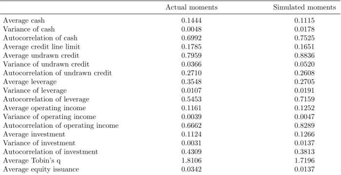
We now proceed to formally estimate the parameters of the model by means of a simulation-based estimator, namely the simulated method of moments (SMM). We start by describing our data in some more detail. We present then the estimation method and provide a discus-sion on identification. Finally, we present our results.
4.1.
Data
Estimating the dynamic corporate liquidity model requires merging data from different sources. In particular, we obtain financial statements data from Compustat annual files and credit lines data from Capital IQ. We remove all regulated (SIC 4900-4999) and financial firms (SIC 6000-6999). Observations with missing total assets, market value, gross capital stock, cash, long-term debt, debt in current liabilities, credit line limit, drawn portion of the credit line and SIC code are excluded from the final sample. We obtain a panel dataset with 19,796 observations for 3424 firms for the period of 2002 to 2011 at the annual frequency.
4.2.
Estimation
We estimate most of the model parameters using simulated method of moments (SMM). However, we estimate some of the model parameters separately. For example, we set the risk-free interest rate, r, equal the average over the sample period of the one-year Treasury rate. We set the depreciation of capital, δ, equal to 12%, which is the average depreciation rate in the Compustat dataset. Finally, we set the agency cost of holding cash, γ, equal to 0.77%, which corresponds to the estimate from DeAngelo, DeAngelo, and Whited (2011).
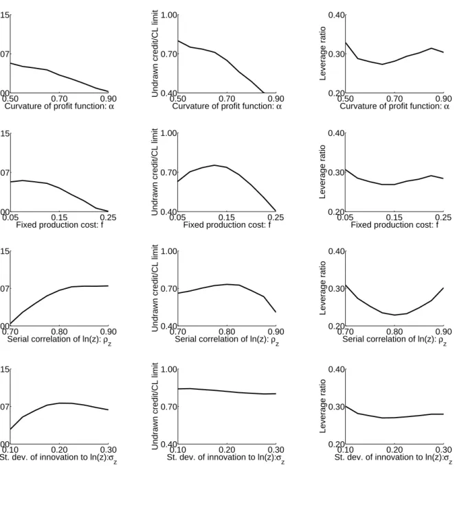
We then estimate 8 parameters using the simulated method of moments: the curvature of the profit function,α; the fixed production cost,f; the serial correlation ofln(z), ρz; the
standard deviation of the innovation of ln(z),σz; the fixed capital adjustment cost, ψ0; the