Munich Personal RePEc Archive
Banking Panic Risk and Macroeconomic
Uncertainty
Mikkelsen, Jakob and Poeschl, Johannes
Danmarks Nationalbank
27 June 2019
Online at
https://mpra.ub.uni-muenchen.de/98960/
Banking Panic Risk and Macroeconomic Uncertainty
∗
Jakob G. Mikkelsen
Johannes Poeschl
February 3, 2020
Abstract
We show that systemic risk in the banking sector breeds macroeconomic uncer-tainty. We develop a model of a production economy with a banking sector where financial constraints of banks can lead to disastrous banking panics. We find that a higher probability of a banking panic increases uncertainty in the aggregate economy. We explore the implications of this banking panic-driven uncertainty for business cy-cles, asset prices and macroprudential regulation. Banking panic-driven uncertainty amplifies business cycle volatility, increases risk premia on asset prices and yields a new benefit from countercyclical bank capital buffers.
Keywords: Banking Panics; Systemic Risk; Endogenous Uncertainty; Macropru-dential Policy
JEL Classification: E44; G12; G21; G28
∗Mikkelsen: Financial Stability Department, Danmarks Nationalbank, [email protected] and Poeschl: Research Department, Danmarks Nationalbank,[email protected]. Corresponding author: Johannes Poeschl. The authors thank Federico Ravenna, Luca Dedola, Raffaele Rossi, Kjetil Storesletten, Juan Rubio-Ram´ırez and seminar participants at Danmarks Nationalbank and the 2020 Meetings of the Danish Economic Society for comments. The viewpoints and conclusions stated are the responsibility of the individual contributors, and do not necessarily reflect the views of Danmarks Nationalbank.
1
Introduction
In this paper, we study how systemic risk in the banking sector affects the real economy through a novel feedback loop between systemic risk and macroeconomic uncertainty and explore how macroprudential policy can help to dampen this negative feedback loop.
The financial crisis of 2007-2009 was associated with a significant rise in both systemic risk in the banking sector and macroeconomic uncertainty more broadly: Fears of a systemic banking panic resulting in a disastrous breakdown of the financial sector were widespread. Measures of systemic risk in the banking sector increased substantially. In the first panel of Figure 1, we show the TED spread, which proxies the funding costs of the US banking sector and is thus a good indicator of systemic risk. The TED spread is usually close to zero, but increased almost tenfold from 0.38 in January 2007 to 2.45 in October 2008. This represented a substantial and unprecedented increase in systemic risk. At the same time, uncertainty in financial markets, which we proxy by the VIX in the second panel, increased dramatically to equally unprecedented levels.
This uncertainty spilled over into the aggregate economy: Measures of broader financial and macroeconomic uncertainty spiked, too. Consider for example the real uncertainty index constructed byJurado, Ludvigson, and Ng(2015). We show it in the third panel of Figure1. This index measures the conditional volatility in an exhaustive set of macroeconomic time series. During the financial crisis, it increased by about a third. As we show in the last three panels of Figure 1, credit risk premia spiked, and investment and output plummeted.
As a consequence of this disastrous event, the US and many other countries introduced a countercylical capital buffer (CCyB) for banks as a new policy instrument.1 One of the stated
purposes of such a policy is to reduce systemic risk in the economy by curbing excessive credit booms which can lead to severe downturns when they end.2 However, the exact
macroeconomic effects of this policy, in particular in a regime with elevated systemic risk, remain the subject of an ongoing debate.
These observations lead us to our research questions: How does an increase in systemic risk in the banking sector relate to an increase in macroeconomic uncertainty more broadly? What are the implications of endogenous systemic risk for business cycle dynamics and asset
1
See e.g. https://www.federalreserve.gov/newsevents/pressreleases/bcreg20160908b.htm for the US.
2
See e.g. Basel Committee on Banking Supervision (2010), page 7, paragraph 29: As witnessed during the financial crisis, losses incurred in the banking sector during a downturn preceded by a period of excess credit growth can be extremely large. Such losses can destabilise the banking sector, which can bring about or exacerbate a downturn in the real economy. This in turn can further destabilise the banking sector. These interlinkages highlight the particular importance of the banking sector building up its capital defences in periods when credit has grown to excessive levels. The building up of these defences should have the additional benefit of helping to moderate excess credit growth.
Figure 1: Measures of systemic risk (TED spread), aggregate uncertainty (VIX andJurado, Ludvigson, and Ng (2015)-Index), credit spreads, investment and real GDP.
Note: Sample period: 2006Q1 to 2013Q4. The TED spread is the month LIBOR minus the 3-month US treasury rate. The macroeconomic uncertainty index, which measures real uncertainty, is taken from Jurado, Ludvigson, and Ng (2015), available at https://www.sydneyludvigson.com/ data-and-appendixes. We use uncertainty at the 3-month horizon. The credit spread is the Moody’s BAA yield minus the federal funds rate. Real investment and output are detrended using the CBO potential output estimate.
prices? And how does the interaction between systemic risk and macroeconomic uncertainty affect the desirability of macroprudential policy?
To tackle these questions, we employ a simple, quantitative model of a production econ-omy with a financial sector. The key feature of the model is that disastrous banking panics can occur with an endogenous probability. It is based on the work by Gertler and Kiyotaki
(2015) and Gertler, Kiyotaki, and Prestipino (2019a): Households lend to banks, which in turn lend to firms. Firms use these loans to make investments. Due to a moral hazard problem in the spirit of Gertler and Karadi (2011), banks face an incentive constraint that limits their borrowing to a time-varying multiple of their equity. We interpret this incentive constraint as a market-imposed capital requirement. Crucially, the incentive constraint im-plies that a bank with zero or negative net worth cannot operate and must default. Together with the result that asset prices are increasing in bank net worth, the possibility of default implies that banks face systemic and self-fulfilling rollover crises in the spirit of Cole and Kehoe (2000) andGertler and Kiyotaki(2015). We followGertler, Kiyotaki, and Prestipino
(2019a) in calling these events banking panics. A banking panic of that kind occurs, when expectations about a banking panic drive down the values of banks’ assets so much that their net worth becomes negative. Banking panics are disastrous events, resulting in a large increase in credit spreads as well as a contraction of output, consumption and investment. We show that the dynamics of a banking panic in the model match the dynamics of asset prices and macroeconomic aggregates during the Great Recession in the United States well. Banking panics arise with an endogenous, time-varying probability. We define the probabil-ity of such a banking panic as systemic risk, using the terms banking panic risk and systemic risk interchangeably.
Our first main result is that an increase in systemic risk leads to an increase in macroe-conomic uncertainty, i.e. in the VIX and the conditional volatility of output. The model therefore provides a tight link between systemic risk in the financial sector and more broadly defined macroeconomic uncertainty. To our knowledge, making this link explicit and study-ing its implications in a dynamic stochastic general equilibrium model is a novel contribution to the literature. Systemic risk increases the conditional volatility of the economy, because the probability of a banking panic is endogenous and highly state-dependent. Since the probability of a banking panic in a state with a good realization of the exogenous shock is unchanged, output in those states is unaffected. In states of the world with a bad realiza-tion of the exogenous shock, the possibility of a banking panic increases the range of bad outcomes. Therefore, the presence of banking panic risk widens the conditional distribution of output by creating downside risk. Our results are consistent with the empirical results reported in Adrian, Boyarchenko, and Giannone (2019), who report that during times of
financial stress, the conditional distribution of GDP in the US has higher downside risk. Moreover, the empirical evidence in Giglio, Kelly, and Pruitt (2016) also provides strong support for the channel we emphasize by showing that an increase in systemic risk predicts a higher likelihood of a low realization of output.
For our second main result, we investigate the importance of this banking panic-driven uncertainty for macroeconomic dynamics. We find that banking panic-driven uncertainty is a novel channel that amplifies the response of the economy to a shock and increases the unconditional volatility of macroeconomic aggregates and asset prices. We arrive at this result by comparing an economy with endogenous banking panic risk to an economy without banking panics. Crucially, in the model without banking panics, banks otherwise face the same financial constraints as in our baseline model with banking panics. The transmission mechanism through which banking panic-driven uncertainty amplifies shocks works through a precautionary savings channel, a credit spread channel and a bank leverage channel: A negative macroeconomic shock increases the likelihood of a banking panic. Macroeconomic uncertainty about future consumption increases. As a consequence, the returns on risk-free assets fall as savers increase their demand for savings, seeking to insure themselves against future uncertainty. This is the precautionary savings channel. The returns on risky assets increase, as risk-averse investors demand higher risk premia. Higher risk premia in turn lead to a higher required return on investment for the non-financial sector and hence lower investment and output. This is the credit spread channel. Moreover, the moral hazard problem ties the borrowing capacity of banks to the market value of their net worth. As bank net worth is a risky asset, the return on banks’ net worth increases, implying that the market price of banks’ net worth falls. Banks are forced to contract lending, which increases the required return on investment for the non-financial sector. Output and investment fall. This is the bank leverage channel. Quantitatively, the bank leverage channel turns out to be the most important in our calibration, while the precautionary savings channel and the credit spread channel play a lesser role.
As our third main result, we investigate the importance of this novel banking panic uncertainty channel for macroprudential policy benefits. We focus on a dynamic capital requirement policy that the regulator sets to dampen credit booms, which lead to an excess build-up of systemic risk. In particular, we investigate the contributions of banking panics and systemic risk to the welfare effects of a policy that seeks to offset the feedback loop between asset prices, bank balance sheets and investment, i.e. the so called financial accel-erator effect (Bernanke, Gertler, and Gilchrist(1999)). Such a policy is desirable, because it enables the regulator to correct for the fact that banks fail to internalize that their lending decisions, through asset prices, affect the likelihood of a banking panic. There is therefore
a pecuniary externality in the model. Banking panics are inefficient, because they arise as a coordination of the agents on the dominated panic equilibrium. This equilibrium is domi-nated, because relative to the good no-panic equilibrium, lending to the non-financial sector is not undertaken by the most efficient lenders, i.e. the banks. When we again compare the two models with and without banking panic uncertainty, we find that there is a new benefit from this policy in the model with banking panic-driven uncertainty, since dampening the financial accelerator also reduces the likelihood of a banking panic, which lowers uncertainty. Put bluntly, we show that macroprudential policy is more beneficial in a regime with elevated systemic risk in the banking sector.
Literature Our model builds on recent work by Gertler and Kiyotaki(2015) andGertler, Kiyotaki, and Prestipino(2019a). Relative to these authors, we focus on the effects of bank-ing panic risk on macroeconomic uncertainty and highlight the importance of this uncertainty channel. The key difference between our model and theirs is that households have recursive
Epstein and Zin (1989) (EZ) preferences, which allows us to have both an intertemporal elasticity of substitution and a relative risk aversion of above 1.3 This is desirable for several
reasons: First, it allows us to match asset price moments. Second, an IES of above 1 gives rise to a household preference channel through which uncertainty has an effect on macroe-conomic quantities (Tallarini (2000), Gourio (2012) and Isor´e and Szczerbowicz (2017)). The interaction between this household preference channel and the uncertainty stemming from endogenous financial crises is a novel contribution of this paper. Our focus on the uncertainty channel is moreover similar to Navarro(2014), who does not model endogenous financial crises, however.
More generally, our paper is at the intersection of the literature on financial crises in macroeconomic models and the literature on the effects of uncertainty on business cycles. We contribute to this literature by highlighting the effect of uncertainty that results from the possibility of banking panics as a new channel through which financial crises can af-fect macroeconomic dynamics. We argue that the macroeconomic uncertainty caused by the spike in systemic risk is an important feedback channel that amplifies the severity of financial crises. There are now many macroeconomic models of financial crises: Our paper belongs to a strand of the literature that models financial crises as rollover crises in the spirit ofCalvo(1988) and Cole and Kehoe(2000), e.g. Gertler and Kiyotaki(2015),Gertler, Kiyotaki, and Prestipino(2016),Paul(2018), andGertler, Kiyotaki, and Prestipino(2019a). Relative to these papers, ours is the only one about a real production economy with fully
3
The use of EZ preferences to match asset prices is common in the macro-finance literature, see e.g. Van Binsbergen, Fern´andez-Villaverde, Koijen, and Rubio-Ram´ırez(2012) orRudebusch and Swanson (2012).
endogenous and anticipated banking panics. Other papers model financial crises as a finan-cial constraint of a leveraged agent becoming binding, e.g. Mendoza(2010),Bianchi(2011),
He and Krishnamurthy (2012), Brunnermeier and Sannikov(2014) andAkinci and Queralto
(2017).
Due to this focus on macroeconomic uncertainty, our paper also naturally connects to the macroeconomic literature on the effects of macroeconomic uncertainty on macroeconomic dynamics. Relative to the former literature, we first present banking panic risk as a novel channel through which macroeconomic uncertainty can arise endogenously. Second, we study how uncertainty feeds back into amplifying systemic risk. Third, we show that an increase in uncertainty due to banking panic risk is not symmetric, but concentrated in the left tail of the output distribution. In general, this literature focuses on exogenous, symmetric uncertainty shocks, e.g. Born and Pfeifer(2014),Fern´andez-Villaverde, Guerr´on-Quintana, Kuester, and Rubio-Ram´ırez (2015), Leduc and Liu (2016) and Basu and Bundick (2017). Others, e.g.
Fajgelbaum, Schaal, and Taschereau-Dumouchel (2017) or Cacciatore and Ravenna (2018) present mechanisms in which uncertainty arises endogenously or in which exogenous uncer-tainty shocks get endogenously amplified. The idea that small probabilities of large disasters can have big consequences for asset prices and macroeconomic dynamics has been explored, in a model with exogenous disasters, in Barro (2009) and Gourio (2012). Banking panics in our model can be interpreted as a particular kind of disaster that arises with an endoge-nous probability. Adrian, Boyarchenko, and Giannone (2019) and Alessandri and Mumtaz
(2019) present empirical evidence that financial stress and macroeconomic uncertainty are connected.
The paper is lastly related to the literature on the macroeconomic effects of bank regula-tion, in particular dynamic capital requirements. We study endogenous banking panic-driven uncertainty as a novel channel which affects the desirability of dynamic capital requirements. The macroeconomic effects of static capital requirements have been studied for example in
Angeloni and Faia (2013), Begenau and Landvoigt (2018) or Begenau (2019). Gertler, Kiy-otaki, and Queralto(2012) discuss dynamic capital requirements in a model with exogenous disasters. Faria-e Castro (2019) investigates the macroeconomic effects of countercyclical capital buffers on banking panics, but does not focus on the uncertainty channel. Gersbach and Rochet (2017) study countercyclical capital buffers in an economy in which pecuniary externalities lead banks to lend excessively, which causes misallocation.
Outline We proceed as follows: In section 2, we introduce the model, characterize the equilibrium and formalize banking panic risk. We calibrate the model in section 3. In section 4, we show what a typical banking panic in the model looks like. We explain how
banking panic risk affects macroeconomic uncertainty, and how macroeconomic uncertainty in turn feeds back into the economy in section 5. In section 6, we discuss macroprudential regulation. Finally, section 7concludes.
2
Model
The model is a production economy with a financial sector, based onGertler, Kiyotaki, and Prestipino (2019a). The key feature of the model is that financial frictions in the banking sector can lead to self-fulfilling rollover crises for banks in the spirit of Calvo (1988), Cole and Kehoe(2000) andGertler and Kiyotaki(2015). As we will show below, this implies that depending on the state of the economy, it can be in three different zones: A safe zone, where banking panics are not possible; a crisis zone, where a self-fulfilling rollover crisis is possible, and a default zone, where the banking sector will default with certainty.
The structure of the model is as follows: There are many households which each consist of a measure f of workers and a measure 1−f of bankers. Within each household, there is perfect consumption risk sharing. The households own and operate firms which produce consumption goods, firms which produce investment goods, and mutual funds. Workers supply a unit of labor in fixed supply, make loans to consumption goods producers and deposits to banks. Bankers own and operate banks. They use debt and their net worth to make loans to consumption goods producers. Banks accumulate retained earnings until they exit the economy with exogenous probability. In that case, they transfer the retained earnings as dividend income to their household. A moral hazard problem limits the ability of banks to issue debt to a time-varying multiple of their net worth, i.e. their leverage. Consumption goods producers own the capital stock, and use capital and labor to produce consumption goods. Investment goods producers transform consumption goods into investment goods using a technology which has decreasing returns to scale in the short run due to investment adjustment costs. Finally, mutual funds manage the portfolio of loans to consumption goods producers made directly by households against a fee. We begin by describing the non-standard part of the model, i.e. the household and banking sectors. We follow the convention that lower case letters for variables denote individual variables, while upper case letters denote aggregate variables.
2.1
Households
Preferences Households maximize utility from consumption. Their utility functionVH t is given by Epstein and Zin (1989) preferences, which are defined recursively as:
VtH = (1−β) cHt 1−σ +βhEt VtH+1 1−γi 1−σ 1−γ 1 1−σ , (2.1)
where Et denotes the expectation conditional on time t information and β is the discount factor of the household. cH
t denotes household consumption in period t. γ is the coefficient of relative risk aversion, σ the inverse of the intertemporal elasticity of substitution of the household. These preferences imply that the stochastic discount factor of the household is given by Λt,t+1=β cH t+1 cH t −σ VH t+1 h Et VtH+1 1−γi 1 1−γ σ−γ . (2.2)
With σ =γ, this preference specification collapses to constant relative risk aversion prefer-ences. γ > σ implies that households have a preference for early resolution of uncertainty.
Budget constraint Workers consume, make state-contingent long-term loans to consump-tion goods producers aH
t+1 through mutual funds and hold non-state-contingent one-period debt dH
t+1 issued by banks. They also have access to a risk-free one-period bond bHt+1, which is in zero net supply. We introduce this bond to ensure that the concept of a risk-free interest rate is well-defined.4 Since loans to consumption goods producers are effectively
claims on the capital stock of those firms, they are valued at the market price of capital Qt. The investments of workers into firms are managed by mutual funds, which charge a capital management fee ft. Workers supply one unit of labor inelastically and receive wages Wt as labor income.5 They receive profits Πt of firms and banks. Loans to banks yield a return
˜ RD
t+1 in the subsequent period. Loans to firms pay a returnRAt+1. The budget constraint of the household is given by
cH t + (Qt+ft)a H t+1+bHt+1+dHt+1 =RtAa H t + ˜R D t d H t +R B t b H t +Wt+ Πt. (2.3) 4
Bank debt carries some default risk.
5
To keep the model as simple as possible, we model labor supply as constant. Endogenizing the labor supply choice is straightforward and would not substantially affect the results.
2.2
Banks
2.2.1 Setup
Objective function Banks are operated by bankers. They maximize VtB =EtΛt,t+1(1−pt+1)
ηnBt+1+ (1−η)VtB+1
, (2.4)
where Λt,t+1 is the stochastic discount factor of households from period t to t+ 1, η is a probability that the bank exits the economy, pt is the probability that the bank defaults in period t and nB
t is the net worth of the bank at the beginning of period t.
Entry and exit As in Gertler and Karadi (2011), we assume that with probability η, a banker will be forced to give up his bank, sell its assets, repay its liabilities and pay the net worth to households. We introduce this assumption to ensure that banks will not outsave their borrowing constraints. To keep the mass of bankers constant, an equal mass of workers will start operating a bank with start-up funding nB,newt . This start-up funding is given by a fractionυ of the total assets traded in the economy: nB,newt =υAt. It is necessary to include some start-up funding for new banks, since banks with zero net worth cannot operate.
Net worth Banks issue debt dB
t+1. They make loans to consumption good producersaBt+1, who use these loans to purchase capital. Since there are no financial frictions between the firms and banks, these loans can be understood as direct claims on the capital stock of firms.6
In periodt, incumbent banks obtain a gross return on loans, RA
t aBt . They pay a returnRDt dBt to households on their debt. An incumbent bank’s net worth at the beginning of periodt is given by: nB t =R A ta B t −R D t d B t . (2.5)
Banks will optimally accumulate net worth until they exit the economy. Hence, equity at the end of the current period is equal to the banks’ net worth. Since we focus on the macroeconomic dynamics in the short run, we assume that banks cannot issue additional equity. It is a common assumption in the literature that equity issuance carries at least some cost for banks, see e.g. Akinci and Queralto (2017), Begenau (2019) or Corbae and D’Erasmo (2018). Hence, the equity of banks corresponds to their net worth.
6
This is obviously a modeling shortcut to make bank balance sheets responsive to current market prices. Another way to introduce state-contingency into bank balance sheets is through defaultable long-term debt, e.g. as inFerrante(2018).
Balance sheet The balance sheet constraint of banks states that assets QtaB
t+1 equal liabilities dB
t+1 plus equity nBt:
QtaBt+1 =dBt+1+nBt . (2.6)
We define the leverage of a bank φB
t as the value of its assets divided by the value of its equity: φBt ≡ QtaB t+1 nB t . (2.7)
Moral hazard problem To motivate the existence of a market-imposed capital require-ment, we introduce the following moral hazard problem: banks can divert a fraction of their assets after they have made their borrowing and lending decisions. In particular, a fraction ψ, 0< ψ <1 of their loans to firms can be diverted by the banker for personal consumption. If bankers divert assets, they will not repay their liabilities. Their creditors, i.e. the workers of other households, will force the banks to exit the economy if they observe diversion. The owner of the bank will return to being a worker. Because diversion occurs at the end of the period before next-period uncertainty realizes, an incentive constraint on the banks can ensure that diversion will never occur in equilibrium. This incentive constraint states that the benefit of diversion must be smaller or equal to the continuation value of the bank:
ψQtaBt+1 ≤VtB (2.8)
Dividing by net worth and defining ΩB
t ≡ VtB/nBt , we can see that 2.8 corresponds to a market-imposed leverage constraint:
φB t ≤ 1 ψΩ B t . (2.9)
Regulation The regulator follows a dynamic policy, which corresponds to a countercyclical capital buffer (CCyB). We model this policy as an upper bound on leverage. Similar to
Gertler, Kiyotaki, and Prestipino (2019b), we consider a dynamic rule where the regulator sets the capital buffer to react to the net worth of the banking sector. This is the state variable that is the most relevant to describe the state of the banking sector in the model. It co-moves strongly with variables that regulators use to determine the CCyB in reality, like
the credit-to-GDP gap. φBt ≤φ¯ B t , (2.10) ln ¯φB t = ln ¯φB−τ(lnNtB−lnNB). (2.11)
Forτ >0, this formulation implies that the regulator tightens the leverage constraint when-ever net worth of the aggregate banking sector NB
t is higher than its net worth in the stochastic steady stateNB, with elasticity τ. ln denotes the natural logarithm.
2.2.2 Rollover Decision of Banks’ Creditors
We show in the appendix that the franchise value of operating a bank which does not receive an exit shock in period t, VB
t , is linear in the net worth of the bank:
Proposition 2.1. The value function of the bank is linear in its net worth: VB
t = ΩBt nBt ,
where ΩB
t > 0 only depends on the aggregate state of the economy, but not on bank-specific
variables.
With this, we can show that the incentive constraint 2.8 of the bank implies a borrowing limit is linear in its net worth:
dBt+1 ≤ Φt 1−Φtn B t , (2.12) Φt= EtΛt,t+1(η+ (1−η)Ωt+1) RA t+1 Qt −ψ EtΛt,t+1(η+ (1−η)Ωt+1)RtD+1 .
This implies that creditors are not willing to lend to the bank, when the net worth of the bank is negative. Moreover, negative net worth means by definition that the bank cannot repay its liabilities and is insolvent. Therefore, when
RA t a B t ≤R D t d B t , (2.13)
the bank must default. The creditors of the bank, which are the workers of other households than the household the bank belongs to, will liquidate the assets of the bank.7 The recovery
rate on their debt is given by
xDt = RA taBt RD t dBt . (2.14) 7
This assumption ensures that bankers do not internalize the effect of their decisions on the recovery value of banks’ creditors in default.
2.2.3 Equilibrium multiplicity and banking panics
Since the net worth of incumbent banks is among the state variables which determine the capital price, and the capital price vice versa determines the net worth of banks, there is the possibility for multiple equilibra to coexist given the same fundamental state of the economy in the model:8 If bank creditors believe that the capital price is high, they will continue to
lend to the incumbent banks. The incumbent banks remains solvent and can lend to the nonfinancial sector, which justifies the high capital price. If bank creditors instead believe that the capital price is low, they will not lend to the incumbent banks. As a consequence, incumbent banks become insolvent and stop lending to the nonfinancial sector. Moreover, we assume, in line withGertler and Kiyotaki (2015), that new banks postpone entry in such a situation. The resulting lack of bank lending justifyies the low capital price.9
Define two recovery values for an individual bank: The recovery value xD
t denotes the recovery value of an insolvent, individual bank if there is no systemic banking panic. The recovery value xD∗
t denotes the recovery value of an individual bank if a systemic banking panic arises. Since the banks assets in the latter case are valued at fire-sale prices,xD
t > xD ∗ t . We can divide the state space of the model into three zones. In the first zone, the safe zone, both the recovery value without a systemic bank default, xD
t , as well as the recovery value of bank creditors with a systemic bank default, xD∗
t , are bigger than one. This implies that independent of the beliefs of bank creditors about the solvency of the banking sector, the banking sector is solvent. In that case, the no-panic equilibrium is the unique equilibrium of the economy.
In the second zone, the crisis zone, recovery values are bigger than one if the banking sector as a whole is solvent, but smaller than one if there is a systemic bank default. In this zone, both the equilibrium with solvent banks and the equilibrium with insolvent banks exist, because the solvency of banks depends on the beliefs of bank creditors about whether or not the banks are solvent. If agents coordinate on the equilibrium with insolvent banks, we follow Gertler, Kiyotaki, and Prestipino(2019a) in calling this a banking panic.
In the third zone, the default zone, both recovery valuesxD
t andxD ∗
t are less than one. As 8
As noted by Thaler (2018) and Christiano (2018), there is the possibility of a third, partial default equilibrium in the model, which turns out not to be quantitatively relevant for our calibration.
9
Note that in contrast to Diamond and Dybvig (1983), the decision of the bank creditors is not about whether to withdraw outstanding debt from the banks or not, but about whether they should roll over their lending to the banks or not. In that sense, a bank run in our model resembles more a rollover crisis in the spirit ofCole and Kehoe (2000) than to a depositor run as analyzed inDiamond and Dybvig (1983). The former corresponds more closely to the events of the financial crisis of 2007-2008, where financial institutions were unable to refinance maturing short-term liabilities on the interbank market. Strategic complementarity between the decisions of the bank creditors arises, because due to2.8, it is not optimal to lend to a bank with negative net worth.
in the crisis zone, both the panic and no-panic equilibrium exist, although there is a default of the incumbent banking sector in both equilibria in the default zone. The distinction between those equilibria in the default zone is that in the no panic equilibrium, new banks will continue to enter the economy, whereas in the panic equilibrium, they will postpone entry.10
We assume that if there are two equilibria, a sunspot shock Ξ will determine whether agents coordinate on the panic or the no-panic equilibrium. The sunspot shock can take on two values, ΞLand ΞH, with the probability of ΞH occurring given bypH. Agents coordinate on the panic equilibrium, if they observe the realization ΞH and on the no panic equilibrium otherwise.
The probability that the economy will end up in the banking panic equilibrium in the next period is then given by
pPanict+1 =pH❊ t ✶(xDt+1 ≤1 and xDt+1∗ ≤1) | {z } Default Zone +✶(xDt+1 >1 andx D∗ t+1 ≤1) | {z } Crisis Zone (2.15)
The probability of a default of the incumbent banking sector is equal to the probability of the economy experiencing a panic plus the probability of the economy being in the default zone without a panic occurring:
pDefaultt+1 =pPanict+1 + (1−p H )❊t ✶(xDt+1 ≤1 and x D∗ t+1 ≤1) (2.16) Note that the state-dependency of the banking panic probability arises only as a result of the state-dependency of the existence condition of the crisis zone and the default zone. There is no exogenous state-dependency built into the sunspot probability.
The return on deposits that households receive is given by ˜ RD t = ( min(xD t ,1)RDt if no panic occurs xD∗ t RDt if a panic occurs (2.17) 10
This corresponds to the way the equilibrium multiplicity is modelled inGertler, Kiyotaki, and Prestipino
2.2.4 Decomposing the banking panic condition
It will be useful to decompose the recovery value of bank creditors into four components: xD∗ t = RA,∗ t RA t | {z } 1−Liquidation discount RA t/Qt−1 RB t | {z } Firm credit spread RB t RD t |{z} Bank credit spread φt−1 φt−1−1 | {z } Bank leverage , (2.18) where RB
t is the risk-free interest rate. The first term is inversely related to the liquidation discount, which reflects how much asset returns fall in a banking panic. The second and third term measure the spread between the return on bank assets and the return on bank liabilities, which can be interpreted as bank profitability. The last term is inversely related to bank leverage. The model predicts that a banking panic is more likely if the expected liquidation discount is higher, the realized firm credit spread is lower, the bank credit spread is higher and bank leverage is higher.
2.3
Consumption goods producers
Consumption goods producers choose labor lF
t , capital sFt+1 and loans aFt+1 to maximize
❊t ∞ X s=t Λt,sΠFs. (2.19) Profits ΠF t are given by ΠFt = (k F t ) α (lFt )1 −α −WtlFt +Qt aFt+1− RA t Qta F t | {z } Borrowing −QtsFt+1−(1−δ)k F t | {z } Investment .
We make a distinction between beginning-of-period capital kF
t and end-of-period capitalsFt. Beginning-of-period capital is given by kF
t = ZtsFt . Following Merton (1973) and Gertler
and Karadi (2011), Zt is a capital quality shock which generates exogenous variation in the price of capital. We interpret it as fraction of the capital stock becoming obsolete and losing its economic value. The difference to depreciation δ is that the capital quality shock arises before production, whereas depreciation occurs after production. It follows an AR(1) process:
ln(Zt) = (1−ρZ)µZ+ρZln(Zt−1) +ǫt, (2.20) where |ρZ| < 1 and ǫt ∼ N(0, σZ). Since firms refinance themselves exclusively with loans from both banks and mutual funds, their balance sheet constraint is sF
optimality condition for bank loans implies that RAt =Zt α(k F t ) α−1 (lFt )1 −α + (1−δ)Qt. (2.21)
2.4
Capital goods producers
Capital goods producers transform consumption goods into capital goods with a technology that has decreasing returns to scale in the short run due to investment adjustment costs. They maximize profits ΠQt with respect to their output, it. Profits are given by
ΠQt =Qtit−it− θ 2 it It−1 −1 2 It−1. (2.22)
Note that capital producers take aggregate investment in the last period, It−1, as given.11 Hence, the problem of the capital producer is static.
2.5
Mutual funds
Competitive mutual funds manage the portfolio of loans that households directly invest into the consumption goods producers. FollowingGertler, Kiyotaki, and Prestipino(2019a), they face a cost function of providing this service, which is quadratic in the amount of loan services ˜
aM
t they manage. For simplicity, we assume that managing one unit of loans from households aH
t+1 requires one unit of loan services ˜aMt+1. For their services, mutual funds charge a fee ft which is determined in equilibrium. There is a cutoff ζ below which the funds can manage capital as efficiently as banks. They maximize profits, which are given by
ΠMt =ft˜a M t+1− χ 2max ˜ aM t+1 At+1 −ζ,0 2 At+1 (2.23)
We model this cost as a function of the share of capital managed by the funds and not as a function of the level to ensure that the mutual fund sector can scale with the economy in the long run. The cutoff ζ represents the share of investment projects above which the banking sector can better evaluate and monitor. If the mutual fund sector is forced to undertake a larger share of investment, e.g. due to the banking sector being insolvent, an efficiency loss arises.
11
Usually in the business cycle literature, firms internalize the effect of their investment decisions on future investment adjustment costs. Moreover, the investment adjustment cost is usually normalized with respect to It instead ofIt−1. Since the cost function under these two assumptions is very badly behaved for levels
of investment far away from the lagged level of investment, and since we solve for the global equilibrium dynamics of the model, we have adopted this simpler, better behaved formulation.
2.6
Aggregation
Since the policy functions of an individual bank are linear in net worth, we will characterize the equilibrium in terms of the aggregate banking sector. The aggregate net worth of the banking sector is given by the sum of the net worth of incumbent and newly entering banks:
NtB = (1−η)n B t +ηn
B,new
t .
Aggregate output is given by production net of the capital holding costs:
Yt =Ktα− χ 2 max ˜ AM t+1 At+1 −ζ,0 !2 At+1. (2.24)
We define as aggregate investment ˜Itas the total expenditure necessary to change the capital stock from Kt toSt+1. Therefore, our measure of aggregate investment includes the invest-ment adjustinvest-ment costs: Define It as net investment excluding capital adjustment costs, that is
It =St+1−(1−δ)Kt. Then, investment is given by
˜ It =It+ θ 2 It It−1 −δ 2 It−1. (2.25)
There is a representative household. Hence, the individual consumption and aggregate consumption are equal,cH
t =CtH. Household consumption can be inferred from the aggregate resource constraint:
CtH =Yt−It˜ (2.26)
2.7
Measuring uncertainty
2.7.1 Macroeconomic uncertainty
To formalize our notion of uncertainty, we rewrite future output Yt+1 as the sum of a fore-castable component EtYt+1 and an unforecastable component YtU+1:
The unforecastable component YU
t+1 depends on the distribution of future capital quality shocks ǫt+1, sunspot shocks Ξt+1 and the endogenous response of the economy to those shocks, e.g. due to a banking panic. Our measure of macroeconomic uncertainty is the volatility of the unforecastable component, which is equal to the conditional volatility of output:
StDevt(Yt+1) =StDevt(YtU+1) =
q
Et(Yt+1−EtYt+1)2 (2.28) Intuitively, this conditional volatility tells us how much uncertainty there is around the forecast for output in the next period. This definition of uncertainty is consistent with the one used in Jurado, Ludvigson, and Ng (2015).
2.7.2 Financial uncertainty
In addition to conditional output volatility, we include the VIX as a measure of uncertainty that is commonly used both in the academic literature and in policy discussions. We compute the VIX as V IXt = 100 s 4V art RA t+1 Qt , (2.29)
in line with Basu and Bundick (2017). We compute the conditional variance of the asset return in the same way as the conditional variance of output.
3
Calibration
We now turn to a quantitative evaluation of the macroeconomic effects of the banking panic-driven uncertainty channel. In this section, we outline the calibration strategy for the model and evaluate the model fit. The calibration is quarterly. We report the parameters in Table
1. We describe the data in Appendix A.
3.1
Calibration strategy
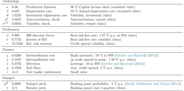
Technology We calibrate the parameter of the production function,α, to match a capital income share of 36 percent. We set the depreciation rateδ to match an annual depreciation rate of 10 percent. To calibrate the autocorrelationρZ and the standard deviationσZ of the capital quality process, we target the autocorrelation and standard deviation of output. We calibrate the investment adjustment cost parameter θ to target the volatility of investment.
Technology
α 0.36 Production function 36 % Capital income share (standard value)
δ 0.025 Depreciation rate 10 % Annual depreciation rate (standard value)
θ 1.0233 Investment adjustment cost Volatility, investment (data)
ρZ 0.8637 Autocorrelation, shock Autocorrelation, output (data) σε,Z 0.0044 Volatility, shock Volatility, output (data)
Preferences
β 0.995 HH discount factor Real risk-free rate: 1.87 % p.a. in SSS (data)
σ 0.7716 Inverse of IES Real risk-free rate volatility (data)
γ 10.5328 Rel. risk aversion Credit spread volatility (data) Finance
χ 0.0266 Intermediation cost Bank intermed.: 50 % in SSS (Gertler and Kiyotaki(2015))
ζ 0.1827 Intermediation cost ∆ credit spread in panic: 7.29 % p.a. (data)
ψ 0.3792 Diversion Leverage: 10 in SSS (Gertler and Kiyotaki(2015))
η 0.1093 Exit Rate Avg. credit spread: 3 % p.a. (data)
υ 1e-3 New banks’ endowment Small value
Sunspot
pH 0.0965 Sunspot prob. Banking panic probability: 4 % p.a. (Jord`a, Schularick, and Taylor(2011))
π 2/3 Reentry prob. Banking panics last 3 quarters (data)
Table 1: Calibration
Preferences We choose the preference parameters β, σ and γ to match asset prices. We set the discount factor of the household, β, to match the real risk-free interest rate in the stochastic steady state. To exclude the zero lower bound period, we use the average interest rate between the first quarter of 1986 to the last quarter of 2006 as the empirical counterpart. We choose the inverse of the intertemporal elasticity of substitution,σ, to match the volatility of the real risk-free interest rate and the risk aversion, γ, to match the volatility of the credit spread.
Financial sector There are five parameters for the financial sector: The loan management fee parameters χ and ζ, the share of divertable assets ψ, the exit rate of bankers η and the initial endowment of new bankers υ. We set these parameters jointly to target the following moments: A share of intermediation through the banking sector of 50 percent in the stochastic steady state, in line with Gertler and Kiyotaki (2015), a leverage of 10 in the stochastic steady state, in line with Gertler and Kiyotaki (2015), Begenau and Landvoigt
(2018) and the evidence in Di Tella (2019), a credit spread of about 3.7 percent in the stochastic steady state, consistent with the average spread between the Moody’s BAA yield and the Federal Funds Rate between the first quarter of 1986 and the last quarter of 2006 and an increase in the credit spread in a panic of 7.29 percent. This corresponds to the peak to trough change in the Moody’s BAA spread over the federal funds rate from the first quarter of 2007 to the fourth quarter of 2008.
Sunspot We set the sunspot probabilitypH to match a frequency of banking crises of about 4 percent per year, consistent with the frequency of financial crises in developed economies in
Jord`a, Schularick, and Taylor(2011). Finally, we set the persistence of the panic equilibrium π to target an average duration of a banking crisis of 3 quarters, which corresponds to the time until the TED spread returned to normal levels and the XLF financial equity index stopped falling after the banking panic in the last quarter of 2008.
3.2
Model Fit
Data Model
St. Dev., Output (%) 4.073 4.875
St. Dev., Investment (%) 12.311 10.090
Autocorrelation, Output 99.008 98.930
Deposit Rate in SSS (% p.a.) 1.870 1.875
Credit Spread in SSS (% p.a.) 3.886 3.885
St. Dev., Deposit Rate (%) 2.107 1.692
St. Dev., Credit Spread (%) 1.614 1.293
Bank Lending/Total Lending in SSS (%) 50.000 47.894
Bank Leverage in SSS 10.000 9.512
Bank Run Frequency (% p.a.) 4.089 4.156
Bank Run Duration (yrs) 0.750 0.747
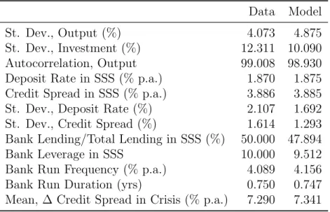
Mean, ∆ Credit Spread in Crisis (% p.a.) 7.290 7.341 Table 2: Targeted moments
Note: The simulated moments come from a simulation of 10000 economies for 2000 periods, discarding the first 1000 periods as burn-in. The stochastic steady state is computed as the state of the economy after a simulation of 1000 periods without any shocks.
Table 2reports how well the model fits the targeted moments. The standard deviation of output and investment are matched reasonably well. The model can match the autocorrela-tion of output. It also does a good job at matching asset prices with reasonable parameters for household preferences: the deposit rate and the credit spread in the stochastic steady state are matched well. The standard deviation of the deposit rate and the standard devia-tion of the credit spread are matched well. The model can match the ratio of bank lending to total lending and bank leverage. The frequency of banking panics is also matched well. Interestingly, we found in numerical exercises thatincreasing the sunspot probabilityreduces the frequency of banking panics. This is because an increase in the expected probability of a banking crisis forces banks to delever. This result is reminiscent of the volatility paradox discussed in Brunnermeier and Sannikov (2014). The banking panic duration and the in-crease in the credit spread during a banking panic are matched well. Overall, the model can
match all moments quite well, which is not trivial, given that it is a highly nonlinear model with complex dynamics.
4
A typical banking panic
After having calibrated the model, we first use it to study what a typical realized banking panic looks like. The purpose of this exercise is to ensure that banking panics in the model capture some stylized facts about financial crises in the data: Namely that they are disastrous events which cause a long-lived fall in macroeconomic aggregates and asset prices.
4.1
Peak-to-trough changes during the financial crisis of
2007-2009 in the model and in the data
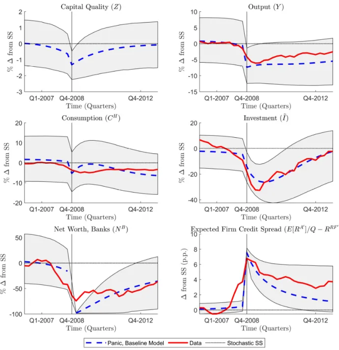
In Figure 2 and Table 3, we report the ability of the model to fit data from the financial crisis in the US during the period of 2007-2009. For this exercise, we compare the effect of a typical banking panic in the model on macroeconomic aggregates and asset prices to the peak-to-trough changes in those variables in the data.12 In line with Gertler, Kiyotaki, and Prestipino(2019a), we assume that a banking panic happened in the data in the last quarter of 2008. The last quarter of 2008 was when Lehmann Brothers failed, which was followed by major disruptions of financial markets and subsequent failures of other financial institutions. Consider first Figure 2. It shows the dynamics of key macroeconomic and financial variables around a typical banking panic in a simulation of the model.13 The blue, solid
line reports the average path of the respective variable around a typical panic. Since there is substantial heterogeneity in the paths, we also report the range in which 90 percent of all banking panics fall as the shaded area. The red line is the data. We can see that the model reproduces the dynamics of key macroeconomic aggregates and asset prices well. Note that we neither select the shocks to match a specific time series nor target any of the macroeconomic dynamics besides the credit spread in our calibration.
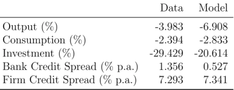
Consider next Table3. Consistent with the NBER recession dates for the financial crisis, we compute the change in output, consumption, and investment from the last quarter of 2007 to the second quarter of 2009. We compute the change in asset prices from the first
12
To construct the tables and figures in this section, we follow Paul (2018): first, we simulate 10000 economies for 1000 periods. We then find all banking panics and compute the average path around a typical panic event. We discard all panics where another panic happens within 100 quarters before to 20 quarters after the panic to ensure that we capture only the effect of a single panic.
13
This event study approach is different from showing the response to a specific series of shocks out of steady state.
Figure 2: Dynamics around a typical banking panic in the model and in the data. Note: The blue line denotes the response of an average economy around a banking panic. Since there is substantial heterogeneity in the simulation, the shaded area reports the range within which 90 percent of the typical banking crises fall. Moments of a simulation of 10000 economies for 1000 periods. We drop all crises where a previous crisis occurred in the last 100 quarters before the panic until 20 periods after the panic. The data for output, consumption and investment are detrended using the CBO potential output estimate. The credit spread is the spread between the Moody’s BAA yield and the Federal Funds Rate. The financial sector net worth is the XLF index as a percentage deviation from the 2007Q3 value.
quarter of 2007 to the last quarter of 2008, since the stress in the financial markets started earlier and peaked in the last quarter of 2008, simultaneously with the banking panic.
Data Model
Output (%) -3.983 -6.908
Consumption (%) -2.394 -2.833
Investment (%) -29.429 -20.614
Bank Credit Spread (% p.a.) 1.356 0.527 Firm Credit Spread (% p.a.) 7.293 7.341
Table 3: Peak-to-trough changes during the financial crisis of 2007-2009 in macroeconomic aggregates and asset prices in the model and the data.
Note: For output, consumption and investment, we define the peak of the great recession as the last quarter of 2007 and the trough as the second quarter of 2009, consistent with the NBER recession dates. For the bank credit spread and the firm credit spread, we define the peak as January 2007 and the trough as October 2008. The model moments come from a simulation of 10000 economies for 2000 periods, discarding the first 1000 periods as burn-in.
The model does a good job at matching a fall in output of a roughly similar magnitude as in the data. The model produces a similar fall in consumption around a typical banking panic compared to the financial crisis in the US. The fall in the model is a bit larger, because it is more persistent than in the data. The fall in investment in the model is smaller than in the data. The rise in bank credit spreads is too small. This is natural, the model lumps together all bank liabilities, which includes not only market lending, which is our data counterpart, but also bank deposits. The model also matches the increase in the cost of financing to the real economy.
4.2
Model dynamics around a typical banking panic
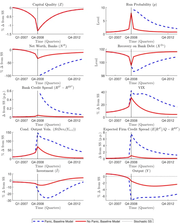
After comparing the model to the data, we now focus on the mechanism of how a banking panic unfolds in the model. Figure 3 shows the dynamics of additional variables around a banking panic. The blue line is the path if a banking panic occurs. The red line is the counterfactual average path if there is no panic in period zero. The difference between the blue line and the red line gives us the additional impact of an average banking panic, given the same initial conditions and the same sequence of capital quality shocks.14 The thin,
black line reports the value of the respective variable in the stochastic steady state.
In the first panel, we show the sequence of exogenous capital quality shocks around a typical banking panic. These shocks are of course identical for the panic and the no panic economies. We observe that banking panics typically arise after a sequence of negative
14
Alternatively, it gives us the additional change in the variable from moving from the equilibrium with solvent banks to the equilibrium with a systemic bank default.
Q1-2007 Q4-2008 Q4-2012 -1.5 -1 -0.5 0 Q1-2007 Q4-2008 Q4-2012 0 5 10 Q1-2007 Q4-2008 Q4-2012 -100 -50 0 Q1-2007 Q4-2008 Q4-2012 98 100 102 Q1-2007 Q4-2008 Q4-2012 0 0.2 0.4 0.6 Q1-2007 Q4-2008 Q4-2012 0 20 40 Q1-2007 Q4-2008 Q4-2012 0 50 100 150 Q1-2007 Q4-2008 Q4-2012 0 2 4 6 8 Q1-2007 Q4-2008 Q4-2012 -30 -20 -10 0 10 Q1-2007 Q4-2008 Q4-2012 -6 -4 -2 0
Panic, Baseline Model No Panic, Baseline Model Stochastic SS
Figure 3: Dynamics around a typical banking panic - exploring the mechanism. Note: The blue line denotes the response of an average economy around a banking panic. The red line shows the average path, across economies, if no banking panic occurs, given the same initial conditions and the same sequence of shocks. Moments of a simulation of 10000 economies for 1000 periods. We drop all crises where a previous crisis occurred in the last 100 quarters before the panic until 20 periods after the panic.
capital quality shocks. The shocks reduce the net worth of banks and the recovery value in the case of a banking panic. As a consequence, the likelihood of a banking panic increases. Due to the higher likelihood of a panic, financial uncertainty, as measured by the VIX, and macroeconomic uncertainty, as measured by the conditional output volatility, increase.
If a panic is triggered, bank net worth and bank lending fall to zero and financial inter-mediation will only occur through the mutual fund sector. It is best to think of the mutual fund sector in our model as the part of the financial sector in which financial frictions played a lesser role during the financial crisis, like smaller commercial banks. The banking sector in our model should be interpreted as comprising large commercial banks and shadow banks, including broker-dealers. This fall in bank intermediation leads to a spike in the expected firm credit spread, as mutual funds require a higher expected return than banks. As a con-sequence, we see that investment decreases dramatically, and so does output due to both the lower capital stock and the efficiency losses due to the lack of bank intermediation.
After the banking panic, the net worth of the banking sector slowly rebuilds as new banks start to enter the economy. Expected returns on firm loans are high, due to the high required return of mutual funds. Newly entering banks are therefore highly profitable, which also means that they have a high leverage capacity. High bank leverage in turn lowers expected recovery values, which increases the likelihood of a second banking panic in the aftermath of the first one. Hence, credit spreads and conditional volatility remain elevated and investment and output subdued until the net worth of the banking sector has fully rebuild.
Overall, we can see that banking panics are dramatic events which substantially influence the dynamics of both macroeconomic aggregates and asset prices. Moreover, we can see that banking panic risk is reflected in asset prices even before the panic occurs. A particular strength of the model is that it produces the empirically observed co-movement in asset prices and quantities before and after banking panics.
5
Banking panic risk and macroeconomic uncertainty
In the last section, we have studied the conditional response of the economy to a realized banking crisis. We have shown that both the build-up and the aftermath of a banking crisis are episodes of high systemic risk and high conditional volatility. While banking crises are dramatic events, they are however also rare events, such that it is unclear whether systemic risk in the financial sector should have an effect on aggregate uncertainty and macroeconomic dynamics outside a banking panic. In this section, we illustrate how an increase in banking panic risk can increase macroeconomic uncertainty. We show that both
banking panic risk and macroeconomic uncertainty are highly state-dependent. Finally, we discuss how macroeconomic uncertainty affects the economy and feeds back into banking panic risk through a precautionary savings channel and a financial frictions channel.
5.1
The effect of banking panic risk on macroeconomic
uncer-tainty
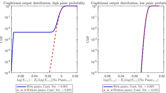
To illustrate the effects of banking panic risk on conditional output volatility, we consider the following thought experiment: Suppose we compare two economies which are identical, economy A and economy B. The only difference is that in economy A, sunspot shocks can lead agents to coordinate on the panic equilibrium if multiple equilibria are possible, whereas in economy B, agents never coordinate on the panic equilibrium if multiple equilibria are possible. By how much is the conditional volatility of output in economy A in the region with equilibrium multiplicity higher than in economy B?
-0.06 -0.04 -0.02 0 0.02 10-6 10-5 10-4 10-3 10-2 10-1 100 -0.06 -0.04 -0.02 0 0.02 10-6 10-5 10-4 10-3 10-2 10-1 100
Figure 4: The conditional distribution of output in economies with and without panics. Note: We hold the state of the economy at timet fixed. The policy functions come from the numerical solution of the model under the baseline calibration, where for the economy with sunspots,pH
= 0.1 while for the economy without sunspots,pH
= 0.
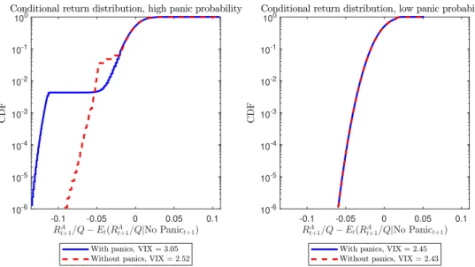
The left panels of Figures 4 and 5 show the cumulative distribution function of the conditional distribution of output and asset returns. The economy with panics is the solid blue line and the economy without panics the dashed red line. We compare the economies for the same state of the economy at time t. We can see that for the economy without panics, the range of possible realizations of output is distributed symmetrically around expected output. In contrast to that, for the economy with panics, a second, albeit small fraction of the distribution lies at around 7 percent below expected output. As a consequence of
-0.1 -0.05 0 0.05 0.1 10-6 10-5 10-4 10-3 10-2 10-1 100 -0.1 -0.05 0 0.05 0.1 10-6 10-5 10-4 10-3 10-2 10-1 100
Figure 5: The conditional distribution of asset returns in economies with and without panics. Note: We hold the state of the economy at timet fixed. The policy functions come from the numerical solution of the model under the baseline calibration, where for the economy with sunspots,pH= 0.1 while for the economy without sunspots,pH = 0.
this, the conditional volatility of output is roughly twice as high in the economy with panics compared to the economy without panics.
This increase in the conditional volatility of output and asset returns will only arise in future states of the economy where the banking panic equilibrium exists, which depends on the state of the economy today. As a consequence, the conditional volatility of output and asset returns are endogenously highly state-dependent. To illustrate this, consider the right panels of Figures 4and 5. These compare the economy with panics to the economy without panics in a state in which there is no banking panic risk. In this state, the conditional volatility of future output and asset returns are essentially identical in both economies. Banking panic risk thus only increases the left tail of the output distribution, and only during times of heightened financial stress, in line with the empirical evidence in Giglio, Kelly, and Pruitt (2016) and Adrian, Boyarchenko, and Giannone (2019).
5.2
Banking panic risk as an amplification mechanism
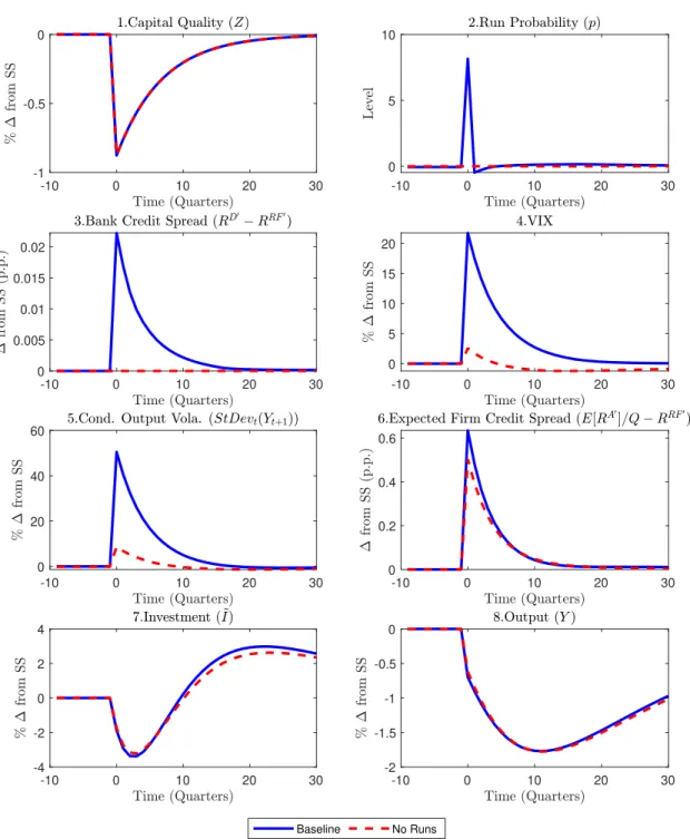
In Figure 6, we show the generalized impulse response of the economy to a two standard deviation negative capital quality shock, conditional on no panic occurring. The blue lines are the impulse responses from the baseline model in which banking panics can occur, the red lines are those from an alternative model without banking panics.
We see that the shock increases the probability of a banking panic in the baseline model. As a consequence, macroeconomic and financial uncertainty increase. In the model without
-10 0 10 20 30 -1 -0.5 0 -10 0 10 20 30 0 5 10 -10 0 10 20 30 0 0.005 0.01 0.015 0.02 -10 0 10 20 30 0 5 10 15 20 -10 0 10 20 30 0 20 40 60 -10 0 10 20 30 0 0.2 0.4 0.6 -10 0 10 20 30 -4 -2 0 2 4 -10 0 10 20 30 -2 -1.5 -1 -0.5 0 Baseline No Runs
Figure 6: The impulse response to a two-standard deviation negative capital quality shock. Note: Impulse response to two-standard deviation capital quality shock. Baseline is the model with banking panics. No Runs is a model in which we set the sunspot probability to zero.
banking panics, this increase is substantially lower. Credit spreads for both banks and firms increase more in the baseline model. Taken together, these results show that the possibility of banking panics has a strong effect on uncertainty and asset prices. Regarding quantities, both the initial fall and the recovery of investment and output are amplified in the model with panics. This is because the higher credit spread allows banks to accumulate net worth faster.
5.3
The feedback loop between banking panic risk and
macroeco-nomic uncertainty
The increase in macroeconomic uncertainty due to the higher banking panic risk affects the macroeconomy through three channels:
First, a precautionary savings channel, working through the risk-free interest rate, leads households to reduce their demand for bank debt and their demand for loans issued by the non-financial sector: Consider first the households’ first-order condition for the risk-free bond:
1 = ❊tΛt,t+1RBt+1. (5.1)
Using the definition of the stochastic discount factor, we can write the risk-free interest rate as RBt+1 = ❊tβ CH t+1 CH t −σ | {z } CRRA VH t+1 h Et VtH+1 1−γi 1 1−γ σ−γ | {z } LRR −1 . (5.2)
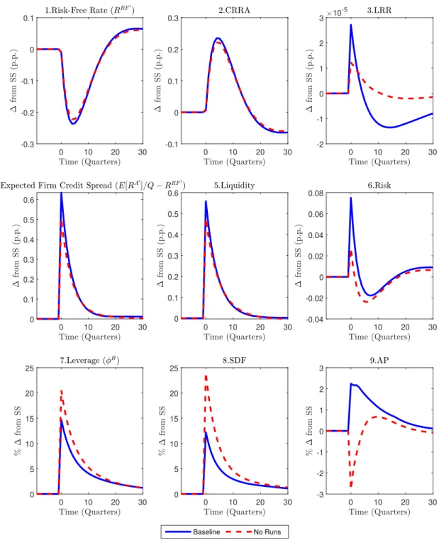
The first term, CRRA, corresponds to the stochastic discount factor with constant relative risk aversion and is concave in consumption growth in the next period. The second term, LRR, is concave in long-run consumption growth, ifγ > σ. The first three panels of Figure
7 show the generalized impulse response of the risk-free interest rate as well as its two components, CRRA and LRR, after a two standard-deviation negative capital quality shock. We can see that there is a small additional fall in the risk-free interest rate in the model with panics compared to the model without panics, mostly due to the CRRA term. The model does not generate a big amount of long-run risk, such that the contribution of the LRR term to the fall in the risk-free rate is small.
0 10 20 30 -0.3 -0.2 -0.1 0 0.1 0 10 20 30 -0.1 0 0.1 0.2 0.3 0 10 20 30 -2 -1 0 1 2 3 10 -5 0 10 20 30 0 0.1 0.2 0.3 0.4 0.5 0.6 0 10 20 30 0 0.1 0.2 0.3 0.4 0.5 0.6 0 10 20 30 -0.04 -0.02 0 0.02 0.04 0.06 0.08 0 10 20 30 0 5 10 15 20 25 0 10 20 30 0 5 10 15 20 25 0 10 20 30 -3 -2 -1 0 1 2 3 Baseline No Runs
Figure 7: The effects of uncertainty - exploring the mechanism.
Note: Impulse response to two-standard deviation capital quality shock. No Runsis a model in which we set the sunspot probability to zero.
Consider next the first-order condition for the direct lending of the household to the non-financial sector:
Qt+ft=❊tΛt,t+1RAt+1. (5.3)
Using this equation, we can write the credit spread as
❊t RA t+1 Qt −R B t+1 = ft Qt |{z} Liquidity −covt RA t+1 Qt ,Λt,t+1 | {z } Risk RBt+1
There are two important terms. The first, ft
Qt, reflects a liquidity premium that is higher
when households hold a larger share of the assets of the economy. The second term reflects a risk premium for the correlation between the stochastic discount factor and the return on loans. Panels 4 to 6 of Figure7show the generalized impulse responses of the credit spread, as well as the liquidity premium and the risk premium. The credit spread increases more in the model with banking panics. As we can see, a large fraction of the increase in the credit spread stems from the liquidity premium, which reflects financial constraints of banks and is similar in both models. The additional increase in the credit spread we see in the model with panics stems however mostly from the risk premium, which increases substantially more in the model with panics.
Finally, an increase in uncertainty operates through a bank leverage channel, which tightens the leverage constraint of banks 2.8. This leverage constraint can be rewritten as
φB t =EtΩ˜Bt+1 | {z } SDF RD t+1 ψ−EtΩ˜Bt+1 RA t+1 Qt −R D t+1 | {z } AP (5.4) ˜ ΩB t+1 = Λt,t+1(1−pt+1) η+ (1−η)ΩB t+1
There are two key terms: First, the adjusted stochastic discount factor of the banking sector, SDF, which reflects the value of an additional unit of net worth in the banking sector in the next period from the perspective of the households owning the banks. Second, there is a term, AP, which relates to asset prices. It is increasing in both the deposit rate and the credit spread. The last three panels of Figure 7 show the impulse responses of leverage, as well as the stochastic discount factor and the asset price term. Leverage increases less in the model with banking panics, reflecting relatively tighter financial constraints. We can
see that most of the change in leverage comes from the stochastic discount factor, which reflects that if there is default risk in the banking sector, the value of an additional unit of net worth in the banking sector is lower. The term related to asset prices actually increases more, reflecting the higher credit spread in the model with panics, but it is ultimately less important for leverage dynamics.
Taken together, we can see that the quantitatively most important channel through which panic risk affects the economy is the bank leverage channel, with the credit spread channel playing a somewhat smaller role, and the precautionary savings channel being unimportant.
5.4
The role of EZ preferences
Figure 8 illustrates the crucial role of EZ preferences for the effects of uncertainty being in line with the effects of uncertainty shocks in the empirical literature; namely, a fall in output and investment and a rise in credit spreads in response to an increase in uncertainty.15 The
figure shows the difference in the impulse response to a two standard deviation negative capital quality shock between an economy with banking panics and an economy without banking panics. This corresponds to the difference between the blue and the red line in Figure 6. Intuitively, this is the additional impact of the capital quality shock due to the increase in endogenous banking panic risk. The blue line is the response of the baseline model with EZ preferences, the red line the response of an alternative model with constant relative risk aversion (CRRA) preferences, withγ =σ = 2.
We can see that the impact of the capital quality shock on the probability of a banking panic is similar in both models. The economy with EZ preferences experiences a larger increase in bank credit spreads and conditional output volatility, while the response of the VIX is similar. The important distinction is in terms of the firm credit spread, where the additional uncertainty due to banking panic risk leads to a fall in the credit spread in the model with CRRA preferences, and to a rise in the model with EZ preferences. Heightened uncertainty also leads to a rise in investment and output in the model with CRRA preferences, whereas it leads to a fall in investment and output in the model with EZ preferences.
Figure 9 revisits the decomposition of the effects of uncertainty of Figure 7. As in Figure8, we show the difference in impulse responses between economies with panic risk and economies without panic risk for two different preference specifications. We can see that due
15
See e.g. Jurado, Ludvigson, and Ng(2015) orAlessandri and Mumtaz(2019). The literature studies the effects of uncertainty shocks, whereas we study the effects of the presence of endogenous uncertainty. While the mapping between their results and ours is not perfect, the effects of an uncertainty shock still should be informative for the effects of endogenous uncertainty.
-10 0 10 20 30 -1 -0.5 0 0.5 1 -10 0 10 20 30 0 5 10 -10 0 10 20 30 0 0.005 0.01 0.015 0.02 -10 0 10 20 30 0 5 10 15 20 -10 0 10 20 30 0 10 20 30 40 -10 0 10 20 30 -0.1 -0.05 0 0.05 0.1 -10 0 10 20 30 -0.5 0 0.5 1 -10 0 10 20 30 -0.1 0 0.1 0.2 Baseline CRRA
Figure 8: Amplification of a first moment capital quality shock due to endogenous uncertainty - the role of preferences.
Note: Impulse responses with banking panics minus impulse responses without banking panics. Baseline
0 10 20 30 -0.2 -0.15 -0.1 -0.05 0 0.05 0 10 20 30 -0.05 0 0.05 0.1 0.15 0.2 0 10 20 30 -1.5 -1 -0.5 0 0.5 1 1.5 10 -5 0 10 20 30 -0.15 -0.1 -0.05 0 0.05 0.1 0.15 0 10 20 30 -0.15 -0.1 -0.05 0 0.05 0.1 0 10 20 30 -0.02 0 0.02 0.04 0.06 0 10 20 30 -8 -6 -4 -2 0 2 0 10 20 30 -15 -10 -5 0 0 10 20 30 -6 -4 -2 0 2 4 6 Baseline CRRA
Figure 9: Amplification of a first moment capital quality shock due to endogenous uncertainty - decomposition.
Note: Impulse responses with banking panics minus impulse responses without banking panics. Baseline
to the lower IES in the model with CRRA preferences, the additional impact of uncertainty leads to a much stronger fall in the risk-free rate compared to the model with EZ preferences. The fall in the credit spread in the model with CRRA preferences is mostly driven by a fall in the liquidity premium, as households’ capital holdings increase relatively less. Finally, whereas the effects of household preferences are very different in the two models, the fall in leverage is similar. However, whereas it is driven by two offsetting effects due to higher credit spreads and a lower stochastic discount factor in the model with EZ preferences, the effect on leverage in the model with CRRA preferences mostly stems from the fall in the risk-free interest rate.
Overall, we see that EZ preferences are crucial to achieve effects of heightened uncertainty that are in line with the empirical literature, namely an increase in credit spreads and a fall in investment and output.
5.5
Unconditional effects of banking panic risk
We study next the unconditional effects of banking panic risk on macroeconomic uncer-tainty and business cycle dynamics. We first show that elevated banking panic risk increases macroeconomic uncertainty unconditionally. Second, we show that this time-varying uncer-tainty amplifies the volatility of macroeconomic aggregates and asset prices.
Table 4 shows that banking panic driven uncertainty amplifies macroeconomic volatil-ity. We compare and simulate two models: In the first model, panics are anticipated and materialize. In the second model, crises are unanticipated and never materialize.
We see that banking panic risk varies substantially over time: The unconditional proba-bility of a banking panic is about 4 percent per year. The probaproba-bility of a panic is moreover countercyclical, since bank leverage is high and realized bank asset returns are low during recessions, leading to low recovery values for bank creditors and hence elevated banking panic risk.
Banking panic risk increases aggregate uncertainty substantially. Output volatility in the model with banking panics is about 0.7 percent, in the model without banking panics, it is about 0.3 percent. The VIX in the model with banking panics is around 3.3 on average, in the model without banking panics, it is around 2.7.16 Both are also countercyclical, and the
countercyclicality is more pronounced in the model with banking panic risk.
Comparing the unconditional realized volatilities of output, consumption and investment of the models with and without banking panics in Table4, we see that banking panics increase
16
Note that we compute the VIX assuming that firms have zero leverage, and that we abstract from idiosyncratic risks. Taking those factors into account would allow us to also match the level of the VIX without changing the key results of the model.