Risk and Reciprocity Over the Mobile Phone Network: Evidence from Rwanda

NET Institute*

Working Paper #11-25

October 2011

Risk and Reciprocity Over the Mobile Phone Network: Evidence from Rwanda

Joshua Blumenstock

Nathan Eagle

Marcel Fafchamps

University of California, Berkeley Santa Fe Institute

Oxford University

* The Networks, Electronic Commerce, and Telecommunications (“NET”)

Institute

network industries, electronic commerce, telecommunications, the Internet, “virtual

networks” comprised of computers that share the same technical standard or operating

system, and on network issues in general.

Risk and Reciprocity Over the Mobile Phone Network: Evidence

from Rwanda

∗

Joshua Blumenstock

University of California, Berkeley

Nathan Eagle

Marcel Fafchamps

DRAFT VERSION

September 30, 2011

A large literature describes how local risk sharing networks can help individuals smooth consumption in the face of idiosyncratic economic shocks. However, when an entire community faces a large covariate shock, and when the transaction costs of transfers are high, these risk sharing networks are likely to be less effective. In this paper, we document how a new technology – mobile phones – reduces transaction costs and enables Rwandans to share risk quickly over long distances. We examine a comprehensive database of person-to-person transfers of mobile airtime and find that individuals send this rudimentary form of “mobile money” to friends and family affected by natural disasters. Using the Lake Kivu earthquake of 2008 to identify the effect of a large covariate shock on interpersonal transfers, we estimate that a current-day earthquake would result in the transfer of between $22,000 and $30,000 to individuals living near the epicenter. We further show that the pattern of transfers is most consistent with a model of reciprocal risk sharing, where transfers are determined by past reciprocity and geographical proximity, rather than one of pure charity or altruism, in which transfers would be expected to be increasing in the wealth of the sender and decreasing in the wealth of the recipient.

JEL Classification: O16, O17, O33

Keywords: Risk Sharing; Mobile Phones; Mobile Money; Information and communications tech-nologies; Development; Earthquakes; Rwanda; Africa.

∗_{The authors are grateful for thoughtful comments from Alain de Janvry, Frederico Finan, Ethan Ligon, Jeremy Magruder,} Edward Miguel, and to seminar participants at the Berkeley Development Lunch for helpful comments. We gratefully acknowl-edge financial support from the International Growth Center and the NET Institute (www.NETinst.org). All remaining errors are our own.

1

Introduction

When markets for credit and insurance are incomplete, informal risk sharing networks often help individuals smooth consumption over time and in the face of temporary economic shocks (Rosenzweig 1988, Townsend 1994, Udry 1994). However, these networks are most effective at insuring against idiosyncratic shocks that are uncorrelated across members of the same network. When a large covariate shock affects an entire community, local risk sharing networks are less effective.1 _{While individuals could in principle receive support from friends} and family living outside of the affected region, sending money over distance is costly and individuals are quite sensitive to the cost of remitting (Yang 2008). More critically, affordable mechanisms for transferring money over long distances often do not exist. In much of East Africa, for instance, formal money transfer systems such as Western Union are only available in major urban areas, and informal methods (such as sending money with a public bus driver) are slow, intermittent, and expensive. Thus, the empirical evidence indicates that in-kind and monetary transfers typically occur between friends and family within small, local communities (Udry 1994, De Weerdt & Research 2002, Fafchamps & Gubert 2007).2

In an increasing number of developing countries, the mobile phone network has begun to provide a new mechanism for interpersonal transfers which could potentially remove the geographic constraint from risk sharing relationships. “Branchless banking” systems, with over 80 deployments worldwide, allow individuals to transfer “mobile money” from one phone to another at a fraction of the cost of existing alternatives (McKay & Pickens 2010). Typically, a mobile subscriber types in the phone number of the recipient and the amount to be transferred, and the balance is deducted from the sender’s account and added to the recipient’s. The transaction takes a few seconds to complete, and costs at least 50 percent less than what it would cost to send money through traditional channels (Ivatury & Mas 2008). Beyond the convenience and reduction in transaction costs, mobile banking systems are noteworthy for their increasing ubiquity. For instance, a recent study in Kenya found that although only 23 percent of adults owned a bank account, over 50 percent of adults were registered users the mobile banking system (FSD Kenya 2009).3 _{Worldwide, it is} estimated that by 2012 there will be 1.7 billion people with a mobile phone but no bank account (CGAP and GSMA 2009).

In this paper, we explore one mechanism by which such mobile money systems may have a meaningful

1_{See, for instance, evidence on limited giving in response to famines in India (Sen 1983, Dreze & Sen 1991).}

2_{Udry (1994), for instance, observes that 75 percent of surveyed Nigerian households made informal loans, but that almost all}

loans occurred within a village. Fafchamps & Gubert (2007) similarly observe that geographic proximity is a major determinant of sharing patterns: when two households live near each other, it is more likely that the one will help the other. Kurosaki & Fafchamps (2002) and de Weerdt & Fafchamps (2010) obtain similar findings for Pakistan and Tanzania, respectively.

3_{Over $200 million dollars is transferred over the Kenayan mobile phone networkeach day. Pulver (2009) estimates that}

47% of the Kenyan population uses mobile phones as the primary method of sending money. Similarly, in surveys conducted by the first author in Rwanda in July 2009, we found that 97.3% of Rwandan phone users had heard of the Rwandan mobile transfer service, and that nearly 80% had used it within the last year.

economic impact on the lives of their users. We measure the extent to which individuals transfers funds over the network in order to help friends and family cope with severe economic shocks. Recent survey-based evidence from Kenya suggest that households with access to “mobile money” are better insured against such shocks (Jack & Suri 2011). We provide an empirical test of this theory using an unequivocally exogenous shock and detailed micro-level data on interpersonal transfers. Specifically, we test whether a large earthquake in Rwanda caused people in unaffected parts of the country to transfer a rudimentary form of “mobile money” to people living close to the earthquake’s epicenter.4 _{Using a rich source of data that} contains a record ofall mobile phone activity that occurred over a 4-year period in Rwanda, we show that the earthquake caused individuals living outside the affected area to transfer a large and significant volume of airtime to people living close to the earthquake’s epicenter. The effect is robust to different estimation strategies, and does not spuriously occur on a number of “placebo” days. We find similar, albeit muted, effects following a number of floods. Our results are robust to different estimation strategies. Though the total volume of money sent following the earthquake was small in absolute terms – primarily because the banking service was launched shortly before the earthquake occurred – simple calculations indicate that if a similar earthquake were to occur today, the current value of mobile money sent would be roughly USD$22,000 to $30,000. This is particularly striking given the fact that, at the time of the earthquake, the liquidity of airtime transfers was rather limited. As the capabilities of such mobile banking systems expand and phone-based transactions become the norm, we would expect the volume (and utility) of such transfers to increase.

From a policy perspective, we are also interested in identifying which types of individuals are most likely to benefit from access to the mobile phone network. Our second set of results thus analyzes heterogeneity between users in propensity to receive a transfer after the earthquake. For each of Rwanda’s 1.5 million mobile subscribers, we measure the approximate size of the individual’s social network using the network dataset, and construct a wealth index for each subscriber based on data collected through phone interviews. We find that wealthier phone users are significantly more likely to receive a transfer after the earthquake. Individuals with a large number of contacts are more likely to receive transfers on normal days, but are not significantly more likely to receive a transfer in the day of the earthquake. In line with prior research on technology adoption, these results imply that there may be regressive consequences to the rapid uptake of mobile phones in developing countries, particularly if the better-off individuals substitute out of informal

4_{During the period we analyze, mobile subscribers were only able to transfer prepaid airtime balance from person to person.}

This airtime could be used to make calls, could be resent to other subscribers, or could be sold informally for a small commission. However, there were no formal outlets at which the airtime could be converted to cash, and at the time of the earthquake it could not be used to purchase goods. In February 2010, the telecommunications operator launched a fully-fledged Mobile Money service, similar to the M-PESA system in Kenya, which allows subscribers to convert airtime to cash, and which will soon allow for over-the-counter purchases with airtime, as well as interest-bearing savings accounts.

risk-sharing arrangements and into technology-mediated relationships (Chandrasekhar et al. 2011, Stiglitz 2001, Jowett 2003).

Finally, we use the exogenous variation in transfers caused by the earthquake to better understand the motives that cause people to give in the first place. Broadly speaking, the literature on giving has differentiated between charitable motives where the giver derives utility from the act of giving (Becker 1976, Andreoni 1990, Fehr & Schmidt 1999), and reciprocal arrangements where giving is motivated primarily by the expectation of future reciprocation (Kocherlakota 1996, Ligon et al. 2002). These two stylized models have divergent empirical predictions, and we find that our data is more consistent with the latter model in which giving is motivated, at least in part, by quid-pro-quo. Namely, we find that (i) giving increases in the wealth of the recipient but not of the sender, which contradicts most models of charitable giving; (ii) transfers caused by the earthquake are significantly more likely if the recipient has previously sent to the sender; and (iii) transfers decrease with the distance between sender and recipient, consistent with the literature suggesting that information and monitoring costs can impede risk-sharing arrangements (De Vreyer et al. 2010, Ligon 1998).

The remainder of the paper is organized as follows. In Section 2 we outline our estimation strategy to estimate the effect of exogenous shocks on interpersonal transfers, and develop a simple model that empirically differentiates between transfers driven by charity and those driven by expectations of reciprocity. The data, and a brief description of mobile phone services in Rwanda, are given in Section 3. We present our empirical results in Section 4. Section 5 presents a number of robustness checks, and discusses the remaining limitations of the analysis. Section 6 concludes.

2

Identification and estimation

A

Shock and transfers

The first objective of this paper is to investigate whether phone users located in areas affected by large covariate shocks are sent an unusually large amount of airtime from individuals living in parts of the country unaffected by the shock. Taking a large but geographically isolated earthquake as an exogenous shock, we focus on the transfers that occurred immediately after the earthquake.

We investigate this at three levels: regional (district and cell tower); individual; and dyadic. From a policy point of view, the regional analysis is perhaps the most relevant: we want to know how much airtime transfers the affected regions as a whole received as a result of the shock, and thus form an idea of the aggregate welfare benefit that was achieved. It does, however, matter whether airtime transfers were

broadly distributed across the population, or only reached a happy few. Analysis at the individual level can thus provide additional insights as to the distribution of the insurance benefits from airtime transfers at the time of the shock. Individual analysis also makes it possible to ascertain whether airtime transfers at the time of the shock went to individuals who had sent and received airtime before, or to phone users who had never used the service. Combining these two types of analysis is seldom possible because researchers typically only have either aggregate or survey data. We have a census of all transfers and can thus look at both levels simultaneously.

Dyadic analysis refers to analysis of transfers at the level of pairs of users – or dyads. By looking at airtime transfers at the level of dyads, we can investigate whether transfers originate from a wide variety of sources, or are instead concentrated on a few sources which whom the recipient already had transfered airtime. Observing transfers at this level of disaggregation provides insight into the nature of airtime transfers at the time of the shocks. To our knowledge, this paper is the first to provide an analysis of transfers in response to a shock that combines all three levels of aggregation.

Formally, let τijrt denote the gross transfer of airtime from phone user j to phone user i located in

locationrat timet. Further defineτirt=

∑

jτijrt the total gross transfers received by useriin region rat

time t. Finally, define τrt =

∑

iτirt the total gross transfers received by users in location r at time t. To

minimize the likelihood that our results are driven by differential growth in mobile usage across locations, we restrict the analysis to a specific time windowTmin ≤ts≤Tmaxaround the time of the shock ts.

We estimate models of the form:

τrt = α1+γ1Srt+β1Xrt+θt+πr+εrt (1)

τirt = α2+γ2Srt+β2Xirt+θt+πi+εirt (2)

τijrt = α3+γ3Srt+β3Xijrt+θt+πij+εijrt (3)

where Srt is a dummy variable equal to 1 if locationr received a shock on dayt, Xrt, Xirt,and Xijrt are

time-varying controls, θt is a vector of time dummies, and πr, πi, andπij are fixed effects for the region,

individual, and dyad, respectively. In regression (2), individuals i who never receive airtime transfers are excluded since they do not help identify γ2, leaving 110,324 unique individuals. In regression (3), pairs in whichinever receives airtime fromjare similarly omitted. Time dummiesθtcontrol for long-term growth in

traffic, as well as day-of-the-week (e.g., week-end) and day-of-the-month (e.g., payday) effects that affect all regions similarly. Location and recipient fixed effectsπrandπicontrol for the fact that different locations or

users are more likely to receive transfers on average. Dyadic fixed effectsπij control for the average intensity

Identification is achieved as in a difference-in-difference framework: parametersγ1, γ2andγ3represent the average treatment effect of the shock. The exogeneity ofSrt is guaranteed if its timing could not have been

predicted, i.e., the shock constitutes a natural experiment. Ifγ1>0, γ2>0 andγ3>0, this is interpreted as evidence that the shockSrtcaused an increase in airtime transfers to users in the affected region. We check

the robustness of our results in various ways, notably by varying the time window over which the models are estimated and by running a number of falsification and placebo tests. Following Bertrand et al. (2004), in individual and dyadic regressions standard errors are clustered by location (i.e., cell-phone tower identifier).

B

Charity or reciprocity

The second objective of the paper is to examine which types of individuals are more likely to give or receive transfers at the time of the shock. Our ultimate aim is to elucidate the motives behind transfers that are made in response to a publicly observed shock. We follow Leider et al. (2009) and divide the motivations for prosocial behavior into two rough categories which, for short, we call ‘charity’ and ‘reciprocity.’ While these rough categories are not mutually exclusive and do not circumscribe the entire range of motives for giving, they do produce divergent empirical redictions that we can test with the data at our disposal.

By charity we mean transfers that are not based on quid-pro-quo. This refers to broad class of motives in which the sender receives direct utility from the act of giving. The reason could be altruism (e.g. Becker 1976, Cox & Fafchamps 2007), subjective reputational rewards (Benabou & Tirole 2006), preferences over distributions (Fehr & Schmidt 1999, Charness & Rabin 2002), or a sense of moral obligation grounded in religion or philosophical beliefs. It could also be what some have called ‘warm glow’, that is, the pure satisfaction of having done a good deed, without necessarily thinking about the consequences (Andreoni 1990, List & Lucking-Reiley 2002). Broadly speaking, these different motives predict that giving increases with wealth or income because the marginal utility cost of giving falls while the utility from giving either rises or remains constant. It follows that if the primary motive for airtime transfers is a charitable one, we expect transfers on average to come from richer users and to flow to poorer users.5 _{Since charitable transfers} are not embedded in interpersonal relationships, they need not depend on past interactions between users, or on the capacity to directly monitor the use of the funds and the effect of the shock.

Reciprocity, in contrast, refers to transfers that are embedded in long-term relationships of risk sharing and favor exchange. Following Coate & Ravallion (1993), much of the theoretical literature on risk sharing models it as a repeated game of mutual insurance (Kocherlakota 1996, Ligon et al. 2002). The main insight from this literature is that voluntary transfers in response to shocks are capped by expected future recipro-cation: if j expects to receive few future insurance benefits from sharing risk withi, then j will give little

to itoday in response to a shock toi. Furthermore, imperfect observability byj ofi’s true need generates moral hazard and undermines risk sharing (Fafchamps 1992).6

If reciprocity is the primary motive for transfers after a shock, we expect to observe more transfers between people who have already transferred airtime to each other and who are in a better position to monitor one another because of social or geographical proximity. Unlike the charitable motive, reciprocity does not make strong predictions regarding relative wealth and the direction of flows. We could observe flows from the rich to the poor if the poor reciprocate in ways other than airtime (Fafchamps 1999, Platteau 1995). Alternatively, we could observe airtime transfers from the poor to the rich, for instance because airtime is more valuable to the rich who consume more phone services and reciprocate in ways that are more useful to the poor. Or transfers may flow between users with similar income, as in the example of mutual insurance among equals studied by Coate & Ravallion (1993).

To investigate whether transfers caused by the shock are more consistent with charity or reciprocity, we estimate heterogeneous effect models of the form:

τrt = α1+γ1Srt+β1Xrt+ϕ1ZrSrt+η1ZrDt+θt+πr+εrt (4)

τirt = α2+γ2Srt+β2Xirt+ϕ2ZirSrt+η2ZirDt+θt+πi+εirt (5)

τijrt = α3+γ3Srt+β3Xijrt+ϕ3ZirSrt+ϕ4ZjSrt+η3ZjrDt+η4ZiDt+θt+πij+εijrt (6)

where Zr, Zir, and Zijr are characteristics associated with either reciprocity or charity andDt= 1 for all

regions on the day of the shock, and 0 otherwise. Terms of the form ZrDt are included to control for the

possibility that, in the country as a whole, variation inZraffects transfers on the day of the shock differently

from other days. The heterogeneous effects models (4)-(6) thus allow us to differentiate between charity and reciprocity along three different dimensions:

Wealth: Let Zir be a proxy for the wealth or income of a user in the area affected by the shock. If

transfers at the time of the shock follow primarily a charitable motive, we expect ϕ2 < 0 and ϕ3 < 0. Observing ϕ2 >0 or ϕ3 >0 could, in contrast, arise under reciprocity if, as is likely in our data, the rich consume more phone services and receive help in kind. By the same reasoning, with the charitable motive we expect ϕ4 >0 where Zj proxies for the wealth or income of someone outside the affected area: ceteris

paribus, unaffected rich people and people residing in wealthier urban areas should give more. This need not be the case under reciprocity. If, in times of trouble, airtime transfers flow primarily to individuals who are richer and better connected, the insurance benefits of airtime transfers may be unequally distributed. This

6_{Similarly, if mutual assistance is based on reciprocity in the sense of Charness & Rabin (2002), thenimay want to observe}

may open the door to policy intervention aimed at broadening the insurance benefits of airtime transfers to weaker members of society.

Social Network Diversity: Under the reciprocity motive, being in multiple risk sharing or favor exchange relationships should increase the likelihood of receiving assistance at the time of a large shock. We therefore expect users with more relationships to be better insured against shocks, that is to receive more. Hence we expectϕ2>0 whenZir is a proxy for the number of contacts or relationships iis engaged in. We also

expectϕ3>0 whenZir captures past transfer activity betweeni andj: the more activity there was in the

past, the more intense the relationship, and the more we expect ito receive at the time of the shock. We also investigate whether transfers at the time of the shock increase with past transfers fromi toj, or past transfers fromj to i. In the former case, help during the shock can be seen as a form of reciprocation: the more ihas transferred toj in the past, the morei receives at the time of the shock. In the latter case, the interpretation is thatj provides regular support to i, and does so during the shock as well. This suggests thatj is a regular source of support for i.

Social Network Topology: Finally, we investigate the geographical pattern of transfers at the time of the shock. The reason for doing so is that, although our data has many observations, we have little information about each of them. One thing we do have, however, is an idea of the geographical location of each user. This information can be used to construct another indirect test of charity versus reciprocity. The intuition behind the test is that, if geographical proximity makes monitoring easier and makes it more likely that people are related and in long-term relationship, we expect to observe more transfers from people nearby, but outside the area directly affected by the shock. This idea can be illustrated with a simple model as follows.

Suppose that we observe the distance dijt between i and j. Because people living in the immediate

vicinity of j are likely to have been affected by the shock, they are unlikely to be in a position to assist

j. Consequently, we expect most transfers to originate from users located outside the immediately affected area. LetT be the minimum distance from the affected area such that residents are unaffected by the shock, which the USGS estimates to be roughly 20km in the case of the Lake Kivu earthquake.7 _{Individualsisuch} thatdij ≥T are better able to assist residents j of the affected area.

If transfers follow a charitable motive, we expect τij to respond only to i’s need and to j’s capacity

to assist. On most mobile banking platforms, the cost of transferring funds from j to i is negligible and independent of distance. It follows that E[τij|dij] should increase with distance up to the point where

dij≥T, after which it should no longer depend on distance. In other words, we should observe: ∂E[τij|dij] ∂dij > 0 ifdij < T ∂E[τij|dij] ∂dij = 0 ifdij ≥T

By contrast, if willingness to help relies on quid-pro-quo, thenj’s capacity to monitori’s actions matters. In the context of our study, it is natural to assume that monitoring costs increase monotonically with distance

dij: for instance, if j wants to verify the damage to i (e.g., injury, destroyed building),j has to travel to

the affected area, and the cost of travel increases with distance. Thus, if the need to monitor constrains transfers, we expect that:

∂E[τij|dij]

∂dij ≤

0 if dij ≥T

i.e., the further awayj resides from i, the more costly it is to verify the effect of the shock on i, and the harder it is to overcomej’s fear of being cheated.

To recapitulate, in all cases we expect transfers to initially rise with distance until a threshold distanceT

is reached, far enough from the shock to have been affected directly. If transfers follow a charitable motive and do not depend on monitoring, they should not vary with distance after that. If monitoring matters, however, we expect transfers to decrease with distance.

3

Data

The primary dataset used in this paper comes from Rwanda’s dominant telecommunications operator, which until recently held an almost complete monopoly on mobile telephony in the country.8 The data contain a comprehensive log of all activity that occurred over the mobile phone network from 2005 through the end of 2008. We observe detailed information on every call made and all airtime purchased and transferred in Rwanda on the dominant mobile phone network. In total, there are over 50 billion transactions logged, covering 1.5 million users over four years.

During the four-year period for which we have data, uptake of mobile phones was extremely rapid. According to recent estimates, roughly one quarter of the Rwandan population owns a mobile phone, with recent compound growth exceeding 75% annually (Table 1).9 _{These trends are typical of other sub-Saharan} nations, despite the fact that the cost of a mobile phone is quite high: roughly $50 for the phone, and an

8_{During the window of time we examine, the operator we focus on maintains over 90% market share of the mobile market.}

The company’s primary competitor had did not gain traction in the market until the end of 2008, and only very recently has the market become competitive. The number of landlines in Rwanda is insignificant (roughly 0.25% penetration).

Table 1: Mobile phone penetration: Number of mobile phones per 100 inhabitants. 2000 2001 2003 2005 2007 2009 Annual Growth

Rwanda 0.49 0.78 1.49 2.47 6.53 24.3 77.1%

South Africa 18.28 23.39 35.93 71.60 87.08 92.67 17.4% United States 38.53 44.77 54.90 71.43 83.51 97.1 9.1%

Source:International Telecommunication Union

additional $0.20 per minute and $0.10 per SMS (see Republic of Rwanda (2010) and Donner (2008)).10 _By contrast, less than 0.25% of the population own a landline.

Phone-related costs represent a significant share of household expenditures (Ureta 2005). Access to and use of mobile phones is not distributed evenly within the population, however: mobile phone owners tend to be older, wealthier, better educated, and predominantly male compared to the Rwandan population at large (e.g., Blumenstock & Eagle (2010)).

In many developed economies phone users typically rely on fixed-term contracts and pay their balances at the end of the month. In Rwanda, all phone usage is prepaid. Individuals buy airtime vouchers from stores and street vendors, the credit is deposited on their prepaid account, then debited as calls are made and other services used. Top-up vouchers are sold in denominations ranging from US$0.10 to US$20. No call or text message can be made without prepaid credit. Receiving a call or text message is always free, however, and all costs are paid by the calling party. Many people carry a phone but rarely make calls. There are systematic differences in how people use their phones, e.g., rich people are more likely to make calls, women are more likely to receive calls, and poor people tend to have fewer contacts in the network (Blumenstock & Eagle 2010).

A

Transfers

Our analysis focuses on usage of a rudimentary mobile banking service that allows for interpersonal transfers of mobile phone airtime. Use of the service is free and all users are automatically enrolled. The service was launched in October 2006, but usage was relatively modest until the middle of 2008 when promotional campaigns encouraged a large number of individuals to start using the system. Boosted by the success of mobile banking in neighboring Kenya, the capabilities of the Rwandan system have since been expanded, and there are currently close to a million users of the system. In early 2010 other forms of mobile banking were included, such as interest-bearing savings accounts. Further expansions are planned to allow the payment of over-the-counter transactions.

10_{The ITU estimates the monthly “price basket” for mobile service to be $12.30 per month, though it is unclear how}

representative this figure is for the average citizen. The price basket is calculated based on the prepaid price for 25 calls per month spread over the same mobile network, other mobile networks, and mobile to fixed calls and during peak, off-peak, and weekend times. The basket also includes 30 text messages per month (http://devdata.worldbank.org/ict/rwa_ict.pdf).

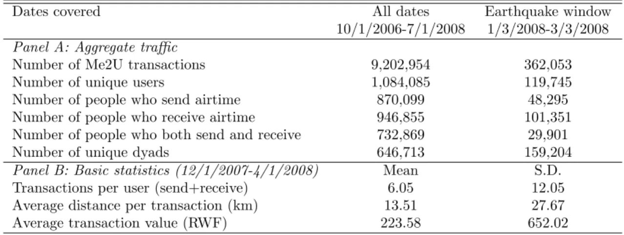
Table 2: Summary statistics of mobile network data.

Dates covered All dates Earthquake window

10/1/2006-7/1/2008 1/3/2008-3/3/2008

Panel A: Aggregate traffic

Number of Me2U transactions 9,202,954 362,053

Number of unique users 1,084,085 119,745

Number of people who send airtime 870,099 48,295

Number of people who receive airtime 946,855 101,351

Number of people who both send and receive 732,869 29,901

Number of unique dyads 646,713 159,204

Panel B: Basic statistics (12/1/2007-4/1/2008) Mean S.D.

Transactions per user (send+receive) 6.05 12.05

Average distance per transaction (km) 13.51 27.67

Average transaction value (RWF) 223.58 652.02

Notes: The window 10/1/2006-7/1/2008 encompasses the entire dataset with valid data on interpersonal airtime transfers. The window 1/3/2008-3/3/2008 is the same window used in later regressions. US$1=550RWF.

The main dataset used in our analysis is a log of all mobile-based airtime transfers that occurred between October 2006 and December 2009. For each transaction, the data contain unique identifiers for sender and receiver, the monetary value of the airtime sent, and the time and date at which the transfer occurred.

We also rely on a related data set that contains information about phone call activity. Every time a user makes or receives a phone call, the cell tower nearest to the user is logged. Since we also have records of the geo-coordinates of each cell tower, we can infer the approximate location of each mobile subscriber over time. Figure 1 depicts the spatial distribution of cell phone towers in early 2008 – the median area covered by a single cell phone tower is 72km2_{. Thus, for each user on each day, we infer that his location is the same} as the cell tower through which the majority of his calls were routed.11

Figure 2 shows the distribution of distances over which transfers are sent in the month prior to the Lake Kivu earthquake, for transactions involving at least one user in the earthquake region. While the vast majority of transfers are sent over a short distance, there are a large number of transfers sent to and from the capital of Kigali, which is approximately 150km from the epicenter. Additional summary statistics of the dataset are presented in Table 2.

B

Social networks and wealth index

For confidentiality reasons, each user in our dataset is anonymous and we do not observe basic demographic information such as the age, gender, or education level. We are nevertheless able to construct variables of interest based on phone usage. For instance, it is possible to compute the number of unique contacts

11_{Note that cellular coverage is not affected by topology to the same extent as radio transmitters as in Yanagizawa-Drott}

(2010). Using more sophisticated locational inference, such as the individual’s center of mass, does not have a noticeable effect on our results.

Figure 1: Map of Rwanda showing the location of mobile phone towers (as of February 2008) and the location of the Lake Kivu earthquake of 2008. Each black dot represents a cell tower, with the approximate area covered by the tower demarcated by adjacent Voronoi cells. The epicenter of the earthquake is shown with red concentric circles.

with whom a user has communicated over a given interval of time, as well as the geographic distribution of these contacts. Appendix A presents summary statistics of a number of social network variables that can be computed from the data.

Wealth is believed to play an important role in the way people share risk. As we saw in Section B, differences in wealth or permanent income are predicted to generate different patterns of transfers in the immediate aftermath of an emergency, depending on whether these transfers follow motives of charity or reciprocity, broadly defined. To construct a proxy for wealth we proceed in three steps as follows. The complete details of the procedure are described in (Blumenstock et al. 2010).

Using a Demographic and Health Survey of 10,000 households with detailed consumption and expen-diture information (Government of Rwanda, 2008), we first estimate a predicting equation for the annual expendituresYidof householdiin districtd. This equation captures the relationship betweenYidand various

Distribution of distance between sender and recipient (km) Distance in kilometers Density 0 50 100 150 200 0.00 0.02 0.04 0.06 0.08 0.10

(a) Distribution of distances

Distribution of distance between sender and recipient (km)

Distance in kilometers Density 0 50 100 150 200 0.00 0.02 0.04 0.06 0.08

0.10 _{2 months prior to earthquake} 2 days after earthquake

(b) Kernel density before/after quake Figure 2: Distribution of distances over which transfers are sent to and from the earthquake region.

The predicting equation:

Yid=α+ h∑max j βjHid+ a∑max k δkAid+µd+ϵid (7)

is estimated with district fixed effects using µd. From equation (7) we can estimate the predicted annual

expenditures Ybid of a household from the assets and durables Hid and assets Aid that it owns. Predicted

expenditureYbid is taken as proxy for permanent income.

In a second step, we use data from a phone survey to relate Hid and Aid to phone usage. The survey,

conducted by the authors, covers the random sample of approximately 900 mobile phone users used to generate Table 12. Basic demographic information was collected, together with data onHidandAid. Armed

withHidandAid it is possible to compute predicted annual expendituresYbid using coefficient estimates from

equation (7).

In the third step we compute, for each phone user, a vector of phone usage variables Xir thought to be

correlated with income, such as the total number of calls made and the average amount of airtime purchased over a given time interval: presumably richer individuals make more calls, and purchase airtime using larger denomination top-up vouchers. The variables are summarized in Table (12). Data on interpersonal transfers is excluded fromXir. We then fit a flexible model of the form:

b

and estimatef(.) using data from the phone user survey.12 Our wealth index is the predictedYbbid obtained

by applying the estimated flexible functionfb(.) to the full sample of 1.5 million phone users. This variable is used as proxy for wealth or permanent income when estimating heterogeneous effect equations (4) to (6).

4

Results

We now estimate regression models (1)-(3). The outcome of interest τijrt is the gross value of airtime

transferred from userj to useriin location ron dayt. To implement our testing strategy, we need a shock

Srtthat is exogenous to transfers on the mobile phone network. The primary shock that we exploit is a large

earthquake that occurred in the Western Rusizi and Nyamasheke districts of Rwanda on February 3, 2008. The magnitude 6 earthquake left 43 dead and 1,090 injured. It destroyed 2,288 houses and caused regional school closures and electrical outages. The effects of the earthquake, though large, were geographically circumscribed. The United States Geographical Survey estimates an impacted radius of approximately 20 kilometers from the epicenter – see Figure (1). This event is ideal for our estimation strategy since the shock is unequivocally exogenous and precisely located in time and space. We later demonstrate that our results are robust to using alternative shock measures including a severe flood that occurred in late 2007.

We begin by estimating equation models (1)-(3) to measure the causal impact of the earthquake on interpersonal transfers. We then turn to equation models (4) to (6) and test whether airtime transfers after the earthquake vary systematically across users.

A

Average effect of the earthquake

We first estimate equation (1) at the district level. The dependent variableτrtis the aggregated gross value

of transfers received on dayt in districtr. This value is obtained from the operator’s transaction logs by aggregating interpersonal transfers received by the cell tower of the receiver, and linking these towers to specific districts. We use data from 30 days before to 30 days after the earthquake, though as demonstrated in section 5 results our results change little if we use a different time window. District and day fixed effects are included as additional regressors to control for systematic differences across districts and over time. Results are presented in column (1) of Table 3. The earthquake shock variableSrt equals one on February

3rd 2008, the day of the earthquake, in the districts of Rusizi and Nyamasheke; it is zero otherwise. Robust standard errors are reported, clustered at the district level. The number of observations corresponds to a 60 day window over 30 districts.

12_{We experimented estimating functionf() in a number of ways. The results presented here rely on a simple linear regression}

Table 3: Average Effect of the Earthquake on Mobile Transfers Received (Gross)

(1) (2) (3) (4)

District Cell Tower User Dyad

Earthquake shock 14169*** 2832*** 9.48*** 11.92*** (1,951.30) (177.02) (0.74) (0.59)

Day dummies yes yes yes yes

Fixed effects district tower user directed dyad

Number of observations 1800 16020 6619440 10566000

Notes: *** p<0.01, ** p<0.05, * p<0.1. Standard errors, clustered by district, reported in parentheses.

We observe a strongly significant positive coefficient on the shock variable. The earthquake caused an additional influx of 14,169 Rwanda Francs (RWF), or approximately $28 USD. Though modest in absolute terms, this represents a large increase compared to an unconditional mean of 8,480 RWF in the two affected districts. It is also large relative to the average annual income of roughly $1,000 USD in Rwanda.

In the second column of Table 3, we repeat the analysis at the more disaggregated level of the cell tower. The number of cell towers (267) is larger than the number of districts (30), and this explains the larger number of observations. The advantage of estimating model (1) at the tower level is that each observation corresponds to a smaller geographical unit and thereby allows us to more precisely identify the regions affected by the quake. Tower fixed effects are included in the regression together with day-specific dummies. Again we find a statistically significant coefficient on the earthquake shock. Similar point estimates are produced if we redefine affected areas as those lying anywhere between 10 to 50 miles of the epicenter.

The earthquake produced an additional influx of approximately $84 USD to the 15 towers within 20km of the epicenter. This amount is small in absolute terms, but at the time of the earthquake, the mobile airtime transfer service had only recently been launched in Rwanda, and only 1,400 individuals living in the earthquake region had used the service prior to the earthquake. Since the earthquake, service utilization has increased over 400-fold. According to available information, there are currently 750,000 to 1,000,000 active users in Rwanda each day. This compares to 2,500 at the time of the earthquake. If we are willing to assume that airtime transfers following an earthquake increase proportionally to the number of active users, a similar earthquake today would cause an additional influx of US$22,000 to $30,000 to affected areas.13

The absolute value of transfers observed in February 2008 is also small because Rwanda is a small country with a population of ten million, less than one million of whom owned a telephone at the time of the earthquake. In Kenya the daily volume of money transferred over the mobile phone network is in excess of US$200 million, compared to US$1,500 in Rwanda at the time of the quake. Again, if we are willing to

13_{If emergency transfers are proportional to traffic and traffic increases non-linearly in the number of subscribers, as much}

of the network literature suggests, the projected amount may even be much larger. It is also conceivable, however, that early adopters are not representative of late adopters and respond more strongly to an earthquake; in this case, transfers need not increase proportionally with traffic or the number of users.

Table 4: Average Effect of the Earthquake on Mobile Transfers Received (Net)

(1) (2) (3)

District Cell Tower User

Earthquake shock 12823*** 3053*** 10.01***

(1600) (116) (1.082)

Day dummies yes yes yes

Fixed effects district tower user

Number of observations 1800 16020 6619440

Notes: *** p<0.01, ** p<0.05, * p<0.1. Standard errors, clustered by district, reported in parentheses.

assume that emergency transfers would increase proportionally to the total volume of airtime transfers, we would expect an influx of approximately US$11.2 million ($84×200M/1500) to affected districts.

Columns (3) and (4) repeat the estimation at the level of the individual user and of the dyadic pair of individuals. In the individual user regression (2), the dependent variable τirt is the amount of airtime

transfered to individual i in locationr at timet. Users who never receive airtime transfers are excluded since they do not help identify the effect of the shock, leaving roughly 110,000 unique individuals. The estimated coefficient is again positive and statistically significant. Results from the dyad-level regression (3) are presented in column (4) of Table 3. In this regression, pairs in which i never receives airtime from j

are ignored from the estimation, leaving roughly 180,000 valid dyads.14 Here too the shock coefficient is positive and statistically significant. The evidence is thus consistent: at all levels of aggregation we observe an increase in gross transfers.

As a robustness check, we redo the same analysis using net instead of gross transfers. The concern is that gross transfers may misrepresent the aggregate magnitude of the transfers if individuals who receive airtime pass it on to others in the same region. This could result in double-counting at the district or cell tower level. For the individual user regression (2) we redefine the dependent variable asτ_irt′ =∑_jτijrt−

∑

jτjirt,

that is, the transfers received byi from others minus the transfers given byito others. At the district and cell tower levels, we proceed as follows. Let τr1r2t =

∑

i_∈r1

∑

j_∈r2τijrt where r1 and r2 are two different

locations (e.g., districts or cell tower area); τr1r2t represents the total transfers received by individuals in

locationr1from individuals in locationr2. Summing over all other locations yields the gross transfers from other locations to locationr1. Net inflows to region r1 are thusτr′1t =

∑

r2τr1r2t−

∑

r2τr2r1t. We do not

replicate the dyadic regression since, in this case, net and gross transfers are indistinguishable.

Results, shown in Table 4, are not very different, both in terms of significance and in terms of magnitude, from those reported in Table 3. In the district level regression (column 1), the coefficient of the shock variable is slightly smaller than in Table 3. But in the regressions at the cell tower (column 2) and individual user

(column 3) levels, the coefficient is slightly larger. This implies that the magnitude of our findings is not driven by double counting.

B

Heterogeneous effects

We now introduce heterogeneous effects into the analysis. As outlined in Section B, we are looking for evi-dence of whether airtime transfers after the earthquake are best understood as a manifestation of reciprocity or charity. We have proposed three indirect tests: (1) if transfers are manifestation of charity, they are unlikely to flow from the poor to the rich; not necessarily so if they follow a reciprocal motive; (2) if transfers are embedded in reciprocal relationships, users with more such relationships should receive more after the shock; (3) if transfers are based on a reciprocal arrangement, they are expected to fall with the distance between giver and recipient because distance impinges observability and makes self-enforcing reciprocity arrangements harder to sustain.

The purpose of this section is to investigate these three predictions in our data by estimating the regression models (4) to (6). If people give primarily due to charitable motives, we expect transfers to flow primarily from rich to poor, from urban to rural, and to increase the further away the sending is from the shock. If people instead give primarily out of expectation of future reciprocity, we expect rich victims to receive more than poor, more transfers to take place between users already in a relationship, and transfers to decrease with the distance between sender and recipient.

Results for wealth are reported in Table 5. We worry that some users, especially richer users, may receive more airtime but also transfer more to others. We therefore use net transfers as the dependent variable. At the individual level we are using as wealth proxy the predicted expenditure variableYbbiddescribed in Section

3. At the district and cell tower levels, the wealth proxy is the sum of Ybbid over all users in that location.

To avoid spurious results, we also include interaction terms between the wealth proxy with the day of the earthquake and with a dummy for presence in the earthquake affected region.

The coefficient of interest is the coefficient of the interaction term between wealth and shock in the second row of Table 6. Results clearly show that richer users receive more airtime transfers in the immediate aftermath of the earthquake. The estimated coefficient is largest in the user and dyad regressions, which is what we would expect. In the dyad regression we are also able to include an interaction term with the wealth of the sender. This term is not significant.

These findings are difficult to reconcile with a pure charity/altruistic motive. However, they are consistent with transfers being embedded in reciprocal relationships in which people receive in-kind gifts they value – in this case, airtime at a moment when better-off users wish to call relatives or emergency services. This

Table 5: Net transfers and wealth

(1) (2) (3) (4)

District Cell Tower User Dyad

Earthquake shock 24,121*** 4,906*** 12.53*** 14.25***

(1,531.00) (978.52) (3.40) (3.28) Wealth proxy of recipient * Shock 1.936*** 2.041** 17.57*** 13.69***

(0.15) (0.96) (5.14) (2.13)

Wealth proxy of recipient * Day of quake -0.315** -0.079 -1.32*** -0.54

(0.15) (0.18) (0.20) (0.40)

Wealth proxy of recipient * In quake region 1.38* 0.17

(0.73) (0.38)

Wealth proxy of sender * Shock 6.00

(6.00)

Wealth proxy of sender * Day of quake 0.63*

(0.37)

Wealth proxy of sender * In quake region 0.03

(0.42)

Day dummies yes yes yes yes

Fixed effects district tower user directed dyad

Number of observations 1800 16020 6619440 10566000

Notes: *** p<0.01, ** p<0.05, * p<0.1. Standard errors, clustered by district, reported in parentheses.

interpretation finds additional support from observing that individuals with a higher value ofYbbidalso receive

more airtime transfers on days other than the earthquake day.15

To further investigate the importance of relationships, we interact the earthquake shock with a proxy for the social network of the recipient, namely the number of unique individuals with whom the person communicated over the phone in the year prior to the earthquake. The number of contacts an individual has does not necessarily imply that the person is in more reciprocal favor-exchange relationships, but the two may be correlated.

Results are shown in Table 6. As before, district and cell tower values are the sum of the degree of recipients in that location. The coefficient of interest, that for the interaction term between the shock and the degree of the recipient, is positive throughout but only significant in the district and cell tower regressions. In the dyadic regression we also include interaction terms for the degree of the sender. The coefficient of the interaction term with the shock has the expected sign but is not statistically significant. Similar findings obtain with different measures of the recipient’s social network, e.g., the number of unique individuals the user has called, the number of unique individuals who called the user, the number of international contacts, and the number of contacts with whom the user sent or received airtime. From this we conclude that there is only mild evidence that the size of users’ social network matters at the time of the earthquake.

Next we investigate whether individuals receive more in the aftermath of the earthquake if they are in

15_{These results, not shown, are obtained by regressing individual fixed effects on the uninteracted covariates (in this case,}

Table 6: Net transfers and number of contacts

(1) (2) (3) (4)

District Cell Tower User Dyad

Earthquake shock 24,381*** 4,631*** 12.24*** 13.36***

(721.13) (415.26) (3.56) (2.58)

Degree of recipient * Shock 0.004*** 0.004** 0.05 0.03

(0.00) (0.00) (0.03) (0.03)

Degree of recipient * Day of quake 0.000 -0.000 -0.00*** -0.00

(0.00) (0.00) (0.00) (0.00)

Degree of recipient * In quake region 0.01* 0.00

(0.01) (0.00)

Degree of sender * Shock 0.01

(0.01)

Degree of sender * Day of quake 0.00

(0.00)

Degree of sender * In quake region -0.00*

(0.00)

Day dummies yes yes yes yes

Fixed effects district tower user directed dyad

Number of observations 1800 16020 6619440 10566000

Notes: *** p<0.01, ** p<0.05, * p<0.1. Standard errors, clustered by district, reported in parentheses.

relationships with a strong favor-exchange component. To this effect, we reestimate the dyad-level regression presented in column (4) of Table 6, replacing the degree of the recipient with the accumulated amount of transfers the recipients has received and given in the past. Reciprocal relationships are those in which we observe a history of transfers, and the stronger this history of transfers, the stronger we expect the favor-exchange relationship to be. Because we wish to focus on the nature of the relationship, we focus on dyadic-level regressions.

Results are presented in Table 7. We see that individual i who has sent more airtime to individual j

in the past receives more help fromj on the day of the earthquake. Having received airtime fromj in the past is not significant. This is consistent with a reciprocal relationship: ihas transferred airtime toj andj

reciprocates at the time of the earthquake wheni is most likely to need help.

Finally, as discussed in Section 2, we also investigate whether transfers come uniformly from other unaffected regions of Rwanda, or whether transfers come primarily from unaffected areas in the vicinity of the earthquake. If transfers follow primarily a charitable motive, we expect all unaffected areas to contribute; not so if transfers are motivated by reciprocity, and relationships are strongest with people nearby. To examine this possibility, we disaggregate each individual’s social network by distance. We first divide the number of contacts of each useriinto different groups, each corresponding to a distance range fromi’s location, with distance ranging from 0 Km to 250 Km. We then interact each of these variables with the earthquake shock and examine the transfers received by individual iin regression (5). Results are shown in Appendix Table

Table 7: Net transfers and past reciprocity

Dyad Dyad (with FE)

Earthquake shock 12.095*** 11.898***

(0.948) (0.702) Airtime sent in the past (fromitoj) * Shock 0.462*** 0.476***

(0.124) (0.119) Airtime sent in the past (fromitoj) -0.172***

(0.009)

Airtime sent in the past * Day of quake 0.056 0.057 (0.041) (0.042) Airtime sent in the past * In quake region 0.139*** 0.129* (0.050) (0.073) Airtime received in past (byifromj) * Shock 0.138 -0.167

(0.251) (0.278) Airtime received in past (byifromj) 1.034***

(0.038)

Airtime received in the past * Day of quake -0.212*** -0.215*** (0.037) (0.054) Airtime received in the past * In quake region -0.328*** -0.277

(0.121) (0.195)

Day dummies yes yes

Fixed effects no directed dyad

Number of observations 10566000 10566000

Notes: Outcome isτijrt, i.e. the airtime received byifromjon dayt. *** p<0.01, ** p<0.05, * p<0.1. Standard errors, clustered by district, reported in parentheses.

13.

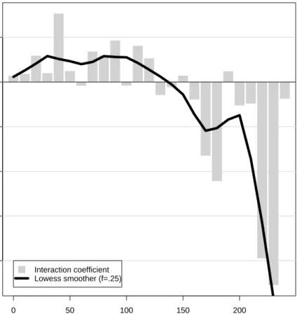
We first note that, if we omit individual fixed effects, we find that the number of contacts at any distance is correlated with the amount of money received in the absence of earthquake. This indicates that individuals with more contacts are more likely to receive transfers in general. When we interact distance-specific degree with the shock, however, results are different. We plot in Figure 3 the interaction coefficients by distance, together with a locally-weighted polynomial smoother to more clearly show the non-parametric relationship between earthquake-induced transfers and distance. We observe that after the quake, people with many contacts near the epicenter do not receive more transfers, presumably because nearby friends are also affected by the earthquake. People with contacts more than 30 Km away from the epicenter are more likely to receive transfers in the aftermath of the earthquake, but the effect dies down for contacts located more than 100 Km from the epicenter. This pattern is consistent with the predictions of a model of reciprocation in which information and monitoring costs increase with distance and close range relationships therefore include a stronger mutual insurance element.

0 50 100 150 200 −2.0 −1.5 −1.0 −0.5 0.0 0.5

Distance from recipient

Shock X Distance coefficient

Interaction coefficient Lowess smoother (f=.25)

Figure 3: Relationship between the geographic structure of an individual’s network and her propensity to receive a transfer after the earthquake.

5

Robustness and Limitations

A

Functional form assumptions

We briefly show that our central results are not sensitive to the precise econometric specifications, or to the choice of time window (which in most regressions is restricted to the period starting one month before the earthquake and ending one month after the earthquake). Table 8 presents estimates of the average treatment effect of model (1) using the full dataset from October 2006 until July 2009 under a variety of econometric specifications. Column (1) gives the standard OLS results with no control variablesXrt, time fixed effects

θt, or tower fixed effects πr. Column (2) includes time-varying controls to account for regional variation

in mobile phone use, column (3) adds regional fixed effects, and column (4) adds daily dummy variables. Across all specifications, the estimated effect of the shock remains strong and significant, and of a magnitude similar to that presented in Table 3.

Table 8: Sensitivity of estimation to function form assumptions

(1) (2) (3) (4)

Pooled OLS OLS w/Controls Region FE Region & Day FE

Shock 1793.639*** 2819.503*** 2787.305*** 2710.861*** (313.08) (121.33) (136.18) (183.53) Day of quake -748.548** -1375.294*** -1287.145*** (212.87) (111.76) (119.77) In quake region -2262.728*** -510.751*** (577.57) (73.57)

Total call volume 0.074*** 0.064*** 0.103***

(0.00) (0.01) (0.01)

Outgoing transfers 0.677*** 0.637*** 0.527***

(0.03) (0.03) (0.04)

Tower Fixed Effects No No Yes Yes

Date Fixed Effects No No No Yes

R2 _{0.008 0.702 0.729 0.753}

N 171414 74895 74895 74895

Notes: Outcome is the total amount transferred into a tower on a single day. “In quake region” defined as those towers within 20 miles of the earthquake epicenter. Columns 2-4 include controls for overall network activity. Column 3 includes tower-level fixed effects. Column 4 includes daily fixed effects. Estimates made using data from October 1, 2006 through July 1, 2008. Heteroskedasticity-robust SE’s in parentheses (clustered at district level). * p<0.05, ** p<0.01, *** p<0.001.

B

Standard errors

As discussed in Section 2, for standard error estimates to be consistent in the dyadic regressions, they should ideally be cross-clustered by senderiand recipientj. This is because transfers involving the same individual are likely to be correlated with each other – e.g., ifj transfer airtime toi, he is ceteris paribus less able to transfer airtime to others. In the results presented so far we have clustered standard errors by the district in which the recipient resides.

As a robustness check, Table (9) compares alternative methods of obtaining standard errors using different levels of clustering: no clustering (column 1), by recipient (column 2), by sender (column 3), and by date (column 4). Standard errors are largest when we cluster by recipient, but in all specifications the coefficients of interest are highly significant. In the last column of Table (9), we drop observations in such a way that each senderj appears only once. More precisely, whenever a senderj appears multiple times, only one dyad involving j is selected at random and kept for estimation purposes. This results in a smaller number of observations but it eliminates the problem of correlation of errors at the source. The standard error is larger – if only because we dropped observations – but the coefficient of interest remains significant.

Table 9: Robustness of dyadic results

(1) (2) (3) (4) (5)

Clustering None Recipientj Senderi Dayt Unique senders

Shock (recipient) 7.395* 7.395† 7.395* 7.395*** 6.923*

(3.70) (3.77) (3.77) (0.19) (2.67)

Priorτji (last month) -2.541*** -2.541*** -2.541*** -2.541*** -2.621***

(0.19) (0.20) (0.22) (0.64) (0.33)

Priorτji * Shock 20.560 20.560 20.560 20.560*** 50.361

(16.80) (17.00) (17.07) (0.86) (38.91)

Day fixed effects Yes Yes Yes Yes Yes

Dyad fixed effects Yes Yes Yes Yes Yes

R2 0.055 0.055 0.055 0.055 0.053

N 4868562 4868562 4868562 4868562 2720077

Notes: Specification is identical to that used to produce Table??, but standard errors are clustered according to column labels. Column (5) clusters by recipient, but restricts sample to allow only one recipient per sender. In cases were a single sender sends to multiple recipients, one recipient is chosen at random and the others are dropped from the analysis. † p<0.10, * p<0.05, ** p<0.01, *** p<0.001.

C

Placebo tests

As a robustness check of the average treatment effect, we verify that the effects of the earthquake on transfers are unique to the day of the earthquake, and do not generally occur on days without significant economic shocks. We do this first at the district level, following the methodology used to produce Table 3. In Appendix Table 14, we include lag and lead terms to test whether there was a significant effect of the earthquake on transfer patterns in the days immediately before and after the earthquake. To identify these ten additional terms, we include district-level data from the full dataset as in Table 8. In column 1, we observe that this effect does not exist, and before the earthquake (lead1-lead3) and after the earthquake (lag1-lag7), there was no significant change in transfers to the affected regions. These results hold for lags and leads of up to 10 days. In columns (2) and (3), we see in contrast that national calls to the affected region increase in the days following the earthquake. International calls do not. Critically, there was no anomalous increase in any sort of mobile network traffic in the days prior to the earthquake.

Appendix Table 15 presents results from testing the same specification as in column 4 of Table 3 but with a “placebo” shock at the same location on different dates. Thus, we test for a spurious effect 1 and 2 months before, as well as 1 month after, the actual earthquake. In contrast to the results obtained for the date of the actual earthquake, we observe no significant change in transfers on the day of the placebo earthquakes.

D

Other large covariate shocks

The results presented so far provide strong evidence that Rwandans used the mobile phone network to send airtime to friends and families affected by a major earthquake, and that these results are robust to different empirical specifications. We now show that similar transfers are observed following other natural disasters.

During the period for which we have mobile phone data, there were no massive natural disasters on the scale of the Lake Kivu earthquake. However, there were two major floods that severely disrupted the lives of many Rwandans. These floods are not as well suited to our estimation strategy as the earthquake, since floods are less precisely located in space (there is no single epicenter), and the timing is only partially exogenous (prior weather patterns anticipate floods). Therefore, there are a priori reasons to expect that the effect of a flood on transfers would be less pronounced than the effect of an earthquake.

Nonetheless, we do observe a significant increase in transfers on the days following a severe flood. In Table 10, we estimate equation (1) for the towers in the region of a flood that killed 17 during September 2007. We find a modest but strongly significant increase in airtime sent to regions affected by the flood. In column (4) of Table 10, the point estimate is roughly half that of the corresponding point estimate of the effect of the earthquake (column 4 of Table 8).

Table 10: Effect of flood on transfers

(1) (2) (3) (4)

Pooled OLS OLS controls tower FE tower/Time FE

shock 1456.901 933.040∗∗ 1029.241∗∗ 1068.659∗∗ (770.84) (316.98) (329.36) (375.45) Days of flooding 774.798∗∗∗ 952.838∗∗∗ 981.247∗∗∗ (166.92) (230.79) (206.75) In flooded region 263.474 237.740∗ (919.80) (88.55) Total calls 0.075∗∗∗ 0.065∗∗∗ 0.103∗∗∗ (0.00) (0.01) (0.01) Outgoing transfers 0.678∗∗∗ 0.637∗∗∗ 0.527∗∗∗ (0.03) (0.03) (0.04) R2 _{0.000 0.702 0.729 0.753} N 171414 74895 74895 74895

“In flood region” defined as towers in the two districts affected by the flood. “Days of flood” are 9/12/07 - 9/18/07.

E

Limitations

One limitation of our empirical strategy is the fact that we are not able to observe transfers that occur outside of the mobile phone network. Thus, it is possible that the effect we observe is merely one of substitution, and that individuals who send money over the network would have sent it using another mechanism. While

Table 11: Alternative services for transferring money Alternative Service Estimated Fees

(small transfers)

Availability Source

MoneyGram 7% - 100%

($15 minimum)

5 locations MoneyGram Website, 2010;

Orozco, 2009

Western Union 10%-100%

($10 minimum)

50 locations Western Union Website, 2010;

Orozco, 2009

Post Office 8%-1% 19 branches World Bank Group, 2009;

Remit-tance Tanzania to Rwanda; Mu-goya, 2009

Commercial Bank 6%-40% Urban and semi-urban areas World Bank Group, 2009; Remit-tance Tanzania to Rwanda

Bus 6% - 20% Populous areas Kbbucho, et al. 2003; Kenya

Money Transfer Rates; Averaged over Bus-Star/Scandinavian Friends/Relative No fee, no

stan-dard system

Depends on social network Kbbucho, et al. 2003 Mobile-based transfers Free 3 million phones

we cannot reject this interpretation empirically, we note that at the time of the earthquake, there were very few alternative methods for transferring money over distance. These alternatives are summarized in Table 11. MoneyGram, Western Union, and the Post Office are the other official methods for transferring money, but transaction costs across these services range from 10 - 100% of the value of the money sent. For each of these services, it is impossible to transfer amounts under US$10. In the informal sector, the most common method for transferring money is by bus/taxi, but for that service the driver typically charges 10-20% of the amount transferred, and the availability of the service is contingent on the schedule of busses and the condition of the roads. With the mobile transfer service, by contrast, the transfer of money is instantaneous and has no associated fees or commissions.

An additional caveat of our analysis regards the utility of a mobile phone-based transfer in comparison to a transfer of hard cash. During the time period we analyze, the mobile-based transfer system only allowed for the transfer of airtime from one individual to another. Though the current system allows for the transfer of money, which can be converted to cash or spent directly at many small stores, this was not the case in early 2008. Thus, the transfers received by the victims of the earthquake were less liquid than a transfer of money handed from one person to another.16 However, as mobile banking services are more fully developed, these transaction costs are expected to be greatly reduced.17 _{It therefore seems plausible that our estimates} represent a lower bound on the amount of money that would be sent over the mobile network in response

16_{Whether the transfer is more or less liquid than a formal transfer over a service such as Western Union is ambiguous. Even}

in 2008, airtime could easily be converted to cash through local resellers. Moreover, given the aforementioned evidence that as much as 20% of household expenditures were on mobile phone-related expenses, it is likely that a transfer of airtime would lead to inframarginal savings on the part of the recipient.