Robust Value at Risk Prediction
∗Loriano Mancini Swiss Finance Institute
and EPFL
Fabio Trojani Swiss Finance Institute and University of Lugano
This version: 10th September 2010
∗Correspondence Information: Loriano Mancini, Swiss Finance Institute at EPFL, Quartier UNIL-Dorigny,
CH-1015 Lausanne, Switzerland, phone: +41 (0)21 693 0107, fax: +41 (0)21 692 3435, E-mail: [email protected]. E-mail address for Fabio Trojani: [email protected]. For helpful comments we thank Eric Renault (the editor), the associate editor, two anonymous referees, Claudio Ortelli, Franco Peracchi, and Claudia Ravanelli.
Robust Value at Risk Prediction
Abstract
This paper proposes a robust semiparametric bootstrap method to estimate predictive distribu-tions of GARCH-type models. The method is based on a robust estimation of parametric GARCH models and a robustified resampling scheme for GARCH residuals that controls bootstrap instability due to outlying observations. A Monte Carlo simulation shows that our robust method provides more accurate VaR forecasts than classical methods, often by a large extent, especially for several days ahead horizons and/or in presence of outlying observations. An empirical application confirms the simulation results. The robust procedure outperforms in backtesting several other VaR prediction methods, such as RiskMetrics, CAViaR, Historical Simulation, and classical Filtered Historical Sim-ulation methods. We show empirically that robust estimation reduces tail estimation risk, providing more accurate and more stable VaR prediction intervals over time.
Keywords: M-estimator, Extreme Value Theory, Breakdown Point, Backtesting.
Introduction
Large portfolios of traded assets held by many financial firms have made the measurement of market risk, i.e. the risk of losses on the trading book due to adverse market movements, a primary concern for regulators and risk managers. The Basel Committee (1996) requires that financial firms hold a certain amount of capital against market risk. This capital is called Value at Risk (VaR) and must be sufficient to cover losses on the trading book over a ten days holding period 99% of the times. In practice, VaR is computed for several holding periods and confidence levels, such as 95% confidence level and horizon of one day. From a statistical viewpoint, VaR is the quantile of the profit and loss (P&L) distribution of a portfolio over a certain holding period. Hence, a key issue in implementing VaR and related risk measures is to obtain accurate estimates for the tails of conditional P&L distributions. Semiparametric methods, commonly called Filtered Historical Simulation (FHS) methods, have been found to provide rather accurate estimates of P&L distributions; see for e.g. Pritsker (1997), Hull and White (1998), Diebold, Schuermann, and Stroughair (1998), Barone-Adesi, Giannopoulos, and Vosper (1999), McNeil and Frey (2000), Pritsker (2001), and Kuester, Mittnik, and Paolella (2006). In FHS methods, parametric GARCH-type models are typically fitted to historical returns using pseudo maximum likelihood (PML). Then GARCH residuals are resampled using bootstrap methods. The FHS methods allow for time varying conditional moments of returns (via GARCH-type models) and nonparametric structures in conditional distribution of returns (because innovation distributions are estimated nonparametrically). The last feature is crucial in applications and avoids too simplistic assumptions on return conditional distributions, such as normality; see e.g. JP Morgan’s RiskMetrics (1995).
In this paper we propose a general robust semiparametric bootstrap method to estimate predictive distributions of asset returns in GARCH-type volatility models. The method allows for general para-metric specifications of time varying conditional mean and volatility of asset returns. As an application, we use the proposed robust method to predict Value at Risk over different forecasting horizons. Our
approach achieves robustness in two steps. In the first step, we estimate a parametric GARCH-type model using the optimal bounded influence estimator in Mancini, Ronchetti, and Trojani (2005). In the second step, we fit generalized Pareto distribution using the robust estimator in Dupuis (1999) and Ju´arez and Schucany (2004) to the tails of GARCH residuals distribution and we resample from this distribution. In order to ensure robustness of the whole procedure, both robustification steps are necessary.
PML estimators with Gaussian pseudo densities are often used to fit GARCH-type models and they feature a number of convenient theoretical properties. For instance, they achieve maximal efficiency (be-ing ML) when returns are indeed conditionally Gaussian. Moreover, even under non Gaussian returns, they imply consistent estimation of the parameters in the conditional mean and variance functions, provided the latter are correctly specified. Finally, in some cases Gaussian PML estimators coincide with weighted nonlinear least squares estimators and can achieve the semiparametric efficiency bound for estimating a correctly specified conditional moment function.
In the more general situation of (i) potentially misspecified conditional mean and variance functions and (ii) non Gaussian returns, these convenient properties of PML can break down. In this case, PML implicitly estimates a pseudo true value for the conditional GARCH-dynamics, which minimizes the Kullback–Leibler discrepancy between the unknown conditional density of returns and a parametric family of Gaussian pseudo likelihoods. A major issue is that even if the relevant degree of misspecification might be small, in the sense that the true conditional moments of the data generating process might be only slightly different from those specified under the parametric GARCH assumption, there is no guarantee that the conditional moment function implied by the theoretical pseudo true value will again be only slightly different from the true one; see, e.g., Sakata and White (1998) and Mancini, Ronchetti, and Trojani (2005) for some concrete evidence on this point. Similarly, under such circumstances there is no guarantee that PML can produce estimates of the pseudo true conditional mean and variance functions that are comparably efficient as in the case of a correct specification of the latter. These
features of Gaussian PML are strongly related to the functional structure of these estimators, which implies excess sensitivity of pseudo true values and PML asymptotic covariance matrices with respect to the underlying data distribution. Such a sensitivity or non-robustness of these estimators can be problematic because even a moderate misspecification of the assumed parametric model can lead to either strongly biased or inefficient results, e.g., in terms of the implied mean square error for the estimated conditional moments.
In this paper, we apply a class of robustM-estimators for GARCH-type models proposed in Mancini, Ronchetti, and Trojani (2005). These estimators ensure smoothness of the implied pseudo-true value with respect to the underlying data distribution using a set of robustified moment conditions defined by a bounded estimating function. The robust estimating function is obtained from the Gaussian PML score function by a down-weighting procedure. This procedure bounds the potential damaging effects of data points generating a large sensitivity of theoretical PML pseudo true values with respect to the underlying data distribution. Our estimators provide robust, i.e., smooth, estimation results in an abstract nonparametric neighborhood of a fixed reference model, which we take to be a GARCH-type model with Gaussian errors. In general, a trade-off between robustness (with respect to model misspecification) and efficiency (under a correct model specification) emerges when choosing between robust and PML estimators, and the researcher has to decide on this trade-off. It is an empirical question whether the quantitative effects of a small misspecification of GARCH-type models, e.g., in the form of an incorrect variance dynamics, can lean the trade-off in favor of using robust methods in the estimation of GARCH-models for predicting VaR. Sakata and White (1998) and Mancini, Ronchetti, and Trojani (2005), among others, show that such a favorable trade-off exists when estimating conditional variance dynamics already under a moderate model misspecification. In our Monte Carlo simulations, we find that robust GARCH estimators combined with a robust extreme value estimator for the conditional tails of returns produce lower mean square errors in forecasting the true VaR already under very small misspecifications of the assumed parametric model.
The issue of the impact of a model misspecification on the statistical properties of an estimator is even more pronounced when fitting innovation tail distributions, as required for VaR predictions. For instance, Generalized Pareto distribution (GPD) is typically used in Extreme Value Theory to model tail distributions of returns above a given threshold. Theoretically, the GPD is an asymptotic approximation of the tail, which improves in the limit as the threshold goes to infinity (or to the endpoint of the distribution). In practice, however, the threshold is fixed and the error implied by the GPD approximation for the true tail distribution can have nontrivial consequences for the properties of PML estimators based on a GPD pseudo density. This is so because the GPD PML score leads to an unbounded estimating function that implies nonsmooth pseudo true values with respect to variations of the underlying data distribution. In this context, the robust GPD estimator in our approach is a natural estimator, because it is based on a bounded estimating function that explicitly downweights the damaging effects of a potential misspecification of the tail specified by the GPD, thus providing more accurate estimators when such deviations are indeed present in the data. We confirm this intuition in several Monte Carlo simulations, showing that robust GPD estimator provides more accurate quantile estimates (e.g., in terms of a lower mean square error) under a number of realistic specifications of the tail. These estimates are also much less sensitive to the choice of threshold levels than classical methods. The latter is a further desirable property of the robust estimator, because in applications the selection of the threshold level is a difficult task.
Another important issue is the nonrobustness of several resampling procedures used to compute VaR estimates at several days ahead horizons. It has been recognized that a few large observations are sufficient to cause the breakdown of quantile estimates based on nonparametric residual bootstrap; see, among others, Singh (1998), Gagliardini, Trojani, and Urga (2005), Davidson and Flachaire (2007), and Camponovo, Scaillet, and Trojani (2009, 2010). We find that standard nonparametric bootstrap procedures for VaR computation have a very low breakdown point, meaning that VaR forecasts can be heavily affected already by a few large observations, especially when longer forecast horizons of,
e.g., ten days are considered. Using, the robust GPD estimator in our approach, we are also able to develop a resampling procedure for VaR forecasting that controls for the instability generated by outlying observations in estimated GARCH residual distributions; see also Cowell and Victoria-Feser (1996).
We perform an extensive Monte Carlo simulation and show that our robust method provides more accurate VaR predictions than classical methods under conditionally non Gaussian data, in particular for several days ahead horizons. When the GARCH model used to predict VaR is not exactly the same as the true data generating process, robust VaR predictions have mean square prediction errors several times smaller than those of classical procedures. In nearly all Monte Carlo experiments, our robust procedure has the lowest mean square prediction errors, often by a large extent. In contrast to classical methods, our procedure never fails validation tests at 10% confidence level.
The simulation evidence is confirmed by the real data application. We backtest VaR prediction methods using about twenty years of S&P 500, Dollar-Yen, Microsoft and Boeing historical returns. We compare our method to several alternative VaR prediction procedures, such as (i) Historical Simulation, (ii) RiskMetrics, (iii) Engle and Gonzalez-Rivera (1991) semiparametric GARCH model, (iv) Engle and Manganelli (2004) CAViaR model, and for 10-day ahead VaR predictions, (v) GARCH model applied directly to 10-day asset returns. Only our robust method passes all validation tests at 10% confidence level. Moreover, we find that the reduction in tail estimation risk of our robust procedure provides more accurate and more stable VaR prediction intervals over time. For instance, in the case of S&P 500 and Boeing, robust VaR prediction intervals are nearly 20% narrower and 50% less volatile than classical ones. Given the higher accuracy of robust VaR predictions documented in violation tests, the stability over time of robust VaR profiles is a feature that allows financial firms to adapt properly risky positions to VaR limits more smoothly and thus more efficiently.
Section 1 introduces classical and robust semiparametric bootstrap methods for VaR predictions. Section 2 presents Monte Carlo evidence on VaR predictions, under different forms of conditional non
normal returns. Section 3 presents the real data application and backtesting for four financial time series. Section 4 concludes.
1
Setting
1.1 Return Dynamics and Measures of Market Risk
LetY:={Yt}t∈Zbe a strictly stationary time series process on probability space (R∞,F,P∗), modelling
the daily rate of return on a financial asset with price Pt at time t, i.e. Yt :=Pt/Pt−1−1. We assume that distribution P∗ can be “approximated” by a parametric reference model Pθ0 in the parametric
familyP :={Pθ, θ ∈Θ⊆Rp}. Even if P∗ might not be a member of P, so that the parametric family
is misspecified, we assume thatP∗ belongs to a nonparametric neighborhood ofPθ0, denoted byU(Pθ0).
The neighborhood is assumed to be small, in the sense that the distribution distance between P∗ and Pθ0 is assumed to be moderate.
Remark 1.1 Neighborhood U(Pθ0) can be defined using different metrics between distributions, and it
represents a proximity of similar models used to provide an approximate statistical description of P∗. Robust estimators are designed to provide a smooth statistical behavior over neighborhood U(Pθ0), in
order to make the estimator’s properties not excessively dependent on which specific direction of mis-specification of Pθ0 might indeed be present in the data. In applications, the specific size of neighborhood
U(Pθ0) is in most cases only implicitly fixed by the degree of robustness imposed on the estimator used.
Intuitively, the more robust an estimator the broader the implicit neighborhood of potential model mis-specifications that are considered as possible relevant data generating processes in the robust approach.
Under Pθ0, we assume that processY satisfies the dynamic model
Yt=µt(θ0) +σt(θ0)Zt, (1)
whereµt(θ0) andσ2t(θ0) parameterize the conditional mean and conditional variance of Yt, given
GivenY1m :={Y1, . . . , Ym}, denote byP∗m(Pmθ0) them-dimensional marginal distribution ofY1m underP∗ (Pθ0). Ft,t+h is the conditional distribution function of h days returns Yt,t+h :=Pt+h/Pt−1 under P∗,
given information Ft. For 0< α <1 and horizonh days, let yt,tα+h denote theα-quantile ofFt,t+h, i.e. yt,tα+h := inf{y ∈ R : Ft,t+h(y) ≥ α}. For an asset with market price Pt, the Value at Risk (VaR) at
time t, confidence level α, and horizonh days, VaRαt,t+h, is defined by1
α=P∗(Pt+h−Pt<−VaRαt,t+h|Ft). (2)
Hence, −VaRαt,t+h = Ptyt,tα+h is the α-quantile of the conditional profit and loss (P&L) distribution
under P∗ over the next h days, given Ft.2 Another measure of market risk is the Expected Shortfall
(ES, Artzner, Delbaen, Eber, and Heath (1999)), St,tα+h := E∗[Yt,t+h|Yt,t+h < yt,tα+h,Ft], where E∗[·]
denotes expectation with respect to P∗. For horizonh= 1 day,
yt,tα+1=µt+1(θ0) +σt+1(θ0)zα, St,tα+1 =µt+1(θ0) +σt+1(θ0)E∗[Z|Z < zα],
wherezαis theα-quantile of the distribution ofZ. Estimation of VaR or ES can be obtained by
estimat-ing model (1) and tail distribution of residualsZ. For longer horizonsh≥2, estimating model (1) is only the starting point to compute market risk measures. Joint conditional distributions of{Zt+1, . . . , Zt+h},
{µt+1, . . . , µt+h}and{σt+1, . . . , σt+h}have to be estimated, a task which is considerably more difficult.
Filtering Historical Simulation (FHS) methods estimateFt,t+h using semiparametric bootstrap of model
(1) over horizon [t, t+h]. Our goal is to develop robust semiparametric bootstrap methods for estimating
Ft,t+h.
1.2 Estimation of GARCH-type Models
The parameters of model (1) are usually estimated by pseudo maximum likelihood (PML); see White (1982), Gouri´eroux, Monfort, and Trognon (1984), and Bollerslev and Wooldridge (1992). The func-tional PML estimator (PMLE) a(·) is defined by
where the Gaussian score function s(Y1m;θ) := 1 σ2 m(θ) ∂µm(θ) ∂θ εm(θ) + 1 2σ2 m(θ) ∂σ2m(θ) ∂θ ( ε2m(θ) σ2 m(θ) −1 ) (3)
and εm(θ) := σm(θ)Zm. PMLE has a number of convenient and useful properties. First, when true
distribution,P∗, coincides withPθ0, PMLE is indeed MLE. Second, if the conditional mean and variance
functions µm(θ0) and σm2(θ0) are correctly specified, they are consistently estimated even under non
Gaussianity of the errors distribution. However, an important issue is that even when the degree of misspecification might be small, e.g., with true conditional moments that might be only slightly different from those under the parametric model, there is no guarantee that the pseudo true conditional moments will remain only slightly different from the true ones. This feature of Gaussian PML is determined by the functional structure of these estimators, which implies excess sensitivity of pseudo true values and PML asymptotic covariance matrices with respect to the underlying data distribution. Such a sensitivity or non-robustness of these estimators is due to the fact that the estimating function of Gaussian PMLE is unbounded.
In this paper, we apply a class of robustM-estimators for GARCH-type models proposed in Mancini et al. (2005). These estimators ensure smoothness of the implied pseudo true value with respect to the underlying data distribution using a set of robustified moment conditions implied by a bounded estimating function. The robust estimating function is obtained from the Gaussian PML score function by a down-weighting procedure that bounds the potential damaging effects of data points generating a too large sensitivity of Gaussian PML pseudo true values.
Mancini, Ronchetti, and Trojani (2005) robust estimator is efficient and computationally feasible for highly nonlinear models, and compares favorably with other robust estimators, such as robust GMM estimators (Ronchetti and Trojani (2001)) or robust EMM estimators (Ortelli and Trojani (2005)) for time series. It is defined as follows. Let
ψc(s(Y1m;θ)) :=A(θ)
(
where s(Y1m;θ) is the PML score function defined in (3), and
w(Y1m;θ) := min(1, c∥A(θ)(s(Y1m;θ)−τ(Y1m−1;θ))∥−1).
The robust functional M-estimatora(·) ofθ is defined by
E∗[ψc(s(Y1m;a(Pm∗ )))] = 0, (5) where non singular matrix A(θ)∈ Rp×Rp and Fm−1-measurable random vectorτ(Y1m−1;θ) ∈Rp are determined by the implicit equations
Eθ0[ψc(s(Y m 1 ;θ0))ψc(s(Y1m;θ0))⊤] = I, (6) Eθ0[ψc(s(Y m 1 ;θ0))|Fm−1] = 0. (7) The estimating function ψc is a truncated version of PML score function (3) because by construction
∥ψc(s(Y1m;θ))∥ ≤ c. The constant c controls for the degree of robustness. When c = ∞, the robust estimator ain (5) is indeed the PMLE. Section 1.5 discusses how to select c.3
To obtain VaR predictions, conditional mean and conditional volatility in model (1) have to be specified; see e.g. Ghysels, Harvey, and Renault (1996). Several GARCH-type models have been pro-posed in the financial literature. Our robust method can accommodate general specifications forµt(θ0)
and σt(θ0) that imply different estimating functions but do not change the overall procedure. In our
simulations and empirical applications, we adopt a fairly flexible model, namely an AR(1) model for the conditional meanµt(θ0) and an asymmetric GARCH(1,1) model for the conditional varianceσ2t(θ0)
(Glosten, Jagannathan, and Runkle (1993)),
µt(θ0) = ρ0+ρ1Yt−1, (8)
σ2t(θ0) = α0+α1ε2t−1(θ0) +α2σt2−1(θ0) +α3ε2t−1(θ0)It−1(θ0), (9)
where α0, α1, α2 > 0, |ρ1| < 1, α1 +α2 +α3/2 < 1, It−1(θ0) = 1 when εt−1(θ0) < 0, and zero otherwise. The AR(1) model for µt captures potential autocorrelations in daily returns, for instance
the leverage effect,4 i.e. negative shocks (εt−1(θ0)<0) raise future volatility more than positive shocks
(εt−1(θ0) ≥ 0) of the same absolute magnitude. Compared to symmetric GARCH models (α3 = 0), asymmetric GARCH models are better able to fit volatility dynamics of equity and index returns; see e.g. Engle and Ng (1993) and Rosenberg and Engle (2002). To our knowledge, robust estimators of asymmetric GARCH models have not yet been applied in the statistics and econometrics literature.
1.3 Bootstrap Methods of GARCH-type Processes
We study bootstrap methods for GARCH-type processes consisting of two steps. In the first step, we fit model (8)–(9) to historical returns,y1, . . . , yT, using either PML or optimal robust estimators, obtaining
parameter estimates ˆθ. In the second step, to estimate FT,T+h, we apply various bootstrap procedures
to estimated scaled residuals,
ˆ
zt=
yt−µt(ˆθ) σt(ˆθ)
, t= 1, . . . , T.
We denote by PT the empirical distribution of estimated scaled residuals ˆz1, . . . ,zˆT.
1.3.1 Nonparametric Residual Bootstrap and VaR Estimation
Nonparametric residual bootstrap relies on the empirical distribution of GARCH residuals, PT.
Esti-mation of one day ahead VaR forecast, ˆyαT,T+1, is easily obtained using the empirical quantile ˆzα ofPT,
yielding ˆyα
T,T+1 =µT+1(ˆθ) +σT+1(ˆθ) ˆzα. Estimation of VaR measures for horizons h ≥2 days is more
involved and obtained by simulation as follows. Select randomly a GARCH innovation fromPT, say,z1⋆, update µT+1 and σT+1, draw a second innovation, z⋆2, update µT+2 and σT+2, and so on up to T+h.
The h-day simulated return is y⋆
T ,T+h :=
∏h
j=1(1 +y⋆T+j)−1 =p⋆T+h/pT −1. Repeat the procedure,
say, B = 10,000 times, to obtain an estimate of FT,T+h as the bootstrap distribution FT,T⋆ +h of h-day
simulated returns {yT,T⋆(b)+h}Bb=1. The h days ahead VaR forecast at level α is given by the empirical
α-quantile of distributionFT,T⋆ +h. The bootstrap method provides an estimate of the entire predictive
Estimated innovations, ˆz1, . . . ,zˆT, might well include some large observations that can distort VaR
predictions. Via the resampling procedure, each of these observations can enter several times in a simulated sample path return, affecting VaR forecasts adversely by making them very volatile. To investigate this issue, we compute the breakdown point (BP) of ˆyT,Tα +h based on bootstrap distribution
F⋆
T,T+h. Intuitively, the BP represents the largest amount of outliers in the data that is tolerated by
the VaR forecasting procedure. Formally, the breakdown point, bα, is the smallest fraction of scaled
innovations in the original sample that need to go to −∞in order to force ˆyαT,T+h to go to−∞; see also Singh (1998). Without loss of generality, we assume outliers causing the breakdown of ˆyα
T,T+h to be in
the lower tail of the empirical distributionPT. The breakdown point is given by
bα = 1−(1−α)1/h. (10)
To understand equation (10), let η denote the fraction of outliers, i.e. estimated innovations that can be potentially very large, in the original sample, ˆz1, . . . ,zˆT. Then
PT(yT,T⋆ +h has at least one outlier) = 1−(1−η)h.
By definition, ˆyαT,T+h is the α-quantile of FT,T⋆ +h. Therefore, ˆyαT,T+h breaks down when a sufficiently
large proportion of simulated returns yT,T⋆ +h is corrupted, and precisely when
PT(y⋆T ,T+h has at least one outlier)≥α.
The probability on the left hand side gives the fraction of corrupted yT,T⋆ +h in the simulation. When
this fraction is larger than α, ˆyT ,Tα +h breaks down. Therefore,
bα= arg min
η {1−(1−η) h≥α}
implying equation (10).
The breakdown point bα → 0 when h → +∞. That is, for a longer horizon h fewer outliers
are sufficient to carry ˆyT ,Tα +h to −∞. For h = 1 day, bα = α as the α-quantile is estimated by the
h. The low breakdown point for long horizons, such as 0.10% for VaR at 1% level and 10-day horizon, suggests inaccurate VaR forecasts based on nonparametric residual bootstrap, already under a moderate number of large estimated innovations. Monte Carlo simulation in Section 2.4 confirms this conjecture.
1.3.2 Semiparametric Residual Bootstrap and VaR Estimation
Semiparametric residual bootstrap with Extreme Value Theory (EVT) relies on a different estimator of the innovation distribution F. Instead of using the empirical distributionPT, tails of F are estimated
semiparametrically. To estimate the upper tail ofF, fix a high threshold u, such as the 90th percentile of {zˆj}Tj=1. Then for any k > u,
P∗(Zt> k) =P∗(Zt> k|Zt> u) P∗(Zt> u) =P∗(Zt−u > k−u|Zt> u) P∗(Zt> u). (11)
In equation (11), P∗(Zt> u) is easily estimated nonparametrically by
∑T
j=11{zˆj > u}/T, where1{z >
u}= 1 whenz > u, and zero otherwise. Excess distributionFu¯(k−u) := 1−P∗(Zt−u > k−u|Zt> u)
above threshold uis typically approximated by a generalized Pareto distribution (GPD),Gξ,β,
Gξ,β(x) = 1−(1 +ξx/β)−1/ξ, ξ̸= 0, 1−exp(−x/β), ξ= 0,
whose support is [0,+∞) for ξ≥0, and [0,−β/ξ] forξ <0; see Embrechts, Kl¨uppelberg, and Mikosch (1997). To estimate lower tail of F, fix a low threshold u, such as the 10th percentile of {zˆj}Tj=1, and apply for every k < uthe above procedure to excess lossesx=−(k−u) using Gξ,β(−u).
Given GPD parameter estimates ˆξ(1),βˆ(1) and ˆξ(2),βˆ(2) for lower and upper tails of F, respectively,
innovations z1⋆, . . . , zh⋆ are sampled fromPT as follows. Forj = 1, . . . , h:
• If zj⋆ < u, sample a GPD( ˆξ(1), ˆβ(1)) distributed excess loss x1 and return u−x1.
• If zj⋆ > u, sample a GPD( ˆξ(2), ˆβ(2)) distributed excess gain x2 and return u+x2.
• If u≤zj⋆ ≤u, return scaled residual zj⋆ itself.
Then semiparametric bootstrap methods rely on the same simulation procedure as in Section 1.3.1 to estimate the predictive distribution FT,T+h.
1.4 Tail Estimation
The GPD parameters, ζ := (ξ, β)⊤, are usually estimated by PML. The PMLE,q(·), is defined by
EG∗[sgpd(X;q(G∗))] = 0,
where G∗ is the true tail distribution, andsgpd(x;ζ) is the GPD score function,
sgpd(x;ζ) = ξ−2log(1 +ξx/β)−(1 + 1/ξ)(1 +ξx/β)−1x/β −β−1+ (1 + 1/ξ)β−1(1 +ξx/β)−1ξx/β . (12)
The approximation of the excess distribution, Fu¯, by a GPD is motivated by the limit result (see
Balkema and de Haan (1974) and Pickands (1975)),
lim
u→x0≤supx<x−u|Fu¯(x)−Gξ,β(u)(x)|= 0, (13)
where x is the (finite or infinite) right endpoint of F and β(u) is a positive measurable function. Equation (13) implies that GPD describes the tail exactly only in the limit when the threshold u
approaches the right end pointx. However, in finite samples the threshold is fixed and the GPD is only an approximation for the true tail distribution.
When the true tail of the GARCH residuals is not a GPD distribution, PML estimator (12) estimates a pseudo-true value that minimizes the Kullback–Leibler discrepancy between the true tail and the parametric GPD tail. Since the estimating function of GPD PML is unbounded, this estimator is not robust and can imply large variations in both pseudo true values and asymptotic variances of the estimator, even when the actual distance between a large part of the true and the parametric tail is small. This feature can generate quite dramatic increases in the mean square error of estimated VaRs relative to the case with no misspecification of the tail.
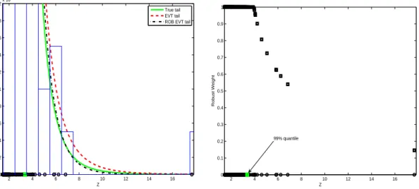
To illustrate this important point, we perform the following simple Monte Carlo experiment. We simulate 2,000 observations from a Student-t5 and fix the threshold at the 0.90 empirical quantile to
estimate the tail distribution. Left graph in Figure 1 shows estimation results. The classical EVT method clearly overestimates the whole tail distribution, which is highly affected by a few relatively
large observations that indeed do not fit well within the chosen parametric model. The robust EVT estimator introduced in equations (14) and (15) below produces a much better GPD estimate for the true tail distribution. This is illustrated also by the right graph in Figure 1, which presents the robust weight of each observation implied by this estimator. These weights automatically downweight the observations that are less well captured by the GPD tail. Intuitively, they identify some observations which are too influential in the score function (12) of the classical GPD estimator when compared to the other tail observations. Given that sgpd(x;ζ) is unbounded inx, these observations have a strong
impact on the classical EVT estimator, inflating the overall tail estimation. The robust EVT estimator is defined as follows. Given positive constantcgpd≥
√
2, robust estimator of GPD parameters, q, is defined by (Dupuis (1999))
EG∗[ψc(sgpd(X;q(G∗)))] = 0, (14)
where sgpd(x;ζ) is the GPD score function (12) and
ψc(sgpd(X;ζ)) := A(ζ) (sgpd(X;ζ)−τ(ζ))w(X;ζ),
w(X;ζ) := min(1, cgpd∥A(ζ) (sgpd(X;ζ)−τ(ζ))∥−1
)
. (15)
Matrix A(ζ) and vector τ(ζ) are solutions of the equations
Eζ0 [ ψc(sgpd(X;ζ0))ψc(sgpd(X;ζ0))⊤ ] = I Eζ0[ψc(sgpd(X;ζ0))] = 0.
Figure 1 shows that the robust estimator provides a nearly perfect tail estimation. This result is achieved by automatically down-weighting only a few outlying observations, using the weighting functionw(X;ζ) in (15); see right graph in Figure 1. Only observations above the 0.99 quantile are down-weighted, but the larger the tail observation, the lower the robust weight.5
The previous discussion is further supported by the following Monte Carlo simulation. We generate 1,000 samples of 2,000 IID observations each from a Student-t5 distribution, resembling model residual
distributions. Using different threshold levels, we estimate the 0.99 quantile of the t5-distribution
applying (i) the empirical quantile (HS), (ii) the Hill (1975) estimator, (iii) the classical EVT, and (iv) the robust EVT method. The simulation allows us to study the precision of quantile estimates and the sensitivity of classical and robust procedures with respect to threshold levels. The choice of threshold level plays a key role in EVT applications because it determines the trade-off between variance and bias of GPD parameter estimates.6 Figure 2 shows bias and mean square error (MSE) of
estimated 0.99 quantile for the four tail estimators, as a function of the chosen threshold level (number of observations in the tail). By definition, the empirical quantile does not depend on thresholds but is generally inaccurate. The Hill estimator is the most sensitive to the threshold level, making its empirical application rather delicate. The robust EVT method has the lowest MSE for most threshold levels, and outperforms classical EVT method consistently. For example, fixing the threshold at 0.90 quantile, i.e. using 200 tail observations, classical EVT quantile estimates have MSE 11% larger than robust estimates. For lower thresholds, i.e. using more tail observations, classical EVT estimates deteriorate rapidly, while robust EVT estimates are even more accurate in terms of MSE. Both in terms of bias and MSE, accuracy of robust EVT estimates is least sensitive to threshold levels among tail estimators. This is certainly a desirable property of robust EVT method because it is difficult to select thresholds optimally in empirical applications.7
In the following Monte Carlo experiments and empirical applications, we take the empirical 10th and 90th quantiles of model residual distributions as threshold levels for estimating lower and higher quantiles, i.e. using 200 tail observations. Such a threshold choice is the one suggested by McNeil and Frey (2000) for the classical EVT method and achieves a minimal MSE for this method in the Monte Carlo simulation of Figure 2. The lowest MSE of the robust EVT method is achieved at a lower threshold level; see Figure 2. Therefore, the VaR forecasting performance of robust EVT could be in principle further improved by considering different choices of the threshold level. We do not investigate this issue in more detail in the sequel.
1.5 Choice of Robustness Tuning Constants
The tuning constants c and cgpd in the estimating equations (5) and (14) control for the degree of
robustness of GARCH and GPD estimators, respectively. Following Mancini et al. (2005), we set such constants to achieve a given asymptotic efficiency under parametric reference models Pθ0 and Gζ0.
The relative efficiency of the robust estimatorais measured astrace(V(s; ˆθn))/trace(V(ψc; ˆθ¯n)), where V(s; ˆθn) and V(ψc; ˆθ¯n) are the asymptotic covariance matrices of the PML and robust estimators,
respectively. Relative efficiencies of robust estimators are presented in Mancini and Trojani (2010). For instance, the choice c = 11 implies approximately 98% asymptotic relative efficiency. The relative efficiency ofq is computed analogously.
2
Monte Carlo Simulation
PML GARCH Robust GARCH Empirical dist. fhs fhs rob
PML GPD evt —
Robust GPD — evt rob
The panel above summarizes the four VaR prediction methods studied here. For brevity, the method based on nonparametric residual bootstrap is called fhs. When GARCH dynamics are estimated using the robust estimator (5) we call this method fhs rob; evt rob uses robust estimators both for GARCH dynamics and GPD tail estimations; evt uses PML estimators at both stages. The simulation design allows to evaluate the contribution of each robustification step to the accuracy of VaR predictions. Comparing fhs and fhs rob VaR predictions allows to assess the potential improvement of VaR forecasts due to robust instead of PML estimation of the GARCH model. In Section 2.4 we compare VaR forecasts using true GARCH parameters. In that setting comparing evt and evt rob allows to assess the potential improvement of VaR forecasts due to robust instead of PML estimation of tail distributions.
We compute out-of-sample VaR forecasts at 1% and 5% confidence levels and horizons h = 1 day and h= 10 days, under an AR(1), asymmetric GARCH(1,1) model for daily returns. We simulate the following dynamics for Y :={Yt}t∈Z.
1. Student-t5 innovation model. In this experiment, innovation in model (1) is given by
Zt= ((ν−2)/ν)1/2Tν, (16)
where random variable Tν has a Student-t distribution with ν = 5 degrees of freedom. Hence Zt∼IID(0,1) and model (1) is dynamically correctly specified.
2. Laplace innovation model. Innovation in model (1) is given by
Zt= 2−1/2L, (17)
where random variableLhas a Laplace (or Double exponential) distribution. Such a distribution has a symmetric convex density and displays fatter tails than the t5-distribution. Also in this
experimentZt∼IID(0,1) and model (1) is dynamically correctly specified.
3. Replace-innovative model. In this model, Y :={Yt}t∈Z is generated as follows: Yt= ρ0+ρ1Yt−1+εt, with probability 1−κ, ˇ Yt, with probabilityκ, (18)
where ˇYt∼N(0, ϱ2), εt∼N(0, σ2t) and σt2 is given by (9). At timet there is a probabilityκ that
observation Yt is not generated by the GARCH dynamic. The possible “shock”, ˇYt, will affect
future realizations of the process mainly by “inflating” the conditional variance on subsequent days. In this experiment, model (1) is “slightly” misspecified as the dynamic equations (8)–(9) are not satisfied for every t. We set κ = 0.2% and ϱ = 10. The probability of contamination,
κ, is very low and implies (on average) 4 contaminated observations out of 2,000 observations. The choice for ϱ allows us to compare the accuracy of the different VaR estimators under very infrequent, but dramatic, (symmetric) shocks. Such shocks could occur over short time periods in real data, as for instance in daily equity returns.
We set the AR(1), asymmetric GARCH(1,1) model parameters toρ0 =ρ1= 0.01,α0 = 0.03,α1 = 0.02,
α2= 0.8, andα3 = 0.2. This parameter choice reflects somehow parameter estimates typically obtained
for daily percentage index or exchange rate returns; see for instance Bollerslev, Engle, and Nelson (1994). At the reference model Pθ0, annualized volatility of Yt is about 12%. The robust GARCH
estimators have tuning constantsc= 11. The robust GPD estimator hascgpd= 8. The sample sizeT =
2,000. Each model is simulated 1,000 times. For each simulated sample path, we use the VaR prediction methods (fhs, fhs rob, evt, evt rob) to compute VaR forecasts. In the financial industry, virtually only out-of-sample VaR forecasts are required and in-sample measurements of VaR are far less important. In our simulations and empirical applications all VaR forecasts are out-of-sample ones.
2.1 GARCH Dynamics Estimation
Bias and MSE of PML and robust estimators for the AR(1), asymmetric GARCH(1,1) model (8)–(9) are reported in Mancini and Trojani (2010). Estimation results for the robust estimator atrunc (with
l= 30 lags) discussed in Footnote 3 are also reported in the appendix. Under reference modelPθ0, i.e.,
when GARCH residuals are Gaussian, PMLE (which is indeed MLE) is only slightly more efficient than the robust estimators,aandatrunc. In all other experiments, both robust estimators always outperform
classical PML estimator in terms of mean square errors, especially under the replace-innovative model. The overall performances of the two robust estimators aand atrunc are very close butahas somewhat
lower mean square errors. The last finding supports the application of a for estimating GARCH-type models.
2.2 VaR Violation
Standard analysis of VaR prediction methods is based on violation tests. In the i-th simulation, a violation occurs when the actual loss is larger than the predicted VaR, i.e. I(i) := 1{yT,T+h(i) <
ˆ
yα
T,T+h(i)} = 1, and zero otherwise. Under the null hypothesis that VaR is correctly estimated, the
both horizons h = 1 day and 10 days. For α = 0.05 and 0.01 the expected number of violations are 50 and 10, and two-side confidence intervals at 95% level are [37,64] and [4,17], respectively. Table 2 shows number of violations for fhs, fhs rob, evt and evt rob. All methods exhibit numbers of violations within such confidence intervals, but it is known that violation tests have typically low power. Table 2 also hints some differences among VaR prediction methods. In the first two Monte Carlo experiments (Student-t5 and Laplace innovations), only evt rob never exhibits p-values below 0.10, even though
estimated GARCH models are correctly specified. These results suggest that evt rob can outperform other approaches even in setups relatively favorable to classical methods, but this phenomenon is not clearly detected by violation tests. Next section studies the precision of VaR forecasts, which is a key issue for measuring market risk.
2.3 Accuracy of VaR Prediction
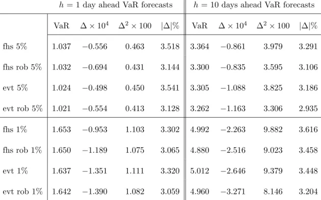
Left panel in Table 3 shows bias and MSE of one day ahead VaR predictions. In all Monte Carlo experiments, robust versions of FHS and EVT methods have smaller MSEs than corresponding classical versions. The reduction in MSE is small in the Laplace innovation model, but reaches about 80% in the contaminated replace-innovative model. In almost all cases, evt rob has the lowest MSE, often by several times. To gauge economic differences among VaR prediction methods we can compare nominal and effective coverage of predicted VaR. Under the Student-t5 model for example a $100 value portfolio
with µt = 0.01 and σt =
√
0.375 has a daily VaR at 1% of $2.05. If the true VaR is underestimated by $0.12, which is approximately one root MSE in the Student-t5 simulation (i.e. 0.12≈
√
0.015), the predicted VaR of $1.93 cannot attain the perfect coverage of 1% but is violated with a sufficiently close probability of 1.2%. Hence under this model all VaR prediction methods give economically sensible VaR predictions. Similar conclusions hold for the Laplace model. However, under replace-innovative model (18) underestimating the true VaR by $0.53 or $0.27, i.e. one root MSE of evt and evt rob methods, respectively, implies substantially different situations. In the evt case, predicted VaR at 1% is indeed violated with a probability of 6.8%, while in the evt rob case only with a probability of 2.8%,
and this difference is economically sizable. To further understand the magnitude of MSEs, we can standardize them by true unconditional variances. In the first two experiments, unconditional daily variance of percentage returns is 0.375. Hence a MSE of 0.015 for VaR at 1% level amounts to only 4% of the unconditional variance. Under replace-innovative model, MSEs of evt and evt rob are 49% and 12% of the unconditional variance (which is equal to 0.574), respectively, suggesting that evt rob provides much more accurate VaR predictions.
Right panel in Table 3 shows the accuracy of VaR predictions ath= 10 days ahead horizon. In the first two experiments the dynamic model (1) is correctly specified and all VaR prediction methods tend to perform similarly in predicting VaR at 5% level, although evt rob outperforms all other methods in predicting VaR at 1% level. In the third experiment the dynamic model (1) is slightly misspecified and both FHS methods perform very poorly, with fhs rob having the largest MSE for VaR predictions at 1% level. At first sight, the last finding might appear puzzling given the higher accuracy of robust GARCH estimates; see Mancini and Trojani (2010). This result is explained by the low breakdown point of VaR predictions based on nonparametric residual bootstrap.8 This point is discussed in Section 2.4 below.
In terms of MSE, evt rob largely outperforms all other methods. For example, under replace-innovative model the ratio of MSE of VaR forecasts at 1% level over 10-day unconditional variance is 69% for evt and 28% for evt rob, confirming that evt rob provides economically large improvements in VaR predictions.
2.4 Bootstrap Breakdown Point and Quantile Estimates Accuracy
To disentangle the contribution of nonparametric, PML and robust EVT tail estimation to VaR pre-dictions, we repeat the previous Monte Carlo simulation using true GARCH parameters. We also investigate theoretical predictions of equation (10) on breakdown points of bootstrap quantiles.
We estimate 5% and 1% quantiles (i.e. VaR) of ten days ahead return distribution. As GARCH parameters are not estimated, classical and robust FHS methods coincide and we call them “resampling” in this section. We consider different ways of implementing semiparametric bootstrap methods using
EVT. We make an additional distinction depending on whether the quantile of simulated ten days ahead distribution is estimated nonparametrically or using a GPD (PML or robust) estimator. This distinction highlights the additional contribution of parametric GPD over nonparametric tail estimations in producing accurate VaR forecasts. We compute VaR predictions using the following five methods:
1. Resampling (i.e. FHS method).
2. EVT applied to both daily returns and simulated ten days ahead returns.
3. Robust EVT applied to both daily returns and simulated ten days ahead returns.
4. EVT applied to daily returns, and empirical quantile of ten days ahead return distributions.
5. Robust EVT applied to daily returns, and empirical quantile of ten days ahead return distributions.
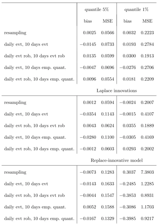
Table 4 reports simulation results for the five methods under the previous Monte Carlo experiments. All MSEs of VaR forecasts in Table 4 are lower than those in Table 3 as variability deriving from estimation of GARCH parameters is absent now. In the first two experiments (Student-t5 and Laplace innovations),
the data generating processes do not produce “outliers”. For 5% quantiles, resampling procedures and robust EVT perform well, but classical EVT method is the least precise. For 1% quantiles, robust EVT methods have uniformly higher accuracy. Therefore, the misspecification of the GPD tail in these Monte Carlo experiments produces a quite favorable trade-off for using our robust methods in estimating the true tail of GARCH residuals.
Under the replace-innovative model, resampling method breaks down in the estimation of 1% quan-tile, whereas it produces accurate results in estimating 5% quantile. From Table 1, the breakdown point of VaR at 5% level corresponds to 0.51% outliers in the data, whereas the breakdown point of VaR at 1% level is 0.10%. Hence as predicted by equation (10), κ= 0.20% of outliers in the data breaks down VaR predictions at 1%, but not at 5% using nonparametric residual bootstrap.9 For quantile at 1% level,
the ratio of MSE over 10-day unconditional variance is 129% for the resampling method (FHS), and only 16% for the robust EVT method applied to both daily and 10-day returns, confirming that robust
EVT provides economically large improvements in predicting VaR. Overall, robust EVT tail estimation is particulary important when forecasting VaR at low confidence levels and/or data are contaminated by outliers.
To further understand the impact of PML and robust GARCH estimates on VaR predictions, we repeated the Monte Carlo simulation but for comparison and to regularize the bootstrap procedure we always fitted the tails of daily innovation distributions (and 10-day ahead returns) with the classical EVT method. Unreported results confirm that VaR predictions based on robust GARCH estimates are still more accurate than VaR predictions based on PML GARCH estimates especially for the 10-day horizon and in presence of outlying observations. This finding suggests that robust GARCH estimates contributes significantly to the accuracy of VaR forecasts.
3
Real Data Estimation and Backtesting
We backtest VaR prediction methods on four historical series of daily rate of returns: S&P 500 index from December 1988 to July 2003, Dollar-Yen exchange rate from January 1986 to January 2005, Microsoft share price from March 1986 to January 2005, and Boeing share prices from January 1980 to January 2005. The data are downloaded from Datastream. Denote by y1, . . . , yN the historical series of
returns, where e.g.N = 4,500. To backtest for example evt rob method we proceed as follows. We use
n= 2,000 returns, i.e. about eight years of daily data, to estimate the AR(1), asymmetric GARCH(1,1) model with the robust estimator (5) and tuning constant c = 8. Return innovation distribution is estimated using the filtered return innovations, ˆz1, . . . ,zˆn, and the robust EVT approach discussed
in Section 1.4, with cgpd = 6 for robust GPD estimator (14).10 For day T = n, out-of-sample VaR
forecasts, ˆyαT ,T+h, are computed at horizons h = 1 day, 10 days, and confidence levels α = 1%, 5%,
using the semiparametric residual bootstrap discussed in Section 1.3. Left tail of simulated 10-day ahead return distribution is fitted using robust GPD estimator to calculate VaRs. The VaR prediction is calculated for each day T ∈ T = {n, n+ 1, . . . , N−h} using a moving time window of n historical
returns for filtering returns and estimating distributions. GARCH estimates, however, are updated only every 500 days. The other three VaR prediction methods are similarly backtested: fhs and fhs rob rely on nonparametric rather than semiparametric residual bootstrap; evt uses PML rather than robust GARCH estimation.
For comparison, we also include (i) Historical Simulation (HS); (ii) RiskMetrics (1995) (RM); (iii) Engle and Gonzalez-Rivera (1991) semiparametric GARCH model (EGR); (iv) Engle and Manganelli (2004) CAViaR model;11 and for 10-day ahead VaR predictions, (v) GARCH model applied directly to
10-day asset returns. The HS and RM methods are popular in financial industry. The EGR approach provides flexible and efficient estimates of semiparametric GARCH models. The CAViaR model offers a challenging benchmark for VaR predictions, which estimates VaR directly using quantile regressions.12
3.1 Data and GARCH Estimation
Table 5 shows summary statistics for the daily rate of returns. The different characteristics of assets make the backtesting exercise particularly interesting. For example, Dollar-Yen exchange rates have large skewness and Microsoft returns large kurtosis. PML and robust estimates of AR(1), asymmetric GARCH(1,1) models for the different financial assets are collected in Mancini and Trojani (2010). In several occasions and especially for the volatility parameters the two estimates are rather different. Next sections show how these estimates induce different VaR forecasts.
3.2 Backtesting VaR Prediction
To assess the forecasting performance of the VaR prediction methods we adopt the testing framework proposed by Christoffersen (1998). This framework consists of three tests and has become a standard setting for evaluating out-of-sample forecasts. We refer the reader to (Christoffersen 2003, Chapter 8) for an in-depth description of the tests; a short description is also available in Mancini and Trojani (2010). The test of unconditional coverage checks whether or not the overall number of violations is statistically acceptable. The test of independence aims at verifying possible clusterings of violations
over time. The test of conditional coverage checks in which respect the time series of VaR violations does not satisfy the correct conditional coverage.
Tables 6, 7 and 8 show number of violations and p-values of unconditional, independence and conditional coverage tests for one day ahead VaR forecasts.13 Only evt rob passes all violation tests
with p-values above 0.10. Nearly all other methods fail both unconditional and conditional coverage tests for the S&P 500 backtesting. For instance, in the conditional coverage test and VaR predictions at 5%, fhs has a p-value of 0.046, fhs rob of 0.076, EGR of 0.035, evt and CAViaR of 0.012, and HS below 0.001. Generally, HS and RM methods do not work well, especially for VaR predictions at 1% level with several p-values below 0.05. VaR prediction method based on semiparametric EGR model performs similarly to fhs method. The CAViaR model fails violation tests for the S&P 500 backtesting with most p-values below 0.05.
These empirical findings confirm the simulation results and document the accuracy of VaR pre-dictions based on our robust approach. We now turn the attention to the time series properties of VaR forecasts. Temporal profiles of VaR predictions have economic relevance because asset allocations need to satisfy VaR constraints and VaRs determine reserve amounts to cover market risk. Asset al-locations and reserve amounts cannot change heavily from one day to the next otherwise the financial firm can incur in a variety of costs, such as transaction costs or financial losses due to liquidation of risky assets at stressed prices in high volatile periods to reduce risk exposures. Left panel in Table 10 summarizes the time series properties of VaR forecasts for Dollar-Yen backtesting. The correspond-ing statistics for S&P 500, Microsoft and Boecorrespond-ing are similar and collected in Mancini and Trojani (2010). In Table 10 “VaR” denotes average VaR forecasts, ∆ average daily changes in VaR predictions
{yˆα
T+1,T+1+h−yˆT,Tα +h}T∈T, ∆2 corresponding empirical second moment, and |∆|% average absolute
relative changes in percentage. The last three statistics describe daily changes of VaR forecasts. In nearly all backtested time series and VaR confidence levels, evt rob has the lowest values of ∆2 and
Dollar-Yen backtesting, |∆|% for evt is 13% larger than those for evt rob. Using robust VaR predictions the financial firm can adjust portfolio risk exposures to VaR limits more smoothly and thus more efficiently. The empirical analysis of ten days ahead VaR forecasts confirms and further strengthens the previous findings. Table 9 shows number of violations of ten days ahead VaR forecasts and robust Newey and West (1987) two-side p-values for the null hypothesis that the given method predicts VaR correctly.14
The lowest p-value for evt rob is 0.28. All other FHS methods are too conservative in predicting VaR at 5% level for the Boeing backtesting, with p-values below 0.07. VaR prediction method denoted by
h-ret applies fhs method directly to non-overlapping 10 days returns. Henceh-ret avoids the resampling procedure to simulate daily returns up to 10 days horizon, and relies on the empirical quantile of estimated 10-day return innovations to predict VaR. CAViaR model is fitted to non-overlapping 10 days returns as well. Both methods do not work well. They suffer the inefficient use of available information, discarding 9 out of 10 observations when computing non-overlapping 10-day returns.15
RiskMetrics uses the suggested √h-rule to scale daily volatility to 10-day horizon but fails Microsoft backtesting with a p-value of 0.03. EGR fails Boeing backtesting with ap-value of 0.06.
In nearly all backtested time series, evt rob VaR forecasts are the most stable over time in terms of squared and absolute relative changes, ∆2 and |∆|%. For example, for VaR at 5% level, ∆2 for evt is 9% higher than that for evt rob in the Dollar-Yen backtesting; see right panel in Table 10. To save space descriptive statistics of HS, RM, EGR, CAViaR, andh-ret temporal VaR profiles are not reported but collected in Mancini and Trojani (2010). The h-ret and CAViaR methods have the most volatile temporal VaR profiles among all considered VaR prediction methods. EGR performs similarly as fhs method.
3.3 Tail Estimation Risk
An important source of variability of VaR forecasts can be re-estimation of tail distributions that occur every day, and induces the so-called tail estimation risk. Our Monte Carlo experiments suggest that under a number of realistic dynamic specifications, the VaR estimation risk implied by our robust
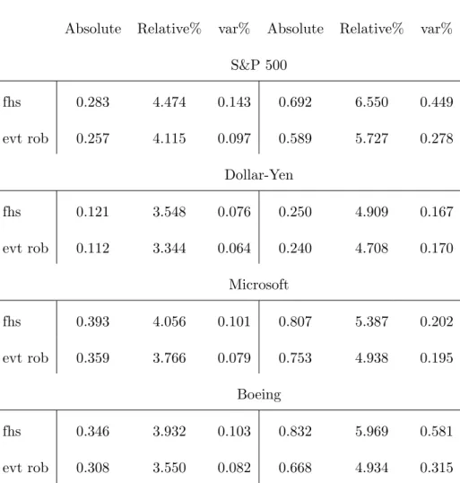
procedure is lower than the one of classical approaches. To measure such estimation risk exactly in real-data applications, we would need to compare predicted VaR and true VaR, but the latter is obviously unknown. A feasible approach to quantify estimation risk is to provide empirical prediction intervals for the VaR forecast itself. When a VaR prediction method is unbiased and behaves properly in terms of VaR violations, the narrower the prediction interval, the lower the tail estimation risk. Christoffersen and Gon¸calves (2005) propose a resampling technique to measure estimation risk and we follow their methodology here. As any other resampling techniques, the procedure is computationally demanding. To keep computations feasible, we limit the analysis toh= 10 days ahead VaR predictions based on fhs and evt rob. For both methods and for each dayT ∈ T, we obtainS= 199 VaR predictions{yˆT,Tα (s+)h}Ss=1 at confidence levels α = 5% and 1%, i.e. each day we repeat S times the forecasting procedures of classical FHS and robust EVT methods. The robust EVT method is particularly demanding because on each day and for each one of the 199 random samples, GPD distributions are fitted using the robust estimator to both tails of the GARCH residual distribution and to the left tail of simulated ten days ahead return distribution. For each day T ∈ T, we compute the prediction interval at 80% confidence level for the VaR forecast ˆyT,Tα +h,
[ Q0.1 ( {yˆT,Tα(s+)h}Ss=1 ) , Q0.9 ( {yˆT,Tα(s+)h}Ss=1 )] ,
where Qx(·) is thex-quantile of the empirical distribution of{yˆT,Tα (s+)h}Ss=1. Other confidence levels are certainly conceivable but the results based on the 80% level are likely to be representative of the findings based on other confidence levels.
Table 11 shows average absolute and relative widths of ten days ahead VaR prediction intervals in our backtesting period. For all backtested assets, evt rob has narrower prediction intervals than fhs, both in absolute and relative terms. Therefore, evt rob provides more accurate and reliable VaR predictions than fhs. For example, in S&P 500 and Boeing backtesting and for VaR forecasts at 1% level, classical FHS relative prediction intervals are 14% and 21% larger than those for robust EVT. In Table 11, var% denotes variance of daily changes in prediction intervals. In all but one case, daily
changes of evt rob have smaller variances than daily changes of fhs prediction intervals. In S&P 500 and Boeing backtesting and VaR forecasts at 1% level, such variances for evt rob are nearly 50% those of fhs. Overall, our robust procedure appears to control tail estimation risk in a better way than classical procedures and this induces more stable VaR profiles over time.
4
Conclusion
We propose a general robust semiparametric bootstrap method to estimate predictive distributions of GARCH-type models. Our approach is based on a robust estimation of parametric GARCH-type models and a robustified resampling method for GARCH residuals, which controls the bootstrap instability due to influential observations. In the latter, a robust extreme value estimator is used to fit innovation tail distributions above some threshold levels. A Monte Carlo study shows that the robust extreme value estimator provides more accurate quantile estimates and is less sensitive to the choice of threshold levels than classical estimators. Our robust procedure offers improvements in accuracy of VaR predictions, especially for several days ahead horizons and/or in presence of outlying observations. In nearly all Monte Carlo experiments, our robust procedure has lower mean square prediction errors than classical methods, often by a large extent. Only our method passes all validation tests at usual significance levels. Theoretical predictions of bootstrap breakdown points are confirmed by simulations and non robust bootstrap procedures break down approximately at the calculated breakdown point.
The simulation evidence is confirmed by the real data application. We backtest several VaR pre-diction methods using about twenty years of S&P 500, Dollar-Yen, Microsoft and Boeing daily returns. Only our robust procedure passes all validation tests at usual significance levels, and outperforms sev-eral other VaR prediction methods, such as RiskMetrics, CAViaR, Historical Simulation and classical FHS methods. Overall, robust VaR profiles are more accurate and more stable over time than classical forecasts. Given the accuracy of our robust method, the stability of VaR profiles is a desirable feature because it allows financial firms to adapt risky positions to VaR limits more smoothly and thus more
efficiently. We show empirically that our robust procedure controls for tail estimation risk better than classical methods and this induces more accurate and more stable over time VaR prediction intervals.
Robust semiparametric bootstrap methods have applications beyond risk management. For example, Engle and Gonzalez-Rivera (1991) propose an iterative procedure to estimate semiparametric GARCH models computing the likelihood function using nonparametric estimation of innovation distribution. Applying our robust procedure extends the estimation of such GARCH models to the robust setting. Another application of our method can be computing fund performance measures using the robust bootstrap procedure.
5
Funding
We gratefully acknowledge the financial support of the Swiss National Science Foundation (NCCR-FinRisk, Grants Nr. 101312-103781/1 and 100012-105745/1).
Notes
1For brevity equation (2) assumes a continuous profit and loss distribution.
2See e.g. Duffie and Pan (1997) and Gouri´eroux, Laurent, and Scaillet (2000) for a general discussion on conditional
VaR, and A¨ıt-Sahalia and Lo (2000) for an economic interpretation of VaR.
3
Formally, optimality results in Mancini et al. (2005) hold for ARCH- but not GARCH-type models. As in Sakata and White (1998), however, we can expect that our robust estimator performs well also under GARCH models with sufficient memory decay. To investigate this point, in the estimating function (4), we approximate the GARCH volatility by an ARCH model. For example in the GARCH(1,1) model,
σt2(θ) = α0+α1ε2t−1(θ) +α2σt2−1(θ) = +∞ ∑ j=0 αj2(α0+α1ε2t−1−j(θ) ) = l−1 ∑ j=0 αj2 ( α0+α1ε2t−1−j(θ) ) +αl2σ 2 t−l(θ) =:σ 2 t(θ)trunc+αl2σ 2 t−l(θ)≈σ 2 t(θ)trunc.
For sufficiently large lagl,αl2σ2t−l(θ)≈0, and the bias of the robust estimatoratruncbased onσ2t(θ)truncis expected to be negligible. Monte Carlo simulation in Section 2.1 studies this issue.
4
The terminology leverage effect was introduced by Black (1976) who suggested that a large negative return increases the financial and operating leverage, and rises equity return volatility; see also Christie (1982). Campbell and Hentschel (1992) suggested an alternative explanation based on the market risk premium and volatility feedback effects; see also Bekaert and Wu (2000). Following common practice, we shall use the terminology leverage effect when referring to the asymmetric reaction of volatility to positive and negative return innovations.
5
Several authors have emphasized the instability of PML estimates of GPD when a moderate number of influential points is present in the sample; see for instance Cowell and Victoria-Feser (1996) and Ju´arez and Schucany (2004).
6
A too high threshold results in too few exceedances and hence high variance estimators. A too low threshold induces biased estimates as the approximation implied by limit result in equation (13) cam imply large errors.
7
See McNeil and Frey (2000) and Gonzalo and Olmo (2004) for further evidence on the choice of the threshold level.
8
To raise the breakdown point of nonparametric bootstrap quantiles, Singh (1998) suggests to winsorize the data before bootstrapping. We winsorized innovations at 0.5% and 1% levels, respectively, and then we computed ten days ahead VaR predictions using fhs and fhs rob. MSEs of the winsorized VaR predictions did decrease but only by a small amount and the results are not reported.
9
This finding also appears in the right panel of Table 3.
10
Considering the “noisier” nature of real data, as opposed to simulated data, and the different characteristics of financial time series (indexes, stocks and exchange rates) used in backtesting, we take a somewhat more conservative viewpoint setting the robustness tuning constantscandcgpdto lower levels than in the Monte Carlo study.
11
Engle and Manganelli (2004) find that empirically Asymmetric Slope and Indirect GARCH CAViaR models tend to out-perform other CAViaR specifications. Given the asymmetric impact of positive and negative returns on volatility (and pos-sibly on quantiles) documented in our sample, we use the Asymmetric Slope CAViaR model in our empirical analysis. The Matlab code for the CAViaR model is freely available at Simone Manganelli’s webpage,http://www.simonemanganelli.org.
12Koenker and Bassett (1978) introduce quantile regression methods; see also Foresi and Peracchi (1995) and Peracchi
(2002). From a robustness perspective, drawbacks of quantile regression is its behavior under heteroscedasticity and the non robustness to leverage points; see Koenker and Bassett (1982).
13
See also Kuester, Mittnik, and Paolella (2006) for a recent comparison of FHS methods.
14
Robust standard errors are computed using Newey–West covariance matrix withh−1 lags.
15
In principle, EVT methods could be applied directly to 10 days returns as well, but then the issue of limited sample size would be even more sever. To achieve 200 data points as in our previous applications, 80 years of daily returns would be required.