BRNO UNIVERSITY OF TECHNOLOGY
VYSOKÉ UČENÍ TECHNICKÉ V BRNĚFACULTY OF INFORMATION TECHNOLOGY
DEPARTMENT OF COMPUTER GRAPHICS
AND MULTIMEDIA
FAKULTA INFORMAČNÍCH TECHNOLOGIÍ ÚSTAV POČÍTAČOVÉ GRAFIKY A MULTIMÉDIÍ
ACTIVITY OF NEURAL NETWORK IN HIDDEN LAYERS –
VISUALISATION AND ANALYSIS
ZOBRAZENÍ A ANALÝZA AKTIVIT NEURONOVÉ SÍTĚ VE SKRYTÝCH VRSTVÁCH
MASTER’S THESIS
DIPLOMOVÁ PRÁCEAUTHOR
Bc. MARKO FÁBRY
AUTOR PRÁCE
SUPERVISOR
Ing. MARTIN KARAFIÁT, Ph.D.
VEDOUCÍ PRÁCE
Abstract
Goal of this work was to create system capable of visualisation of activation function values, which were produced by neurons placed in hidden layers of neural networks used for speech recognition. In this work are also described experiments comparing methods for visualisation, visualisations of neural networks with different architectures and neural networks trained with different types of input data. Visualisation system implemented in this work is based on previous work of Mr. Khe Chai Sim and extended with new methods of data normalization. Kaldi toolkit was used for neural network training data preparation. CNTK framework was used for neural network training. Core of this work — the visualisation system was implemented in scripting language Python.
Abstrakt
Cílem této práce je vytvořit systém schopný zobrazení hodnot aktivačních funkcí neuronů nacházejících se v skrytých vrstvách neuronových sítí použitých na rozpoznávání řeči. Dále byly na tomto systému provedeny experimenty porovnávající vizualizační metody, vizualizace neuronových sítí s různými architekturami a s různými druhy vstupních dat. Vizualizační systém implementovaný v rámci této práce je založen na předchozí práci pana Khe Chai Sim a rozšířen o nové způsoby normalizace vstupních dat. Pro přípravu trénovacích dat neuronových sítí byl použit framework Kaldi. Pro samotné trénování neuronových sítí byl použit nový framework CNTK. Jádro práce — samotný vizualizační systém byl implementován v skriptovacím jazyce Python.
Keywords
deep neural network, hidden layer, speech recognition, visualisation, analysis, activations, t–SNE, Kaldi, CNTK
Klíčová slova
hluboká neuronová síť, skrytá vrstva, rozpoznávání řeči, vizualizace, analýza, aktivace, t–SNE, Kaldi, CNTK
Reference
FÁBRY, Marko. Activity of Neural Network in Hidden Layers – Visualisation and Analysis. Brno, 2016. Master’s thesis. Brno University of Technology, Faculty of
Activity of Neural Network in Hidden Layers –
Visualisation and Analysis
Declaration
Hereby I declare that this master’s thesis was prepared as an original author’s work under the supervision of Ing. Martin Karafiát Ph.D. All the relevant information sources, which were used during preparation of this thesis, are properly cited and included in the list of references.
. . . . Marko Fábry 25th May 2016
Acknowledgements
I would like to thank to Ing. Martin Karafiát, Ph.D., for his professional help and especially for encouraging me in difficult times. I would also like to thank to my friends and family, for mentally and materialy supporting me while I was writing this thesis.
I also greatly appreciate access to computing and storage facilities owned by parties and projects contributing to the National Grid Infrastructure MetaCentrum provided under the programme ”Projects of Projects of Large Research, Development, and Innovations Infrastructures“ (CESNET LM2015042).
c
○ Marko Fábry, 2016.
This thesis was created as a school work at the Brno University of Technology, Faculty of Information Technology. The thesis is protected by copyright law and its use without author’s explicit consent is illegal, except for cases defined by law.
Contents
1 Introduction 3 2 Neural networks 4 2.1 Biological neuron . . . 4 2.2 Artificial neuron . . . 5 2.2.1 General model . . . 5 2.2.2 Types of units . . . 5 2.3 Neural Network . . . 72.3.1 Deep Neural Network . . . 8
2.3.2 Softmax output layer. . . 8
2.4 Learning. . . 8
2.4.1 Error function . . . 9
2.4.2 Gradient descent . . . 9
2.4.3 Backpropagation . . . 10
2.5 Specific types of Neural Networks . . . 11
2.5.1 Bottleneck Neural Networks . . . 11
2.5.2 Recurrent Neural Networks . . . 11
2.5.3 Long Short-Term Memory Neural Networks . . . 12
3 Automatic Speech Recognition 13 3.1 Automatic speech recognition system . . . 13
3.1.1 Feature extraction . . . 13
3.1.2 Acoustic modelling . . . 14
3.1.3 Acoustic matching . . . 14
3.1.4 Language model . . . 14
3.1.5 Speech decoding . . . 14
3.2 Deep Neural Networks in ASR . . . 15
4 High dimensional data projection 16 4.1 Dimension reduction . . . 16
4.2 Stochastic Neighbour Embedding (SNE) . . . 16
4.3 Crowding problem . . . 17
4.4 t-Distributed Stochastic Neighbour Embedding (t-SNE) . . . 17
5 Implementation of visualisation system 19 5.1 Data preparation . . . 19
5.2 Neural Network training . . . 19
5.3 Activation extraction. . . 20
5.4 Activation visualization . . . 20
5.4.1 Activity vectors. . . 21
5.4.2 Normalised entropy . . . 21
5.4.3 Hidden activity space . . . 22
5.4.4 Delaunay triangulation. . . 23
5.4.5 Ranking vectors . . . 24
5.4.6 Interpretable activity regions . . . 24
5.4.7 Interpretable regions in 3D . . . 26
5.4.8 Activity visualisation. . . 26
6 Experiments 28 6.1 Dataset description . . . 28
6.2 Compensating dataset statistical characteristics . . . 29
6.2.1 Attribute occurrence normalisation . . . 29
6.2.2 Silence trimming . . . 29
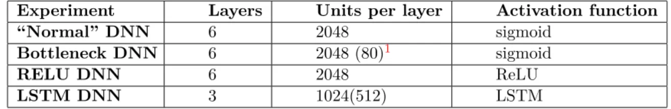
6.3 Experimental set-ups . . . 30
6.3.1 Experimental architectures . . . 30
6.3.2 Experimental environments . . . 30
6.4 Performance of the analysed networks . . . 31
6.5 Comparison of different views on experimental data . . . 32
6.6 Comparison of visualisation methods . . . 35
6.7 Analysis of NNs with different architectures . . . 37
6.8 Analysis of NNs trained with different datasets . . . 40
6.9 Experiments epilogue. . . 41
7 Conclusion and future plans 42 Bibliography 44 Appendices 46 List of Appendices . . . 47
A Contents of DVD 48 B Example scripts for CNTK 49 B.1 Activation printing script . . . 49
Chapter 1
Introduction
Current state of the art methods in Automatic Speech Recognition and in many other fields, for example computer vision, stock market prediction or scheduling optimization are using artificial neural networks.
Artificial neural networks are mathematical models inspired by principles of biological nervous systems, in particular human brain. Although neural networks are widely and frequently used and their models and learning algorithms are mathematically well defined, they are used essentially as black boxes, without much understanding of their
inner workings. Reason behind this is that practically used neural networks have large number of learnable parameters, therefore their structure easily becomes very complex.
This thesis is mainly based on the work of Khe Chai Sim and it aims to recreate and extend experiments described in his recent article [16]. Motivation for this work is in visualisation of artificial neuron activations in similar fashion to methods used in human brain research, like positron emission tomography (PET) scan, which shows how the human brain and its parts are working.
First part of this text provides basic theoretical knowledge and overview of technologies used in current research of neural networks and automatic speech recognition. This part of the thesis was done in the therm project. The second part describes implementation of system capable of visualising different neural network architectures. Subsequently, experiments performed using this system on selected architectures are described and analysed.
This work is segmented in chapters as follows. Chapter 2 — Neural networks
describes basic structural units and learning principles of neural networks. There are also described particular types of neural networks used later in experimental part of this work. Chapter 3 — Automatic Speech Recognition deals with the usage of neural
networks in automatic speech recognition. In chapter 4 — High dimensional data projection are provided basic informations about the Stochastic Neighbour Embedding,
method selected for high-dimensional data visualization. Chapter 5 — Implementation
of visualisation system describes implemented system for experiments on neural
networks and their usage in speech recognition. This system covers conversion of sound files to acoustic features, training neural network on these features, printing the activation values of hidden layers of the neural network and — the main concern of this work — visualizing the result. Consequently, multiple experiments conducted with different types of neural networks are described in chapter 6 — Experiments.
Finally, chapter 7 — Conclusion and future plans contains overall review of this
Chapter 2
Neural networks
This chapter explains origins and basic principles of neurons, neural networks and learning. Content of this chapter is mainly based on publication [2], unless otherwise stated.
2.1
Biological neuron
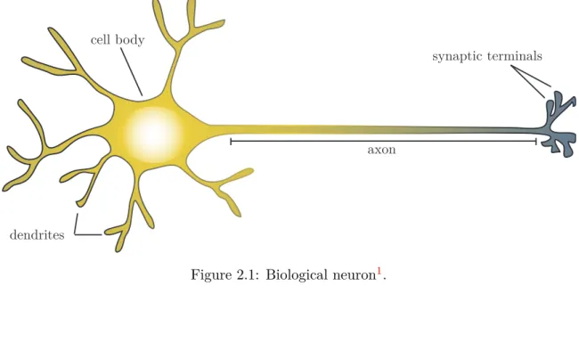
Biological neuron (see figure 2.1) consists of main body named soma, which has many “input” endings called dendrites and one very long projection – axon, which splits into
multiplesynaptic terminals. Synaptic terminals are “output” endings of neuron connected
to dendrites of other neurons. Neuron “fires”, when there is sufficient amount of electrical impulses from neuron’s dendrites that is greater than threshold. It means that the neuron propagates electrical signal through his axon and synaptic terminals to following connected neurons. The neuron becomes numb for a short period of time after propagation.
cell body
axon
synaptic terminals
dendrites
Figure 2.1: Biological neuron1.
1
2.2
Artificial neuron
2.2.1 General model
An artificial neuron or neural network unit is basic building block of neural networks. It
transforms vector of inputsx= (𝑥1, 𝑥2, ..., 𝑥𝑑) to single output yusing composition of two
functions:
1. Anet value function 𝜉, which computesnet value 𝜐using neurons inputsxand their respective weightsw:
𝜐=𝜉(𝑥, 𝑤) (2.1)
Mostly weighted sum or some kind of a vector distance function is used. 2. An activation function 𝜑, which computes neurons output yusing net value 𝜐:
𝑦 =𝜑(𝜐) (2.2)
Resulting output value is then copied to all following neurons. There are many types of activation functions. The most used, with regards to speech recognition, will be described in following sections.
Artificial neuron was inspired by the biological neuron. The similarity between artificial and biological neurons can be seen in previous function definitions. The net value function aggregates weighted input values, like biological neuron aggregates electrical impulses. Consequently, according to this net value, activation function decides intensity, with which the neuron will fire (or inhibit input signals).
2.2.2 Types of units
Because of many possible combination of suitable net value and activation functions, there are multiple types of neural network units. In following sections are briefly described important currently used units. Content of this section is inspired by the book [2].
Linear threshold unit
Linear threshold unit is sometimes incorrectly called perceptron, after single layer neural
network in which it was originally used. It is considered to be first artificial neuron. Perceptron was designed by Frank Rosenblatt in 1957 [13], based on mathematical model provided by McCulloch and Pitts [10].
Linear threshold unit uses linear net value function:
𝜐=
𝑚
∑︁
𝑖
(𝑤𝑖*𝑥𝑖) (2.3)
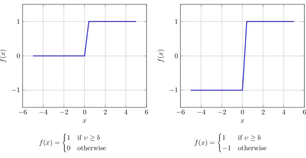
The step function (see figure 2.2a) or the sign function (see figure 2.2b) is used as the activation function. Output of the unit depends on its property 𝑏 called bias. Bias is
negative threshold independent of any input variables. When weighted sum of inputs is greater than |𝑏|, linear threshold unit produces value 1 on its output - the neuron fires, otherwise it produces 0 (for step function) or−1 (for sign function) - it inhibits inputs.
−6 −4 −2 0 2 4 6 −1 0 1 𝑥 𝑓 ( 𝑥 ) 𝑓(𝑥) = {︃ 1 if𝜐≥𝑏 0 otherwise
(a) Step activation function (for bias𝑏= 0).
−6 −4 −2 0 2 4 6 −1 0 1 𝑥 𝑓 ( 𝑥 ) 𝑓(𝑥) = {︃ 1 if𝜐≥𝑏 −1 otherwise
(b) Sign activation function (for bias 𝑏= 0). Figure 2.2: Activation functions of linear threshold unit.
Sigmoid unit
Sigmoid neuron uses same net value function as the linear threshold unit - weighted sum
of inputs. Sigmoid function (sometimes called logistic function) is used as the activation
function (see figure2.3a). This function has the output in range (0; 1), which is suitable for representing probabilities of classified samples to belong to certain class. Other alternative is hyperbolic tangent function (see figure2.3b). Both functions have continuous output range. It enables them to be used in neural networks that are using some variation of gradient descent learning described later in text.
−6 −4 −2 0 2 4 6 −1 0 1 𝑥 𝑓 ( 𝑥 ) 𝑓(𝑥) = 1 (1 +𝑒−𝑥)
(a) Sigmoid function.
−6 −4 −2 0 2 4 6 −1 0 1 𝑥 𝑓 ( 𝑥 ) 𝑓(𝑥) = tanh(𝑥)
(b) Hyperbolic tangent function. Figure 2.3: Activation functions of sigmoid unit.
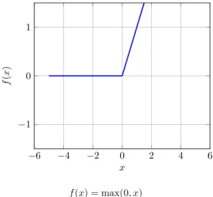
Rectified linear unit (ReLU)
Rectified linear unit (ReLU) uses linear net value function similarly to functions described
above. Rectified linear function is used as the activation function (see figure 2.4). These units are becoming more popular than the sigmoid ones, because they have far lower computational complexity - practically only instruction needed comparison with zero.
−6 −4 −2 0 2 4 6 −1 0 1 𝑥 𝑓 ( 𝑥 ) 𝑓(𝑥) = max(0, 𝑥)
Figure 2.4: Activation function of rectified linear unit.
2.3
Neural Network
Neural Networks (NNs) are considered as universal functions approximators from the
mathematical point of view. Given the sufficient number of parameters, neural networks can approximate any given vector space mapping, therefore NNs should be capable of performing any classification task. The most basic type of neural network is
feed-forward neural network. It is acyclic oriented graph with one output layer and at
least onehidden layer. Nodes in these layers are neurons and edges are outputs of neurons
of the previous layer and at the same time inputs to neurons of the next layer [8]. Every edge has assigned its respective weight. There is convention, that inputs are also considered as layer, even though this input layer contains no neurons. Example
𝑖1 𝑖2 𝑖3 𝑖4 𝑜1 𝑜2 𝑜3
Input layer 1. Hidden layer 2. Hidden layer Output layer Figure 2.5: Neural network example.
[Inspired byhttp://www.texample.net/tikz/examples/neural-network/.]
2.3.1 Deep Neural Network
Deep Neural Networks (DNNs) is designation for neural network that has several hidden
layers (often containing multiple different types of units), as opposed to shallow neural network, which has usually only one hidden layer [5].
2.3.2 Softmax output layer
For multi-class classification tasks, it is usually desirable to normalize neural network classification results. Softmax function (see equation (2.4)) is usually used for this
purpose. It normalizes the 𝑗−𝑡ℎ neuron’s output, with respect to all outputs of neurons 𝑥0, 𝑥1, ..., 𝑥𝑘 in output layer. Softmax output layer is different from previously mentioned
feed forward layers, because its neurons are fully interconnected.
𝑝𝑗 = 𝑒𝑥𝑗 ∑︀ 𝑘 (𝑒𝑥𝑘) (2.4)
2.4
Learning
Learning in biological neural networks is based on strengthening of the synapses which are connections between neurons. In artificial neural networks, these connections are represented with weights of unit inputs. Because learning can be defined as making less mistakes in given task, the amount of weights which are strengthened (or weakened) is based on number of correctly (or incorrectly) classified samples. Content of this section originates in publications [2, 8, 5]. Content of section 2.4.3 is mainly inspired by publications [17,11].
2.4.1 Error function
Error function ℰ(w) is function that represents quality of neural network. It is used in learning with teacher to determine ratio of incorrect outputs. The main goal of learning is to minimize this objective function. It is defined in equation (2.5), as expectation of error metric 𝐸(w;x), between desired output vector t = (𝑡1, 𝑡2, ..., 𝑡𝑛) and real neural
network output vectoro= (𝑜1, 𝑜2, ..., 𝑜𝑛) for given input vectorx= (𝑥1, 𝑥2, ..., 𝑥𝑚).
ℰ(w) = 1
𝑁
∑︁
𝑥∈𝑋
𝐸(x;w) (2.5)
Currently, two of the most used examples of error metrics are Mean Square Error
(MSE) (see equation (2.6)) andCross-Entropy (CE) (see equation (2.7)). The MSE metric
is mainly used in pattern learning applications, whereas the CE metric is mostly used in classification tasks. 𝐸𝑀 𝑆𝐸(x;w) = 𝐾 ∑︁ 𝑘=0 (𝑜𝑘−𝑡𝑘)2 (2.6) 𝐸𝐶𝐸(x;w) =− 𝐾 ∑︁ 𝑘=1 𝑡𝑘ln(𝑜𝑘) (2.7) 2.4.2 Gradient descent
Gradient descentis an algorithm for minimization of functions with multiple input variables.
The main idea behind gradient descent is to initialize input variables to random values at the start and keep changing them until we reach point where difference between two consequent output values are acceptably small. Values are changed in respect to negativegradientwhich
is the vector of first derivations of the minimized function (see equation (2.8)). Condition to gradient descent method is, that it requires function to be defined and differentiable for all possible input variables in order to find the derivatives.
∇𝑓(𝑥) = [︂𝜕𝑓 𝜕𝑥1, 𝜕𝑓 𝜕𝑥2, ... , 𝜕𝑓 𝜕𝑥𝑛 ]︂𝑇 (2.8) One step of the gradient descent algorithm can be represented with equation (2.9):
𝑥(𝑡+ 1) =𝑥(𝑡)−𝜇∇𝑓(𝑥(𝑡)), (2.9)
where𝑥(𝑡) is the vector of inputs in current step𝑡of the algorithm,∇𝑓(𝑥(𝑡)) is gradient
of function 𝑓 in point 𝑥(𝑡), 𝜇 is learning coefficient and 𝑥(𝑡+ 1) is the resulting vector
of inputs.
Learning coefficient𝜇representsstep sizeof the algorithm. If it is too small, the learning
is too slow. On the other hand, if it is too big, it is possible, that the algorithm misses the desired minimum. The fact that learning coefficient can vary between steps is often used in methods determining suitable learning coefficient dynamically [5].
Disadvantage of gradient descent is, that for non-convex functions the algorithm can get stuck in local minimums. Another disadvantage is that the resulting minimum is dependent on selection of starting points.
For large training sets, it is usually more convenient to generate so called mini-batches
— batches of randomly selected training vectors, which represent whole training set. During learning phase, weights are not updated after every training vector but after every mini-batch and average gradient computed of the mini-mini-batch is used for the update. This method speeds up the learning process and it is calledstochastic gradient descent (SGD) [5].
2.4.3 Backpropagation
Learning in DNNs consists of two phases:
1. Forward phase: The neural network inputs are in this phase propagated forward,
as they would in the case of classification. Output values of the classification are compared to expected values and an error valueis computed based on chosen error metric.
2. Backpropagation phase: Error values are propagated in backward direction from
outputs to inputs throughout the network layers. The gradients at the previous layers are learned as a function of the errors and weights in the layer ahead.
Every weight of nodes in neural network is updated according to equation (2.10), which is clearly based on gradient descent method described in section 2.4.2. If the minimized function is error metric 𝐸 and its input is vector wji, it can be deduced:
Δ(𝑙)𝑤 𝑗𝑖 =−𝜇 𝜕𝐸 𝜕 (𝑙)𝑤 𝑗𝑖 Δ(𝑙)𝑤 𝑗𝑖 =−𝜇 𝜕𝐸 𝜕 (𝑙)𝜐 𝑗 𝜕 (𝑙)𝜐𝑗 𝜕 (𝑙)𝑤 𝑗𝑖 Δ(𝑙)𝑤 𝑗𝑖 =−𝜇 𝜕𝐸 𝜕 (𝑙)𝑦 𝑗 𝜕 (𝑙)𝑦𝑗 𝜕 (𝑙)𝜐 𝑗 𝜕 (𝑙)𝜐𝑗 𝜕 (𝑙)𝑤 𝑗𝑖 Δ(𝑙)𝑤 𝑗𝑖 =𝜇(𝑙)𝛿𝑗 (𝑙)𝑥𝑖 (2.10) where: (𝑙)𝛿 𝑗 =− 𝜕𝐸 𝜕 (𝑙)𝑦 𝑗 𝜕 (𝑙)𝑦 𝑗 𝜕 (𝑙)𝜐 𝑗 (2.11) and: (𝑙)𝑥 𝑖 = 𝜕 (𝑙)𝜐𝑗 𝜕 (𝑙)𝑤 𝑗𝑖
(note: see equation (2.1)) (2.12) where Δ (𝑙)𝑤
𝑗𝑖 is the error derivative - value by which the 𝑖−𝑡ℎ input of the 𝑗−𝑡ℎ
neuron in layer 𝑙 will be updated, (l)x is the input vector of layer 𝑙, (l)y is the output vector of layer𝑙,𝜇 is the learning rate, (𝑙)𝜐𝑗 is the net value of the 𝑗−𝑡ℎ neuron in layer𝑙
and (𝑙)𝛿
𝑗 which is the derivation of error metric and activation function and it is typically
called the credit of the neuron.
Backpropagation starts in the output layer 𝐿, where the error derivative Δ (𝐿)𝑤𝑗𝑖
𝑦 ( 𝜕𝐸
𝜕 (𝐿)𝑦
𝑗) and the output of the activation function 𝑦 with respect to output
of the net value function 𝜐 (𝜕 (𝐿)𝑦𝑗
𝜕 (𝐿)𝜐
𝑗), multiplied by inputs
(L)x
i and learning rate 𝜇
(see equation (2.13)). Δ(𝐿)𝑤 𝑗𝑖 =𝜇 𝜕𝐸 𝜕 (𝐿)𝑦 𝑗 𝜕 (𝐿)𝑦𝑗 𝜕 (𝐿)𝜐 𝑗 (𝐿)𝑥 𝑖 (2.13)
In every hidden layeris the error derivative computed asweighted sum of credits of the following layer with respect to the total inputs to the units in layer above (𝑙+1)𝛿
𝑗,
multiplied bythe output of the activation function𝑦with respect to output of the net value function𝜐of the current layer (𝜕 (𝑙)𝑦𝑗
𝜕 (𝑙)𝜐
𝑗), multiplied by inputs
(l)x
iand learning
rate 𝜇(see equation (2.14)).
Δ(𝑙)𝑤 𝑗𝑖=𝜇 𝑛 ∑︁ 𝑘=1 ( (𝑙+1)𝑤 𝑘𝑗 (𝑙+1)𝛿𝑗) 𝜕 (𝑙)𝑦 𝑗 𝜕 (𝑙)𝜐 𝑗 (𝑙)𝑥 𝑖 (2.14)
2.5
Specific types of Neural Networks
This section introduces some of the many specific architectures of neural networks, that are currently researched and used for their particular abilities. Content of this section is inspired by articles [8,7,4].
2.5.1 Bottleneck Neural Networks
Bottleneck NNs have at least one hidden layer called bottleneck (BN) with significantly
smaller number of units than hidden layers before and after this layer. This results in compression of the information flowing through the bottleneck layer. Since the information is forced to be compressed, the neural network learns to discard unnecessary information and compress useful information. Systems based on bottleneck NNs are generally slightly more resilient against noised data. They are also less prone to the over-fitting problem, which in simple terms means, that the neural network is unable to generalize - to classify different data than it was trained on. Bottleneck NNs are often used for noise removal and compression in image or audio precessing tasks and feature extraction.
2.5.2 Recurrent Neural Networks
Recurrent Neural Networks (RNNs) are different than standard feed-forward DNNs
described in section 2.3, because they allow creating cycles in their topology. This fact allows RNNs to efficiently model sequential processes. The cycle creates feedback connection in neural network, which provides for the RNNs the ability to predict following input values from the previous input values of the sequence. This ability is especially useful in tasks where output does not depend solely on current input value but on arbitrary number of previous values like speech or language. For simplicity, the RNN can be viewed as standard feed forward NN, with added memory cells, which store the internal state of the neural network units. When plain RNNs are trained using modified version of back-propagation algorithm (Back Propagation Through Time (BPTT)), they
fact that when trained, one layer of RNN units can by unfolded as 𝑡 layers of standard
feed-forward DNN, where 𝑡 is count of all inputs 𝑥𝑡′ up to current input 𝑥𝑡. In such
extremely deep neural network the gradient can easily fade away or start exponentially growing. Currently there exist many modifications of RNN neural networks, but this work concerns only with the most popular type - the Long Short Term Memory NN, which does not suffer from vanishing - exploding gradient problem.
2.5.3 Long Short-Term Memory Neural Networks
Long Short-Term Memory (LSTM) neural network is a subtype of Recurrent Neural
Networks suggested by Hochreiter and Schmidhuber in [7]. LSTM neural networks are composed of complex neural units called memory blocks. These blocks with feedback loops
are able to store network state information in small memory called memory cell.
Information flow of memory block is controlled by three standard sigmoid neural units called gates. Theinput gate controls amount of information able to enter the LSTM unit.
Similarly, the output gate controls amount of information proceeding to the next layer
of the LSTM network. The last gate – forget gate enables the memory block to discard
information stored in memory cell, which enables the LSTM network to dynamically adapt to continuous input streams.
As stated above, all these gates are sigmoid units, which have their own weight matrices capable of learning and activation functions determining the amount of information to input, forget or output. Action of the gate is implemented as point-wise multiplication of the gate value and the respective input which gate controls. This effectively solves vanishing / exploding gradient problem from which suffer the RNNs, because the activation functions of the gates, especially the forget gate, prevent the gradient from decreasing / increasing uncontrollably.
It is necessary to note that the input to the LSTM unit before it reaches the input gate is squashed into range (−1; 1) with the tanh function. The output of the memory before
reaching the output gate is also adjusted with thetanh function to range (−1; 1).
Some practical implementations of LSTM NNs are employing several times more memory cells while maintaining the computational complexity by using special projection layers. These projection layers are reducing the number of recurrent outputs of memory cells. In this way there are more units for data processing, but less recurrent outputs which reduces learning time. This approach is described in more detail in article [15].
This section provided only very brief introduction to the currently popular LSTM neural networks. For more detailed informations about LSTM NNs and their abilities, please see articles [7,4,14].
Chapter 3
Automatic Speech Recognition
An Automatic Speech Recognition (ASR) is a system that converts the speech signal into
words. Such systems are used to control digital devices with simple commands or data entering in mobile devices. Current state-of-the-art ASR systems are providing great results on simple tasks, such as recognition of isolated words or read speech. Some practical applications are already usable, but there is still more research needed to improve their performance. Contents of this chapter are inspired by publications [18,5].
3.1
Automatic speech recognition system
Basic scheme of Automatic Speech Recognition system is depicted in figure3.1. Functions of individual blocks will be briefly described in following sections.
speech text
feature
extraction accousticmatching decoding
language model accoustic models or patterns
Figure 3.1: Automatic speech recognition system [18].
3.1.1 Feature extraction
The first thing that is needed in order to create speech recognition system, is to extract speech coefficients, sometimes also called features, from the input speech recordings. This
is done by filtering out unnecessary components of speech signal like DC offset, mean value or pitch to unify the speech and to limit the data to reasonable size. Consequently, the speech is split into smaller overlapping parts called frames, in which the speech signal
should be relatively stationary. Frames are commonly processed by the spectral or linear prediction analysis to compute the Mel Frequency Cepstral Coefficient (MFCC) or the Linear Predictive Coefficients (LPC) respectively. Vectors of these coefficients are the
previously mentioned features. DNNs used for speech recognition are usually trained using
filter-bank (sometimes called “f-bank”) features. These features are created from frames
by Discrete Fourier Transformation (DCT) and by using bank of filters with usually 41
coefficients (including energy) distributed on a log mel-scale [18].
3.1.2 Acoustic modelling
Acoustic modelling in speech recognition systems often utilized Gaussian Mixture Models (GMM) which are predicting posterior probabilities of Hidden Markov Model (HMM)
states. In other words, in every state of HMM is statistical distribution represented by mixture of diagonal covariance Gaussians (the GMM), which returns a likelihood for a vector of features. Acoustic model consists of many individual HMMs, each representing one basic acoustic unit – phoneme (sometimes also called phone). Since phonemes are
context dependent, current systems usually use triplets of phonemes - triphones. In the
triphone, every individual phoneme is in triplet with preceding and following phoneme. This extends number of possible output classes, but it significantly improves overall speech recognition results.
3.1.3 Acoustic matching
Acoustic matching is the process of scoring incoming feature vectors with individual HMM
models. Problem of acoustic matching is spatial and temporal variability. Spatial variability is caused by inability to say same thing twice, exactly the same way - this variability is resolved by using GMMs mentioned in acoustic modelling, which are mapping similar utterances to the same class, respectively to the same state of the HMM. Temporal variability is caused by inability to say same thing twice with exactly same speed. This is resolved by using HMMs, which allow for one state to accept variable number of feature vectors. Outputs of acoustic matching are alignments, probabilities
with which sequences of input vectors correspond to HMM states representing phonemes.
3.1.4 Language model
Language model (LM) is probability model created from transcriptions of recordings. It
incorporates vocabulary of words and their occurrence probabilities based on their frequencies or possibly some grammar rules. LM is typically word based only. It gives probability of word sequence𝑃(𝑊), where probability of the current word𝑃(𝑊𝑖) depends
on probabilities of 𝑛 previous words 𝑃(𝑊𝑖−(𝑛−1)), 𝑃(𝑊𝑖−(𝑛−2)), ..., 𝑃(𝑊𝑖−1). Such models
are called n-gram models [18].
3.1.5 Speech decoding
In speech decoding block of the ASR system, phoneme sequences are produced by acoustic matching transformed to symbols, respectively words with respect to language model which can influence output of similarly sounding phrases. For example, phrases “recognize speech” and “wreck a nice beach” have similar phoneme sequence, because they sound very similar, but based on language model, which provides context, correct phrase is selected. Usual
methods for decoding are Viterbi algorithm, A*-search, best-first decoding, Finite State Transducers and others [18].
3.2
Deep Neural Networks in ASR
Still more popular trend in ASR research is using DNNs, mainly because their ability to generalize is much better that with GMM / HMM based systems. In order to generate DNN modelled ASR system, it is necessary to extract feature vectors as described in section3.1.1
and to compute their alignments to phonemes as described in section3.1.2and section3.1.3. For this purpose the classical GMM / HMM system is used. Subsequently, feature vectors are used as DNN inputs and alignments are used as DNN outputs in training. After the DNN is trained, its outputs are probabilities in the form:
𝑃(𝑆|𝑋) (3.1)
This represents probability of HMM state𝑆to be selected when feature vector𝑋is observed
by the HMM. For following processing, it is required to convert this probability to form of the likelihood:
𝑃(𝑋|𝑆) (3.2)
This is done by using Bayes theorem (see equation (3.3)). Posterior probabilities 𝑃(𝑆|𝑋),
usually returned from softmax output layer of the NN, are converted to scaled likelihoods by dividing them by the𝑃(𝑆). The factor𝑃(𝑆) is determined from frequencies of HMM states
in forced alignment. All likelihoods should be then multiplied by factor 𝑃(𝑋), but this is
simply omitted, since it has no effect on the alignment of the feature vectors and HMM states [5].
𝑃(𝑋|𝑆) =𝑃(𝑆|𝑋)𝑃(𝑋)
Chapter 4
High dimensional data projection
This chapter briefly describes Stochastic Neighbour Embedding (SNE) and t-distribution Stochastic Neighbour Embedding (t-SNE) methods which are used for high-dimensionaldata visualization. Content of this chapter is mainly inspired by articles [6,9].
4.1
Dimension reduction
Dimensionality reduction methods are mathematical functions or algorithms, which convert high-dimensional data set 𝑋 = {𝑥1, 𝑥2, ..., 𝑥𝑛} into low-dimensional data set
𝒴 = {𝑦1, 𝑦2, ..., 𝑦𝑛}. Number of dimensions of low dimensional data is usually 2 which is
proper for plots or 3 for spacial models. Low-dimensional data representation 𝒴 is sometimes referred as a map and individual data points 𝑦𝑖 as map points [9]. Main goal
of these methods is to convert these data points in such way, that structural relations between them will be preserved. This implies that similar high dimensional data points will stay close and dissimilar data will be distributed far apart.
4.2
Stochastic Neighbour Embedding (SNE)
Stochastic Neighbour Embedding is based on converting Euclidean distances between data
points in high-dimensional space to probabilities that represent similarities. Similarity of data point 𝑥𝑗 to data point 𝑥𝑖 is the conditional probability 𝑝𝑗|𝑖, that 𝑥𝑖 will be
neighbour of 𝑥𝑗 with chance proportional to their probability density under Gaussian with
center at 𝑥𝑖. This relation is represented with equation (4.1), where 𝜎𝑖 is variance of the
mentioned Gaussian and can be used as parameter for adjusting densities of data point clusters. Equation (4.2) models similar conditional probability between data points 𝑦𝑖
and 𝑦𝑗, only difference is, that variance parameter 𝜎 is fixedly set to √12, because in two
dimensional space it has only scaling effect. Since both of these equations are modelling pairwise similarities, both values 𝑝𝑖|𝑖 and 𝑞𝑖|𝑖 are set to zero.
𝑝𝑖|𝑗 = exp(−||𝑥𝑖−𝑥𝑗||2/2𝜎2) ∑︀ 𝑘!=𝑖exp(−||𝑥𝑖−𝑥𝑘||2/2𝜎2) (4.1) 𝑞𝑖|𝑗 = exp(−||𝑦𝑖−𝑦𝑗||2) ∑︀ 𝑘!=𝑖exp(−||𝑦𝑖−𝑦𝑘||2) (4.2)
In ideal case, map points 𝑦𝑖 and 𝑦𝑗 would correctly model similarities between points
𝑥𝑖 and 𝑥𝑗 and therefore probabilities 𝑝𝑗|𝑖 and 𝑞𝑗|𝑖 would be equal. This correctness
of mapping high-dimensional space into low-dimensional space is expressed with objective function defined as Kullback-Leibner (KL) divergence. The SNE method uses gradient
descent algorithm described in section 2.4.2, to stochastically find such mapping from high to low dimensional space, that KL function (see equation (4.3)) is minimized.
𝐶=∑︁ 𝑖 𝐾𝐿(𝑃𝑖||𝑄𝑖) = ∑︁ 𝑖 ∑︁ 𝑗 𝑝𝑗|𝑖log 𝑝𝑗|𝑖 𝑞𝑗|𝑖 (4.3)
4.3
Crowding problem
Thecrowding problemcan be illustrated with sphere centred on data point𝑥𝑖with size given
by radius 𝑟𝑚, where𝑚 is relatively high number of dimensions. If data points are evenly
distributed in the region of the sphere, in attempt to model this sphere in two-dimensional map, the crowding problem arises, because area to accommodate data points in moderate distance is not large enough compared to area available to accommodate nearby data points. Therefore, if small distances will be modelled accurately in the map, moderate distances from data point𝑥𝑖 will have to be modelled too far away in the map. For more information
about this problem see article [9].
4.4
t-Distributed Stochastic Neighbour Embedding (t-SNE)
Even though the SNE method gives quite good results in visualization of high-dimensional space, its objective function - Kullback-Leibner divergence is difficult to optimize and it is suffering from crowding problem described in section 4.3. As solution of crowding problem, Van der Maaten and Hinton proposed in [9] an alternative method, the
t-Distributed Stochastic Neighbour Embedding (t-SNE).
First major differences between SNE and t-SNE is that t-SNE uses joint probability distributions instead of the conditional probabilities which gives objective function represented with equation (4.4). This is referred to as symmetric SNE because for ∀𝑖, 𝑗
joint probability 𝑝𝑖𝑗 = 𝑝𝑗𝑖 and 𝑞𝑖𝑗 = 𝑞𝑗𝑖. Advantage of symmetric SNE is simpler form
of its gradient which implies faster computation in gradient descent algorithm.
𝐶 =𝐾𝐿(𝑃||𝑄) =∑︁ 𝑖 ∑︁ 𝑗 𝑝𝑖𝑗log 𝑝𝑖𝑗 𝑞𝑖𝑗 (4.4) Second difference of t-SNE method lies in using of Student-t distribution with one degree of freedom instead of the Gaussian in the equation for low-dimensional space similarities
(see equation (4.5)). Since in high-dimensional space is still used Gaussian distribution and Student-t distribution function has heavier tails, it models moderate similarities in high-dimensional space with larger distances in low high-dimensional space. This effectively copes the crowding problem.
𝑞𝑖𝑗 = (1 +
||𝑦𝑖−𝑦𝑗||2)−1
∑︀
𝑘!=𝑙(1 +||𝑦𝑘−𝑦𝑙||2)−1
(4.5) Definition of similarities in high-dimensional space using joint probability distribution instead of conditional probabilities would cause problems in case of outlier data points.
Because of this, joint probabilities are forcefully set to be symmetric conditional probabilities as indicated by equation (4.6).
𝑝𝑖𝑗 =
𝑝𝑗|𝑖+𝑝𝑖|𝑗
2𝑛 (4.6)
In summary, t-SNE method models dissimilar data points with much larger pairwise distances and similar data points with relatively small pairwise distances. This is consequence of using symmetric KL function and Student-t distribution in low-dimensional space. As a result, it solves crowding problem of the SNE method and produces better results of visualization.
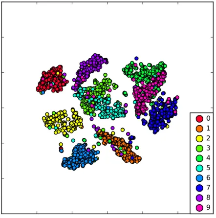
It is necessary to emphasize that the low-dimensional output of t-SNE is based on probabilities, not distances, therefore only relative positions of data points provide informational value of the modelled data. This causes modelled data to be invariant to scale and rotation. Example of t-SNE method used for visualization of handwritten digits can be seen in figure 4.1. In this figure it is possible to see that digits similar in handwriting like 3 and 5 or 7 and 9 are placed relatively close, whereas dissimilar digits like 0 and 9 are placed far apart.
0
1
2
3
4
5
6
7
8
9
Figure 4.1: Demonstration of t-SNE method performance used on MNIST handwritten
digits recognition task1.
1This image was generated using demonstration data distributed with t-SNE implementation inpython
Chapter 5
Implementation of visualisation
system
Chapter 2 – Neural networks and chapter 3 – Automatic Speech Recognition summarize basic theoretical background needed for understanding principles of neural networks and their use in automatic speech recognition. This chapter provides information about system designed for training and visualization of neural networks used for speech recognition. This system can be structurally divided into four parts:
1. Data preparation
2. Neural Network training 3. Activation extraction 4. Activation visualization
5.1
Data preparation
Goal of data preparation is extraction of phonetic features from speech recordings. Kaldi toolkit [12] and its standard scripts were used in this work. The Kaldi toolkit is an
open-source framework for Automatic Speech Recognition providing functions for generating GMM / HMM or DNN / HMM systems, described in section3.1.2. It contains simple command line tools written in C++, which are then called usually from bash, python orperl scripts.
In this work, Kaldi framework was used to extract speech features from AMI dataset IHM sound recordings. These features and AMI dataset labels were used to generate classic GMM / HMM recognition system producing feature alignments dataset for training and testing DNN, as described in section 3.2.
5.2
Neural Network training
Even though the Kaldi framework can be used to train DNNs and first experiments of the term project were based on this toolkit, after recommendations from my supervisor,
Martin Karafiát, CNTK framework was selected for DNN training. The CNTK has better and much simpler neural network design capabilities and it provides simple and efficient way of printing hidden units activations. Moreover it is compatible with Kaldi file format so no file conversions are necessary.
5.2.1 Computational Network Toolkit (CNTK)
TheComputational Network Toolkit (CNTK)[1] is open-source framework for deep learning
developed by Microsoft Research group. In the CTNK, neural networks are represented as computational nodes of directed graph. Leaf nodes of this graph represent input values or network parameters and other nodes represent matrix operations upon their inputs. This representation allows users to easily create and modify various types of neural networks. Another advantage of the CNTK is high performance on multiprocessor machines and high utilization of GPUs. Disadvantage of the CNTK framework is, that it is still in beta phase, so some features are not yet available and bugs are occurring.
5.3
Activation extraction
CNTK scripts similar to the one specified in appendix B.1 was used for activation printing. It prints values of activation functions of hidden units in response to neural network inputs. Activation values from every layer are stored in separate files. These files are formatted as Kaldi binary matrix feature files (sometimes calledark files) with format: utterance_id_key1|BINARY_FLAG|DATATYPE_FLAG|row_count|col_count|data
utterance_id_key2|BINARY_FLAG|DATATYPE_FLAG|row_count|col_count|data utterance_id_key3|BINARY_FLAG|DATATYPE_FLAG|row_count|col_count|data ...
Rows in these records are representing the reaction of hidden layer output to feature frame input indicated by line number in given utterance. Columns in these records are representing individual neuron outputs of specified layer and input. All outputs are floating point numbers with single precision as defined in CNTK configuration scripts.
For reading files containing extracted activations in Kaldi format described above, scripts providing python interface were used. These scripts (kaldi_io.py and htk.py)
were created by Karel Veselý at BUT FIT and are available under the Apache License, Version 2.0 (the “License”). These scripts are reading the activation files one record at
the time thanks to use of python iterators. This comes very handy since activation files tend to be quite big and loading them whole to memory is not possible.
5.4
Activation visualization
For the visualization and analysis of unit activations, special scripts inpython was written.
These scripts are based mainly on the previous work of Khe Chai Sim [16]. The steps of the algorithm for creation of interpretable activity regions and activation visualisation are described in following paragraphs.
5.4.1 Activity vectors
Consider activation value ℎ(𝑖𝑙)(𝑡), which is response of the 𝑖-th neural unit in 𝑙-th layer to
input feature at time 𝑡.
Before all, the activation valuesℎ(𝑖𝑙)(𝑡) extracted from hidden layers must be rescaled to
satisfy conditionℎ(𝑖𝑙)(𝑡) ≥0. This is true for sigmoid and rectified linear units. For LSTM unit, which output is based on hyperbolic tangent function, values must be rescaled using feature scaling normalization:
𝑋′ = 𝑋−𝑋𝑚𝑖𝑛
𝑋𝑚𝑎𝑥−𝑋𝑚𝑖𝑛 (5.1)
Activation values normalised in this way can be used to createactivation vectors which
represent activations of certain unit with respect to given attributes (for example phonemes, speakers or noise types). As proposed by Khe Chai Sim in [16], the activity vector for 𝑆
instances of the observed attribute is defined as:
𝑎𝑖(𝑙)= [𝑎(𝑖𝑙)(1), 𝑎𝑖(𝑙)(2), ..., 𝑎(𝑖𝑙)(𝑆) ] (5.2)
The 𝑠-th element of this vector is then given by: 𝑎(𝑖𝑙)(𝑠) = ∑︀ 𝑡𝛾𝑠(𝑡)ℎ(𝑖𝑙)(𝑡) ∑︀𝑆 𝑠=1 ∑︀ 𝑡𝛾𝑠(𝑡)ℎ(𝑖𝑙)(𝑡) (5.3) Value 𝛾𝑠(𝑡) represents the probability of associating attribute 𝑠 with input feature at
time 𝑡. Usually, number of attribute instances is the number of classes, which the neural
network is supposed to classify. Then 𝛾𝑠(𝑡) is set to 1 if the frame at time 𝑡 corresponds
to correct class, respectively with the data label at time𝑡, otherwise𝛾𝑠(𝑡) is set to 0. The
labels can be represented as probabilities, in which case the value of 𝛾𝑠(𝑡) will represent
confidences of associating attribute 𝑠with given input feature𝑡.
Using normalisation described above, it is evident that 𝑎(𝑖𝑙)(𝑠) ≥ 0 for all 𝑠 and
∑︀
𝑠𝑎
(𝑙)
𝑖 (𝑠) = 1. Based on this, it can be said that the value 𝑎
(𝑙)
𝑖 (𝑠) is weight of hidden
units activation in respect to attribute 𝑠. In other words, value 𝑎(𝑖𝑙)(𝑠) is high when input
acoustic frame belongs to attribute 𝑠and low when it does not.
5.4.2 Normalised entropy
From activation vector 𝑎(𝑖𝑙) can be calculated normalised entropy indicating information
content, respectively sensitivity of given neural network unit 𝑎𝑖 to observed attributes.
Formula for normalised entropy of neural unit𝑎𝑖 is defined as:
𝐸𝑖(𝑙)= − ∑︀𝑆 𝑠=1 𝑎 (𝑙) 𝑖 (𝑠) log𝑎 (𝑙) 𝑖 (𝑠) −∑︀𝑆 𝑠=1 𝑆1 log 1 𝑆 (5.4) Lower entropy value𝐸𝑖(𝑙)corresponds to unit with higher information content and higher
sensitivity to given attribute. In ideal case, unit which has entropy 𝐸𝑖(𝑙) = 0, has perfect
(100 %) sensitivity to one of the attributes and no sensitivity at all to any other attribute. Opposite case is unit 𝑎(𝑖𝑙) which is uniform vector of values 1/𝑆, therefore its entropy is
maximal -𝐸𝑖(𝑙)= 1 and its informational content is none - it is called insensitiveunit. Sim
experiments with entropy based pruning it can be assumed that they have no contribution to the result of classification and they could be pruned from the neural network in order to speed up the system.
5.4.3 Hidden activity space
In order to create interpretable 2D images, 𝑆-dimensional activation vectors need to be
projected to 2-dimensional plane. The t-SNE method, described in section4.2, is used for this projection. This plane is called hidden activity space. Based on the principle of the
t-SNE method, units are positioned with probabilities corresponding to the similarities of their respective activation vectors. That means, units with similar activity vectors are positioned close together and units with different activity vectors are positioned far apart. Units placed in this manner form convex hull. Shape of the convex hull is determined by
most outer units, which are usually units with most entropy, therefore were placed as far
as possible from each other. Since t-SNE place units according with probabilities and not distances, it is not useful to measure distances in hidden activity space, useful information is contained only in relative positions of units. Example of hidden activity space and convex hull without interpretable regions is in figure 5.1.
Figure 5.1: Example of hidden activity space.
It is necessary to note that t-SNE is randomly initialized and also highly data-dependent, because when reducing dimensions, pairwise probabilities are computed for every possible pair of points. In other words significant change in small number of points can entirely change the outcome. Therefore it is not possible to directly compare two visualisations created with different t-SNE projections. Solution to the random initialization is in this work solved by randomly pre-generating more initialization values than it is necessary. These values are then stored in file and loaded every time t-SNE is invoked. This change in t-SNE script does not have severe negative impact on quality
of visualisations, because it is possible to compensate for it with more iterations of the t-SNE algorithm. As for the data dependency problem, even for multiple different data batches to compare, it is possible to perform single t-SNE projection for all data-points as long as dimensions of the activity vectors are identical and they represent identical attributes. This is done simply by horizontally concatenating high-dimensional data points (over all layers of neural network or even over several neural networks), performing the t-SNE projection and afterwards horizontally splitting the low-dimensional vectors. This is possible because t-SNE method preserves order of the data-points. Subsequently can be split portions visualised and compared with each other. Only negative of this approach is that both time and memory complexity of the t-SNE method are 𝑂(𝑛2), so
concatenating large batches quickly becomes very resource-consuming.
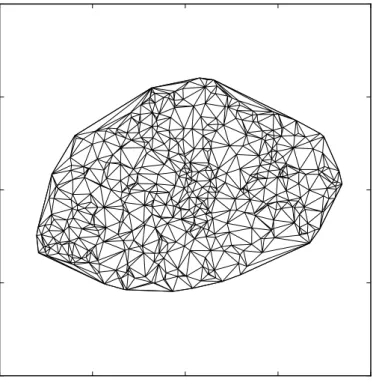
5.4.4 Delaunay triangulation
Algorithm for interpretable regions is dependent on computing Delaunay triangulation on
points of the convex hull resulting from the t-SNE method. Delaunay triangulation was proposed by Boris Delaunay in 1934 [3].
Delaunay triangulation𝐷𝑇(𝑃) is mathematically defined for set of non-linear points𝑃
in a plane. Triangles 𝐷𝑇(𝑃) are constructed in such way that no point from set𝑃 can be
inside of any circle created by circumscribing all triangles 𝐷𝑇(𝑃). When there are more
ways to create triangulation, the way with maximal values of the smallest angles is selected, in order to prevent creation of slim triangles. Example of Delaunay triangulation performed on convex hull points is depicted in figure5.2.
5.4.5 Ranking vectors
Before creating interpretable activity regions, it is necessary to compute ranking vectors.
Ranking vectors are defined as:
𝑟𝑖(𝑙)= [ 𝑟𝑖(𝑙)(1), 𝑟𝑖(𝑙)(2), ..., 𝑟𝑖(𝑙)(𝑆) ] (5.5)
where 𝑟(𝑖𝑙)(𝑠) ∈1, 2, ..., 𝑆 is the rank of attribute 𝑠 computed from activation vector 𝑎(𝑖𝑙)(𝑠) based on formula:
𝑟𝑖(𝑙)(𝑠)< 𝑟(𝑖𝑙)(𝑠′) ⇐⇒ 𝑎𝑖(𝑙)(𝑠)> 𝑎𝑖(𝑙)(𝑠′) ∀ 𝑠, 𝑠′ (5.6)
Practically this means that values of ranking vector represent order of attributes. Attribute for which the 𝑖-th unit activation is highest is ranked first, attribute for which
the unit has the second highest activation is ranked second and so on up to the attribute for which the unit has the lowest activation value which is ranked as𝑆-th.
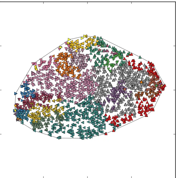
5.4.6 Interpretable activity regions
Interpretable activity regions is the name of the first visualisation method proposed in [16].
Interpretable regions in hidden activity space are created according to following steps: 1. Find a seed unit 𝑂𝑠 for each observed attribute 𝑠. The seed unit has the largest
average activity value computed from itself and its immediate neighbours in Delaunay triangulation.
2. Use the seed units to initialise their respective regions: 𝜌𝑠={𝑂𝑠 };
3. Set the ranking threshold to 𝑟*= 1;
4. For each attribute𝑠, recursively add all units,
which satisfy condition 𝑟(𝑖𝑙)(𝑠)≤ 𝑟* and are connected by Delaunay triangulation to
units in region.
5. Increment the threshold: 𝑟*=𝑟*+ 1;
6. If𝑟* ≤𝑆, go to step4;
First seed units for each observed attribute are found. Subsequently seed units are used to initialize activity regions, which are incrementally expanding by including neighbouring units with higher or equal activation values (which are represented by lower or equal rank values) for current attribute. Adding of units continues until all units belong to some attribute.
For this work slight modification of the above algorithm was used. Instead of recursively adding neighbouring units, units were added iteratively. Iterative adding resulted in slightly more fair region creation since there were more cycles of the algorithm and therefore assigning of the units with high entropy (and low information value) is less dependant on the order of attributes in algorithm and more dependant on the activation values.
Example visualisation of neural units in hidden activity space using modified algorithm is depicted in figure5.3.
5.4.7 Interpretable regions in 3D
Algorithm described in previous sections can be easily generalized for more than 2 resulting dimensions, because t-SNE method is capable of transforming its high
dimensional input data to any dimension lower than the input dimension. The Delaunay triangulation can also be generalized to higher dimensionality — for example in three-dimensional space, tetrahedrons are created instead of triangles and are inscribed in spheres instead of circles. All other parts of the algorithm are invariant to change of output dimensionality. Example visualisation of neural units in three-dimensional hidden activity space is depicted in figure 5.4. Although creating three (and theoretically even more) dimensional regions is possible and should retain more information than 2D visualisation, interpretation of such visualisations is difficult, therefore it is not used in experiments of this work, but it is worth to note such possibility exists.
Figure 5.4: Example of interpretable regions in 3D space. (Only three groups of attributes are shown for clarity.)
5.4.8 Activity visualisation
Activity visualisation is alternative visualisation method proposed in [16]. Creating
visualisations of hidden units activities is also dependent on producing hidden activity space by t-SNE method as described in section 5.4.3. Similarly to creation
of interpretable activity regions, Delaunay triangulation is performed over all units creating triangular mesh. Every vertex of this triangular mesh is representing hidden unit
in activity space. To these units — vertices are assigned activation values of particular observed attribute instance from activity vector (described in section 5.4.1) corresponding to the individual unit. Subsequently, these activation values are converted to colours using suitable colour map. Finally, triangles produced by Delaunay triangulation are filled with colour gradient based on colours, respectively activations of their respective vertices.
Example of activity visualisation of three different attribute instances (phonemes /sil/, /AH/ and /S/) visualised for every layer of selected neural network is in figure 5.5.
For conversion of unit activity to colour in this example, jet colour map was selected.
Using jet colour map, red colour corresponds to high activation values and blue colour indicates low activation values of hidden units. This method makes possible to observe changes in activations corresponding to selected attribute instance over all layers of neural network. It would be even possible to observe these changes over time, although such experiment would require to snapshot activation values in every discrete time step, which would require tremendous amount of computational resources.
/𝑠𝑖𝑙/
/𝑆/
/𝐴𝐻/
𝐿𝑎𝑦𝑒𝑟 1 𝐿𝑎𝑦𝑒𝑟 2 𝐿𝑎𝑦𝑒𝑟 3 𝐿𝑎𝑦𝑒𝑟 4 𝐿𝑎𝑦𝑒𝑟 5 𝐿𝑎𝑦𝑒𝑟 6
Figure 5.5: Example of activation visualisations ofphonemes /sil/, /AH/ and /S/ over all
Chapter 6
Experiments
Since this work deals with visualisations of neural networks used in ASR, for experiments in this work was selected the most basic task of this field — the phoneme recognition.
Following sections discus choice of the dataset, modifications in approach of visualisation, neural network architectures and interpretations of resulting visualisations.
6.1
Dataset description
The AMI Corpus dataset was selected for experiments with retrieving activations from
NN. Main reason for this selection was, that this dataset is well established in community of automatic speech recognition, and there are prepared examples for its use in most of the ASR frameworks like Kaldi or CNTK.
AMI (Augmented Multi-party Interaction) corpus is multi-modal data set consisting
of 100 hours of conference room meeting recordings, intended for developing meeting browsing technology. This work will concern only with the audio part of the dataset. The audio data are divided into three parts based on microphone devices used for recording:
∙ Independent headset microphone (IHM) ∙ Multiple distant microphone(MDM) ∙ Single distant microphone(SDM)
Multiple distant microphone part of the corpus was recorded with microphone array put on the table. Single distant microphone part was generated as output of one of the microphones in array. Unfortunately, these parts are considerably suffering from microphone and environment noise, which presents itself also in speech recognition results in comparison to IHM data part. For this reason, only the IHM data part was used in experiments for neuron activations extraction.
The IHM data part contains 27 822 979 frames in 108 221 utterances. Features used in neural network training were computed by standard AMI recipe for Kaldi. Type of the features is MFCC (see section 3.1.1) with Constrained Maximum Likelihood Linear Regression for speaker adaptation.
6.2
Compensating dataset statistical characteristics
In first experiments with interpretable region visualisations of neural networks came up problem with large regions of one or more frequent attributes (e.g /sil/, /S/, /AH/ phones in phoneme recognition), which covered more than 90% of all units in every layer and every
architecture type. This is caused by the statistical imbalance of input data. Large portion (almost 25%) frames of the dataset is actually silence and the rest of the frames is more or less evenly distributed amongst other 42 phonemes. This way the average portion of frames for phone other than silence is under 1.8% of dataset frames. When majority of the units
have very high rank for silence, they are “swallowed” by it in the recursive part of the algorithm. This problem occurred most evidently in visualisations depicting individual layers transformed by the t-SNE method given only data of the single respective individual layer.
Because visualisations taken over almost entirely by the silence or another very common phones like /S/ or /AH/ have almost none informational value, two modifications of the
visualisation algorithm were suggested. These modifications are described in following subsections.
6.2.1 Attribute occurrence normalisation
First option is to weight individual phonemes by number of occurrences of given phoneme in the dataset. This effectively changes the equation (5.3) to:
𝑎(𝑖𝑙)(𝑠) = ∑︀ 𝑡𝛾𝑠(𝑡)ℎ (𝑙) 𝑖 (𝑡)w(s) ∑︀𝑆 𝑠=1 ∑︀ 𝑡𝛾𝑠(𝑡)ℎ(𝑖𝑙)(𝑡) (6.1) where 𝑤(𝑠) is the relative number of occurrences of attribute 𝑠 in the dataset. This
results in more evenly distributed values in activation vector, which subsequently results in higher entropy for neurons and more evenly distributed ranks. This manifests itself in the higher number of smaller attribute regions in resulting visualisations. Although this method artificially minimizes regions with large occurrence rate it provides the detailed view on the rare units.
6.2.2 Silence trimming
This solution is particular to visualisation of phoneme recognizing neural networks on dataset with very large ratio of silence in data. Since main purpose of silence is only to divide words, it is possible to discard large portion of it by restricting the sequences of silence in the dataset to maximal value of 15 consecutive frames. This modification of the dataset shows benefit in visualisations, because more attributes can take up the units usurped by the silence region.
Sadly, this approach cannot be used when dealing with large counts of phones other than silence and also it cannot be used for other other types of attributes, but it can be generalized to selecting statistically uniform subset of the dataset and use it for the neural network training. Of course in this way characteristics of the original dataset are lost, but such approach could be useful in comparison of different visualisation methods. Visualisations using the uniform subset should be similar to the ones using attribute occurrence normalisation described in section6.2.2.
![Figure 3.1: Automatic speech recognition system [18].](https://thumb-us.123doks.com/thumbv2/123dok_us/11087410.2995766/17.892.153.790.635.889/figure-automatic-speech-recognition-system.webp)