Bayesian Nonparametric Methods with Applications in Longitudinal, Heterogeneous and Spatiotemporal Data

(1)

(2)

Bayesian Nonparametric Methods with

Applications in Longitudinal, Heterogeneous and

Spatiotemporal Data

A dissertation submitted to the Graduate School

of the University of Cincinnati in partial fulfillment of the requirements for the degree of

Doctor of Philosophy

in the Department of Mathematical Sciences of the College of Arts and Sciences

by Li Duan April 2015

Doctoral Committee:

Xia Wang, Ph.D., Chair Siva Sivaganesan, Ph.D. Seongho Song, Ph.D. Emily Kang, Ph.D.

(3)

ABSTRACT

Bayesian Nonparametric Methods with Applications in Longitudinal, Heterogeneous and Spatiotemporal Data

by Li Duan

Nonparametric methods provide flexible accommodation to the different structures in the data without imposing strong assumptions. Bayesian consideration of nonpara-metric models, such as Gaussian process, Dirichlet process and decision tree enables straightforward computation and automatic regularization. In this dissertation, we developed three novel nonparametric methods for handling different types of data. For the longitudinal and time-to-event data, we utilized the multiple subject compo-sition and repeated measurement, and designed a hierarchical Gaussian process that enables extrapolation for personalized forecast. For the regression of heterogeneous data, we combined the clustering properties of the Dirichlet process and the nonlin-ear incorporation of predictors in decision tree, and developed an efficient method for handling heterogeneity and ensemble estimation. For the spatiotemporal data, we first designed a performant algorithm for stationary Gaussian process, and then extended it to allow non-stationarity and non-Gaussianness of the complex data. We demonstrate the advantages of the Bayesian modeling in latent variable sampling, missing data handling, algorithm acceleration, accurate prediction and probabilistic interpretation.

(4)

(5)

ACKNOWLEDGMENTS

I have been most fortunate to work with two of the most talented statisticians in the world, whom I owe my greatest gratitude to. My advisor, Professor Rhonda Szczesniak from Cincinnati Children’s Hospital, gave me tremendous support and freedom in exploring my academic interest. She spent countless hours in discussing project progress, revising my publication drafts, finding grants to support me, en-couraging me to compete for awards and supporting me to national conferences. She taught me the strategy to tackle the problems with analytical plans, the wisdom to answer the question with statistical tools and the language to make impact in the real world. My dissertation advisor, Professor Xia Wang from University of Cincin-nati, guided me into the marvelous world of Bayesian statistics. She taught me the importance of data-driven modeling and the gracefulness of parsimonious methods. Without their guidance and help, the completion of this dissertation would not be possible.

I would like to thank my committee faculty members, Professors Siva Sivaganesan, Seongho Song and Emily Kang, for the invaluable lectures in the past few years and useful advices during forming this dissertation. I would also like to thank our collaborators from Cincinnati Children’s Hospital, Professors John Clancy and Raouf Amin for providing support and data for these analyses.

Personally, I want to thank my dearest wife, my supportive parents and my in-spiring uncle and aunt. It is them that keep me going in my life.

(6)

LIST OF FIGURES

Figure

1.1 Illustration of a decision tree . . . 5

2.1 Forecasting using HGP model results in better mean estimates and

regulated prediction errors, compared with using only one Gaussian

process . . . 14

2.2 Estimation of the latent processes using JHGP model in simulation

studies. The true unknown processes are shown in blue, and the estimated values and the 95% pointwise credible intervals are shown

in red. . . 20

2.3 Different types of covariance functions in the individual process leads

to different extrapolation curves (solid lines on the right). . . 21

2.4 Sensitivity-specificity analyses in simulation studies. From up-left to

the diagonal, ROC curves (AUC) of model fitted with: JHGP (0.828),

extended HGP(0.782), logistic regression (0.626). . . 23

2.5 Forecasting performance in simulation studies. Comparison plots of

the predicted vs the true values. . . 24

2.6 Fitted values of FEV1% and PEx hazard with JHGP model on CF

data . . . 27

2.7 Forecasting performance in FEV1% of CF data. Comparison plots of

the predicted vs the true values. . . 27

2.8 Forecasting in FEV1% using two hierarchies of Gaussian process. The

population smoothed line (adjusted with individual intercept) are shown in red; and individualized AR(1) prediction is shown in blue.

The 95% credible intervals are also included. . . 28

2.9 ROC curves of fitting using CF data: JHGP (blue) shows higher AUC

at 0.735, followed by extended HGP (red 0.683) and simple logistic

regression (black 0.605). . . 28

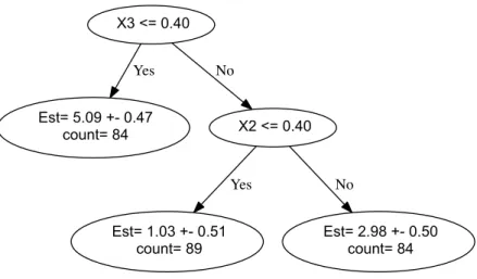
3.1 Simulation Study I shows one cluster is found and the partitioning

scheme is correctly uncovered . . . 40

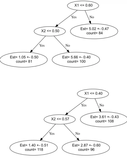
3.2 Simulation Study II shows two clusters are found and parameters are

(10)

3.3 Simulation Study III has data from different partitioning schemes mixed together. The means are labeled in the center of each region.

The shared region in the upper left has mixed means. . . 43

3.4 Simulation Study III shows two clusters correctly identified . . . 44

3.5 Result of breast cancer test . . . 46

3.6 Results of FEV1% fitting and prediction. . . 49

4.1 Illustration of edge effect using a 50×50 matrix with squared expo-nential covariance and range ρ = 3. If the data of interest has size N = 50 and no augmentation is used, then the edge effect on the corners would impact the likelihood. However, if the data of interest has size N ≤40 andNaug = 50−N, then the edge effect would have no impact on the likelihood of the N data. . . 64

4.2 Simulation of a nonstationary Gaussian process: Z(s) = sin(exp(s· π/500/0.7)) +s, s iid ∼ N(0,0.01) for s= 1,2, ...500 . . . 71

4.3 Simulation of a nonstationary and non-Gaussian process: a mixture of two stationary Gaussian processes with two different frequencies and mixture weights ωl=1(s) = |sin(s·2π/500)| . . . 72

4.4 The four stationary components estimated by the time-space inter-active model _M(N S) using generalized functional Gaussian process (GFGP) model. The estimated mean process µ_k and weight pro-cess ωk in each component are shown. Each mean processes µk has distinct smoothness and exhibits changes over the time; while each weight process ωk shows geographical clustering and appears unchanged over time. . . 76

4.5 Comparison of the original temperatures in the dataset and the pre-dicted ones generated by the space-time interactive model _M(N S). . 78

4.6 Plot of the covariance as the space distance x2 _{or the time distance} |t| increases. . . 79

A.1 Variable importance calculated by Random Forests with 50 trees, using cystic fibrosis data. . . 92

A.2 Cluster 1 found by the BET model applied on the cystic fibrosis data 93 A.3 Cluster 2 found by the BET model applied on the cystic fibrosis data 94 A.4 The 3 stationary components estimated by the GFGP in _M(A) and M(S). Due to the limited flexibility in M(A), its weight process cannot fit the data as well as the other two models. . . 95

(11)

CHAPTER I

Introduction to Bayesian Nonparametric Methods

It often relies on strong assumptions to assign parametric models in the data anal-ysis. As an extreme example, a simple linear regression implies at least four require-ment for the data: linearity, independence, normal distribution and homogeneity. As we have commonly witnessed in real life, these assumptions are often violated. Data may exhibit nonlinear progress over time, correlation over space and time, more than one patterns (heterogeneity), etc. For such cases, sometimes parametric methods might still work and even show robustness despite of the misspecification; however, these analytics can be dramatically improved if we obtain a better understanding of the data and accommodate their features.

Nonparametric methods provide attractive solutions to these challenging prob-lems. By only enforcing properties such as smoothness on the nonparametric esti-mates, we can relax the assumptions about the data. Instead of prescribing rigid distribution, we allow the model to be flexible and adaptive to the different charac-teristics in the data. To clarify, most of nonparametric models do have parameters. The difference is that instead of directly representing a parametric form (such as in-tercept and slope), these parameters are related to more implicit properties of the data, such as correlation pattern, latent class distribution, etc. Similar to the ones in parametric models, the values of the parameters will also influence the

(12)

goodness-of-fit, therefore require proper procedure in their estimation. This naturally leads to another question: how do we balance model flexibility and overfitting (i.e. mistaking random noise as systematic patterns)?

This question has an elegant answer in Bayesian framework: if we adopt the nonparametric models into the prior distribution, its parameters will be automati-cally tuned by the data, and the posterior distribution become the nonparametric estimates. From a regularization standpoint, the prior distribution shrinks the mag-nitude of the posterior estimates and penalize aggressive fitting.

In this dissertation, we utilize three families of Bayesian nonparametric methods

1 _{and the combination of them, in order to address the special structure of the data.}

In this section, we briefly review the basic properties of these methods.

1.1 Gaussian Process

Gaussian process is commonly used to model the nonlinear function for the con-tinuous data. When the data are assumed to have a specific covariance function, it is equivalent to adding a regularization based on reproducing kernel Hilbert space (Lawrence and Jordan, 2004). Moreover, the finite-dimensional distribution of a Gaussian process has the measure of a multivariate Gaussian distribution.

We assume that the continuous data Y scattered over a set of location/time s

are a vector of noisy realization from an underlying process, to which we assign a Gaussian process prior:

Y =f(s) +

f(s)∼GP(µ,Σ(s))

(1.1)

where Σ is restricted to a specific functional forms, such as φ2exp(−||s1 −s2||2/2ρ)

1_{To avoid confusion, we use the term “Bayesian nonparametrics” as a broader concept as any}

nonparametric method with Bayesian treatment, in contrary to the one referring Dirichlet process alone in some other literature.

(13)

for the correlation between data points ats1 ands2. For simplicity of illustration, we

assume iid∼N(0, σ2_{)). The posterior distribution of}_f₍_s_{) then follows a multivariate}

Gaussian distribution:

f(s)|Y ∼N(µ∗,Σ∗)

µ∗ =µ+Σ(Σ+σ2I)−1(Y −µ)

Σ∗ =Σ−Σ(Σ+σ2I)−1Σ

(1.2)

Although the derivation of the distribution seems trivial, one important feature is

that the posterior meansµ∗will inherit the special properties of the prior distribution.

Examples of these properties include differentiability, frequency, stationarity, etc.

From a signal processing standpoint, applying functional form to Σ is equivalent to

adding a filter (Σ(Σ+σ2I)−1) and only let specific range of frequencies to pass (more

will be illustrated in Chapter IV).

A different focus of using Gaussian process prior is to understand the correlation structure of the data. As the correlation matrix is an integral part of the multivariate Gaussian distribution, using a functional form with a few parameters to represent a large matrix can be quite beneficial. This is one of the reasons Gaussian process

prior has wide range of applications in spatial statistics (Cressie, 1988). Utilizing the

equations in (1.2), the form of µ∗ is also known as Kriging estimator and shown to

be the best linear unbiased predictor (BLUP).

The use of Gaussian process prior will be illustrated in Chapter II as a function estimator, and as in Chapter IV as a covariance structure model. In Chapter IV , the limitations of Gaussian process will be thoroughly discussed and new efficient solutions will be presented.

(14)

1.2 Dirichlet Process

Dirichlet process provides a probabilistic framework used to model mixture

dis-tribution (Neal, 2000). For this reason, it can be particularly useful in modeling

heterogeneous data, which contain more than one distributional patterns.

The notation of a Dirichlet process Y∼DP(α, G) can be interpreted as the

fol-lowing generative model, for the ith data point:

p∼Dir∞(α, α, ...) Ci|p iid ∼M N∞(p) Yi|Ci indep ∼ GCi (1.3)

whereDir∞ andM N∞ represent infinite dimension Dirichlet and multinomial

distri-bution, respectively. The symbol C is the latent random variable that carries class

assignment, and G is called the base distribution and can take form of any

distri-bution with finite measure. One simple example of Dirichlet process is an infinite mixture of Gaussian distribution with the weights following a Dirichlet distribution. Similar to the Gaussian process, one of the most important features of Dirichlet process lies in its posterior distribution:

p|Y, C ∼Dir∞(α+ X i 1(Ci = 1), α+ X i 1(Ci = 2), ...) Ci|Yi,p∼M N∞(p1[G1(Yi)], p2[G2(Yi)], ...) (1.4)

where Y are the vector of all the data, and P

i1(Ci =k) denotes the count of data

points that are assigned to kth class, [Gk(Yi)] is the probability measure of Yi in kth

base distribution. Due to the finite number of data points, the probability distribution

in p|Y, C becomes uneven, as the class with more data assignment becomes further

more likely to get chosen. This leads to self-reinforcing clustering of data that only a small finite number of classes are found when the algorithm converges. In the area of

(15)

clustering methods, Dirichlet process belongs to fuzzy clustering (Bezdek, 1981) since the class assignment has randomness as opposed to being completely determined.

The use of Dirichlet process prior will be illustrated in Chapter III and IV. Uti-lizing its properties, we obtain models with better parsimony and accommodation for non-Gaussian and non-stationary data.

1.3 Bayesian Decision Tree

The previous two methods provide flexible accommodation to the data, mainly via relaxed assumptions about the response variable. The third class of model, decision tree method, addresses the nonlinear relationship between response and predictor variables. Considering the nonlinearity in several predictors can be quite costly in linear regression. This is where decision tree method can help since its recursive splitting partitioning automatically incorporates nonlinearity of the predictors.

X2 <= 4.00 X6 <= 2.00 Yes Est= 0.99 count= 175 No X3 <= 1.00 Yes X1 <= 5.00 No Est= 0.00 count= 326 Yes X8 <= 2.00 No Est= 0.01 count= 75 Yes Est= 0.34 count= 13 No X2 <= 1.00 Yes Est= 0.96 count= 41 No Est= 0.02 count= 21 Yes X6 <= 5.00 No Est= 0.38 count= 15 Yes Est= 0.98 count= 17 No

(16)

Decision tree, also known as Classification and Regression Tree (CART) (Breiman et al., 1984) can be viewed as a predictor-based partitioning functionRi =T(Xi) that

transform a vector of information in ith subject into a region Ri, in which region an

estimator is provided for the data within. The partitioner, or the “tree”, is generated by a series of binary splitting with respect to the predictor variables; at each split, a predictor and a corresponding threshold value is used to sort data points. The

building unit is called “node”. If theidata has predictor smaller than or equal to the

threshold, it is sorted to the left descendant; otherwise to the right. This process is repeated until the end of line is reached. For example, in Figure 1.1, one data points

withX1 = 3, X2 = 3, X6 = 4 will be sorted to the first partition on the last row, with

an systematic estimate of 0.38 for its response variable Yi. As the sorting process

involve multiple times of splitting in X2, X6, it approximates the nonlinearity as a

step function with multiple breaks .

It used to be a challenging issue in the estimation of the decision tree. Due to the cost function is not convex, the suboptimal solution relies on local maximization at every split. To prevent overfitting, empirical constraints on depth of the tree and pruning procedures are often needed.

Bayesian treatment has greatly improved the estimation and overfitting issues.

As proposed by Chipman et al. (1998), if we assign a likelihood function G to each

partition and treat the overall tree structure as the prior distribution, then we can obtain tree estimation by sampling in its posterior distribution:

Yi ∼GRi Ri =T(Xi) [T] =Y k [sk] (1.5)

where [T] is the prior distribution for the tree, which is the product of the probability

(17)

increases. This automates the control of tree depth and encourages parsimonious model.

Details of Bayesian decision tree will be discussed in Chapter III, including its drawbacks and common remedies. An improved ensemble approach is proposed as part of this dissertation research.

1.4 Overview

The following chapters document three independent topics of research work that are motivated by different types of data. Chapter II extends Gaussian process into joint modeling of longitudinal and time-to-event data. Chapter III uses the com-bination of Dirichlet process and Bayesian decision tree to create a new ensemble method that accommodate the need for nonlinear modeling of heterogeneous data. Chapter IV develops an efficient algorithm for the Gaussian process approach, which is utilized to extend to non-stationary modeling of spatiotemporal data.

(18)

CHAPTER II

Hierarchical Gaussian Process in the Joint

Modeling of Longitudinal and Time-to-Event Data

In this chapter, a novel extrapolation method is proposed for longitudinal forecast-ing. A hierarchical Gaussian process model is used to combine nonlinear population change and individual memory of the past to make prediction. The prediction error is minimized through the hierarchical design. The method is further extended to joint modeling of continuous measurements and survival events. The baseline hazard, covariate and joint effects are conveniently modeled in this hierarchical structure. The estimation and inference are implemented in fully Bayesian framework using the objective and shrinkage priors. In simulation studies, this model shows robustness in latent estimation, correlation detection and high accuracy in forecasting. The model is illustrated with medical monitoring data from cystic fibrosis (CF) patients. Esti-mation and forecasts are obtained in the measurement of lung function and records of acute respiratory events.

2.1 Introduction

Forecasting for stochastic processes is commonly needed in geology, finance and clinical research; however, it is widely known that extrapolation is difficult and risky.

(19)

Since the knowledge is limited to only the observed domain, without theoretical evi-dence, researchers tend to use simple functions for extrapolation. Except for its con-servativeness, this practice is often unrealistic and overlooks many intrinsic properties, such as nonlinearity and stochastic fluctuations. This problem has been ameliorated by development in two fields of studies: time series and longitudinal data analysis. In the former, the variation in the past helps prediction in the future by the recursive relations. In the latter, the trend shared in batch data provides a reasonable guess for a given individual. Therefore, it is desirable to find a method that unifies these two fields.

In estimating the time-varying process behind the noise, nonparametric approaches

such as penalized B-splines (Eilers and Marx, 1996) have been quite successful.

How-ever, one of the limitations is the subjective allocation of knots. For individual traces with only a few recorded points, it is still difficult to avoid over-fitting. Although

methods like Bayesian Adaptive Regression Splines (BARS) (DiMatteo, Genovese,

and Kass, 2001) have been proposed to address such issue, it is not feasible to use it for extrapolation.

An alternative approach is Gaussian process regression (GPR) (Rasmussen and

Williams, 2006). By using a small number of (quite often as low as 1) parameters and a smooth covariance function, GPR avoids the use of knots and keeps the di-mension fixed. This enables a fast estimation without sacrifices in robustness. In

Eqn 1.1, assume Y is a stochastic realization of time dependent function f(t), with

∼N(0, σ_y2I). Iff(t) is a Gaussian process andΣis formed by a covariance function

that is differentiable with respect to time increments, then the posterior mean will also be a differentiable (smooth) function.

Major progress has been made in its predicting ability. For example, the Kriging estimator has been shown to be the best linear unbiased predictor (BLUP) and has

(20)

denote the time vector of observed data, s to denote the vector of prediction time

and K(s,t) to denote the their covariance:

f(s)|Y(t)∼N(µ∗,Σ∗)

µ∗ =µ(s) +K(s,t)(Σ(t)+σ_y2I)−1(Y(t)−µ(t))

Σ∗ =Σ(s)−K(s,t)(Σ(t) +σ_y2I)−1K0(s,t)

(2.1)

The magnitude of K(s,t) is usually reversely dependent on the distance measure

||si −tj||. In interpolation, these distances remain moderate since s is inside the

domain oft; whereas in extrapolation, all|si−tj|increase monotonically. As a result,

the prediction mean monotonically reduces to µ(s) and prediction variance increases

toΣ(s). Therefore, slowing down the reduction ofK(s,t) and improving the estimate

of µ(s) are essential to achieve reasonable forecasting results. The Gaussian process

functional regression (GPFR) model (Shi, Wang, Murray-Smith, and Titterington,

2007) was proposed to solve this problem. Similar to longitudinal data, the data described by Shi and colleagues are collected in batches. In the first step, B-splines

are used to estimate the batch mean att and s; in the second step, this mean is used

as µ(t) and µ(s) for individual extrapolation. This approach greatly improves the

forecasting ability of Gaussian process.

On the other hand, if the longitudinal data are collected at the same time as a related survival event, a joint model is commonly adopted for improved estimation and inference. Longstanding motivation for methods to link longitudinal and

time-to-event data originated from human immunodeficiency virus (HIV)(Song, Davidian,

and Tsiatis, 2002). Most recent developments of joint longitudinal-survival models have been accompanied by online calculators for the purposes of real-time

individ-ual prediction of prostate cancer recurrence (Taylor, Park, Ankerst, Proust-Lima,

Williams, Kestin, Bae, Pickles, and Sandler, 2013). Nevertheless, some challenges remain in the field of joint modeling: the estimation is difficult in the baseline hazard

(21)

and full likelihood; the forecasting is unstable, especially in recurrent survival event modeling; the association between two responses lacks a realistic interpretation. The

survival function specified in the Cox relative risk model (Cox, 1972) takes the form

of Eqn 2.2. S(T ≥t2|T > t1) =exp{− t2 Z t1 λ0(u)exp{Xβ+f(u)}du} (2.2)

The use of t1 is to accommodate the possibility of a recurrent event. In the case

of nonrecurring events, we simply set t1 = 0. Since the data are collected at discrete

time points, approximation is usually needed to evaluate the integral. However, if one

needs to forecast multiple time points corresponding to recurring events,t1 is random

and Eqn 2.2 becomes intractable. To tackle these problems, we adopt the discrete

Cox relative risk model provided in the same article (Cox, 1972). The estimation and

prediction now have a tractable solution in closed form. Details are described later in section 2.2.

The major novelty in our approach is that we use two hierarchical Gaussian pro-cesses for both longitudinal and survival submodels. In the longitudinal part, the first hierarchy enables the sharing of the trajectory trend among subjects; and the second captures the individual deviations through a time-series covariance function. In the survival part, the first Gaussian process acts as a smoother for the baseline; the second Gaussian process serves as a time-varying frailty term. Using the of shared

parameter framework (Vonesh, Greene, and Schluchter, 2006), we set up the

associa-tion between the two responses through a time-varying covariance. This hierarchical structure enables a reliable extrapolation by combining a nonlinear population trend, individual autocorrelation and joint effect. The model is straightforward and the estimation procedure is completely likelihood-driven and single-staged. The compu-tation is demonstrated in a fully Bayesian framework and Expeccompu-tation-Maximization

(22)

algorithm.

The remainder of the chapter is organized as follows. In Section 2, we present details for the proposed hierarchical Gaussian process (HGP) model, its extension as a survival model and the joint hierarchical Gaussian process (JHGP) model. In Section 3, we present the simulation studies and assess forecasting performance. In Section 4, we apply the JHGP model to clinical data from patients with cystic fibrosis. Concluding remarks and discussion are presented in Section 5.

2.2 Methods

2.2.1 Hierarchical Gaussian Process Model 2.2.1.1 Model Structure

The records ofYij’s are assumed to be from a continuous stochastic processYi(t)

of subject i at the jth time interval (i = 1, ..., n and j = 1, ..., ni). For simplicity of

notation, we disregard other covariate effects for now and assume:

Yi(t) =fi(t) +where ∼N(0,Iσy2) fi(t)|µy indep. ∼ GP[µ_y +γi1,Vψσ2ψi] for i= 1, ..., n µ_y ∼GP[0,Vµyσ 2 µy] (2.3)

It is worth noting that there are multiple independent copies offi(t) but only one

copy of µ_y. In other words, µ_y is the shared mean process for all subjects. The time

span of µ_y is equal to the full span of the longitudinal data, where one of the fi(t)

functions is limited to the subject’s first and last observation (or censoring) time.

We addγi to accommodate individual differences at the beginning of each trajectory.

Each individual has a different scale parameter σ2_ψ, but shares the same correlation

matrix Vψ.

(23)

gen-erateVµy. One example of such a function is the squared exponential{exp(−

(∆t)2

2λ2 )}i,j.

This guarantees that µ_y is a smooth function in time. The differentiability replaces

the role of knots in spline-based approaches, thereby avoiding the dimension change problem. On the other hand, we choose a non-differentiable time-series function to

generate Vψ. For example, we use an AR(1) covariance {ρ|i−j|}i,j (−1 < ρ < 0) to

forcefi(t) to have a trajectory that resembles random walk.

2.2.1.2 Predictive Distribution

Forecasts fi(s) at time vector s can then be obtained by conditioning on µy,

Vψσψ2i and Yi(t). f_i(s)|µ_y,Vψ,Yi(t)∼N(µ∗,Σ∗) µ∗ =µ_y(s) +γi1s+K(s,t)(Vψσ2ψi+σ 2 yI) −1₍_Y₍_t₎₋_µ y(t)−γi1t), Σ∗ =Σ(s)−K(s,t)(Vψσ2ψi +σ 2 yI) −1_K0 (s,t)) (2.4)

which is similar to Eqn 2.1. The main difference in Eqn 2.4 is that µ_y(s) and µ_y(t)

are now subsets of µ_y, which is a Gaussian process instead of a simple function.

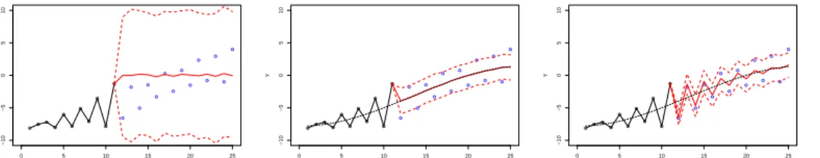
The benefits of having two Gaussian processes for prediction are illustrated in

Figure 2.1. The test samples are first generated in batch (n= 50), then we randomly

select one subject and remove the corresponding second half of the observed points (shown in blue). We first fit each subject with an individual Gaussian process with the AR(1) covariance (Figure 2.1(a)). Although the fitted (black) line shows that the model has adequate flexibility, it cannot perform well in extrapolation: the red line rapidly reverts to the constant mean. This behavior is due to the small

autocorre-lation (ρ close to 0), caused by the heterogeneity of the observation. We next fit all

subjects with a common Gaussian processµwith the squared exponential covariance,

(24)

(Fig-ure 2.1(b)). The prediction benefits from the similarity of trajectories among all the

subjects. Since Y −µ_y is more homogeneous than Y, we use the second

individ-ual Gaussian process (AR(1)) conditional on the estimate of µ (Figure 2.1(c)). The

magnitude of autocorrelation becomes larger (ρ=−0.8) and the decrease of K(s,t)

becomes slower. As a result, both the point estimates and credible intervals of the forecast greatly improve and become personalized.

● ●● ● ● ● ● ● ● ● ● 0 5 10 15 20 25 −10 −5 0 5 10 t Y ● ● ● ● ● ● ● ● ● ● ● ● ● ●

(a) Prediction using the au-tocorrelation of one Gaus-sian process ● ●● ● ● ● ● ● ● ● ● 0 5 10 15 20 25 −10 −5 0 5 10 t Y ● ● ● ● ● ● ● ● ● ● ● ● ● ●

(b) Prediction using the

es-timated µ from the other

subjects ● ●● ● ● ● ● ● ● ● ● 0 5 10 15 20 25 −10 −5 0 5 10 t Y ● ● ● ● ● ● ● ● ● ● ● ● ● ● (c) Extrapolation based on

µand the autocorrelation

Figure 2.1: Forecasting using HGP model results in better mean estimates and reg-ulated prediction errors, compared with using only one Gaussian process

2.2.2 Extension to the Survival Model 2.2.2.1 Model Structure

The Cox relative risk model (Cox, 1972) has been widely used in survival analysis.

We show the HGP can be adopted into the Cox model, thereby enabling forecasting with survival data.

As previously mentioned in Section 1, the discrete Cox model avoids the numerical integration, provides a closed-form solution to the baseline estimates and also the flexibility to incorporate recurrent events. The data set of discrete survival event

is formed in the following procedures: for every event or censoring time t, assign it

into discrete slot k; create the corresponding binary variableRk that takes value 1 if

(25)

period; then fill all the periods between the 0 and k with Rj = 0; in the case of a

recurrent event, fill all the periods between two consecutive events with Rj = 0. Let

λi(k) = P(Rk = 1|R{j:l<j<k} = 0), where l is either the start time or the time of the

last event if it is recurrent. The resulting λi(k) is referred to as the discrete hazard

function of individuali at timek. The full likelihood of a survival event or censoring

can be expressed as P(Rk = 1, R{j:l<j<k} = 0) =λi(k) k−1 Y j=l+1 {1−λi(j)} P(Rk = 0, R{j:l<j<k} = 0) = (1−λi(k)) k−1 Y j=l+1 {1−λi(j)} (2.5)

If we let λ0(k) denote the value of the baseline hazard at time k, then the discrete

Cox relative risk model (Cox, 1972) can be defined as:

λi(k)

1−λi(k)

= λ0(k)

1−λ0(k)

exp{Xiβ+gi(k)} (2.6)

where Xiβ represents the covariate effects and gi(k) is the time-dependent frailty.

By logarithm transformation, we have the equation:

logit(λi(k)) =logit(λ0(k)) +Xiβ+gi(k)

For ease of notation, we ommit Xiβ in the following equation. Since the baseline

hazardλ0 is commonly assumed to be continuous and smooth, thelogit link function

is also a continuous and bijective function; therefore, the logit(λ0) should also be a

smooth function. Analogous to the two hierarchies in HGP, the baseline is a common

smooth process shared by all subjects, the frailty gi is a subject-specific deviation. It

is natural to use HGP to model these two processes.

For simplicity of notation, we use Hi = logit(λi) and µH = logit(λ0). The

(26)

λi = exp(Hi) 1 +exp(Hi) Hi|µh indep ∼ GP(µ_h+ηi1,Vhσ2hi) µ_h∼GP(0,Vµhσ 2 µh) (2.7)

where ηi provides an intercept shift relative to the baseline hazard, in order to

ac-commodate diversity at the starting level. Note that the predictive distribution in Eqn 2.7 is similar to Eqn 2.4.

2.2.3 Joint Hierarchical Gaussian Process Model 2.2.3.1 Model Structure

When continuous measurements and survival events are modeled jointly, the joint

likelihood is factorized according to shared random parameter model (Vonesh, Greene,

and Schluchter, 2006):

P(R,Y) = Z

P(R|ψ)P(Y|ψ)P(ψ)dψ (2.8)

where R is the binary representation of the survival event, Y is the continuous

response and ψ is their shared parameter. To enable time-dependency in ψ, we

assumeψ is the individual shared Gaussian process. The joint hierarchcial Gaussian

(27)

ψ_i indep.∼ GP(0,Vψσ2ψi) µ_y ∼GP(0,Vµyσ 2 µy) µ_h ∼GP(0,Vµhσ 2 µh) Yi ∼N(γi1+µy +ψi,Iσ 2 y) Hi =ηi1+µh+ψiφ Ri ∼Bin( exp(Hi) 1 +exp(Hi) ) (2.9)

The conditional distribution of Yi and Hi is a multivariate Gaussian distribution:

   Yi Hi    (γi, ηi)∼N    γi1 ηi1   ,    Vµyσ 2 µy +Vψσ 2 ψi φVψσ 2 ψi φVψσ2ψi Vµhσ 2 µh+φ 2_V ψσ2ψi    (2.10)

2.2.4 Data Augmentation and Prior Elicitation

To facilitate the rate of convergence of Markov chain Monte Carlo, we use the

data augmentation technique for the logistic distribution (Polson, Scott, and Windle,

2012). exp(HijRij) 1 +exp(Hij) ∝ ∞ Z 0 exp(−0.5ωijHij2 + (Rij −0.5)Hij)f(ωij)dωij

where f(ωij) is the density of Polya-Gamma distribution P G(1,0). Its posterior

ωij|Hij ∼P G(1, Hij). Hij|ωij is Gaussian distribution.

We choose objective and weakly informative priors for Bayesian analysis. For the

parameters in the two Gaussian processes for the means µy, µh, we use the Jeffreys

priors: [θµy, σ 2 µy]∝ {tr(U 2 µy)− 1 nt tr(Uµy) 2_}1/2 1 σ2 µy [θµh, σ 2 µh]∝ {tr(U 2 µh)− 1 nt tr(Uµh) 2_}1/2 1 σ2 µh

(28)

where U(.) = V−_(.)1 ∂V(.)

∂θ(.) ; nt is the dimension of µy(or µh); ni is the dimension of ψi.

The posteriors are proper when the common intercept estimate is avoided (Berger,

De Oliveira, and Sans´o, 2001), whereas such propriety is not affected by individual intercepts.

For the individual Gaussian process ψ_i’s, we use a combination of the Jeffreys

prior and the hierarchical half-Cauchy prior:

[θψ]∝ { X i tr(U2_ψ i)} 1/2 σψi indep. ∼ C+(0, τ) τ∼C+(0, σy)

For the nuisance parameter, we assume [σ2

y]∝ 1/σy2. It might seem tempting to also

use Jeffreys prior on σ2

ψi; however, this would lead to either under- or over-estimation

of σ2

y. If used, it would implicitly assume complete independence between σ2ψi’s and

σ_y2, whereas the two should be correlated in scale, as σ_ψ2_i’s and σ2_y represent the last

pieces of signals and the noise, respectively. The hierarchical parameterτ is necessary

to prevent undesirable rigidity from the scaling of σy. This prior is also known as

horseshoe prior and was proposed by Carvalho et al.(2010).

For the intercept and intercorrelation coefficients, it seems ideal to assign flat prior

[.]∝1. However, this results in unidentifiability of the model. To solve this issue, we

introduce shrinkage with g-priors (Zellner, 1986):

γi indep. ∼ N(0, gγσy2/ni) ηi indep. ∼ N(0, gη/ni) φ∼N(µφ, gφ/( X i ψ0_iψ_i))

To make the g-prior as weakly informative as possible, we assign the Jeffreys prior to

the hyperparameter [g(.)]∝1/g(.) and [µφ]∝1. The scale parameters forηi and ψ are

(29)

with the scale fixed at 1.

2.3 Simulation Studies

2.3.1 Estimation of the Latent Processes

To demonstrate the accuracy of latent process estimation, we carried out the following simulation: Latent processes: µy(x) = 50 sin( x−20 100 ) cos(− x−10 15 ) µh(x) = 4 sin( x−10 5 ) cos( x 10)

ψ_i indep∼ N(0,Vψσψ2i),Vψ is of AR(1) and σψi ∼U(0.5,1)

Hi =µh+φψi λi = exp(Hi) 1 +exp(Hi) Observed processes: Yi ∼N(µy +γi1+ψi,0.01I) Ri ∼Bin(λi)

We generated the samples with three different sets values of (θψ, φ), which

corre-sponds to different levels of association. To demonstrate the robustness of model to small sample sizes, we did the following for each setting. We simulated only 50

sub-jects (i = 1, ...,50), each with 25 time points (x = 1, ...,25). We fit the JHGP model

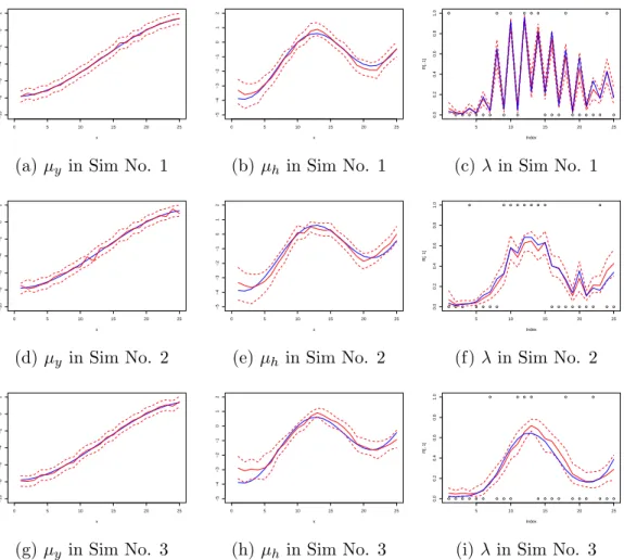
to the three sets of data. The estimation of parameters are shown in Table 2.1; plots of latent process are shown in Figure 2.2. The model correctly identified the values of

autocorrelation θψ and the association parameter φ. Moreover, the nonlinear latent

hierarchiesµy andµh were both accurately estimated. The hazard function estimates

(30)

the true values. Therefore, we conclude that our JHGP model is robust to different parametrizations.

Sim No. (true values) θψ φ

Sim 1 (θψ =−0.8,φ = 0.9) -0.77 (-0.81,-0.74) 0.86 (0.69, 1.04)

Sim 2 (θψ =−0.5,φ =−0.3 ) -0.53 (-0.48,-0.57) -0.28 (-0.44, -0.12)

Sim 3 (θψ =−0.1,φ = 0.01 ) -0.09 (-0.14,-0.02) 0.03 (-0.10, 0.18)

Table 2.1: Estimation of parameters with different (θψ, φ). The posterior means (with

95% credible intervals) are shown.

0 5 10 15 20 25 −10 −8 −6 −4 −2 0 2 x

(a) µy in Sim No. 1

0 5 10 15 20 25 −5 −4 −3 −2 −1 0 1 2 x (b)µh in Sim No. 1 ● ●●●●●● ● ● ● ● ●●● ●●● ● ●●●●● ● ● 5 10 15 20 25 0.0 0.2 0.4 0.6 0.8 1.0 Index R[, 1] (c) λin Sim No. 1 0 5 10 15 20 25 −10 −8 −6 −4 −2 0 2 x (d)µy in Sim No. 2 0 5 10 15 20 25 −5 −4 −3 −2 −1 0 1 2 x

(e)µh in Sim No. 2

●●● ● ●●●● ●●●●●●● ●●●●●●● ● ●● 5 10 15 20 25 0.0 0.2 0.4 0.6 0.8 1.0 Index R[, 1] (f)λin Sim No. 2 0 5 10 15 20 25 −10 −8 −6 −4 −2 0 2 x (g) µy in Sim No. 3 0 5 10 15 20 25 −5 −4 −3 −2 −1 0 1 2 x (h)µh in Sim No. 3 ●●●●●● ● ●●● ●●● ●●●● ● ●●● ● ●●● 5 10 15 20 25 0.0 0.2 0.4 0.6 0.8 1.0 Index R[, 1]

(i)λin Sim No. 3

Figure 2.2: Estimation of the latent processes using JHGP model in simulation stud-ies. The true unknown processes are shown in blue, and the estimated values and the 95% pointwise credible intervals are shown in red.

(31)

2.3.2 Choice of Covariance Function for Individual Process

The choice of covariance function affects the behavior of extrapolation curve. In

the population hierarchy estimates (µ), the results do not seem to differ much by

covariance selection (except for differentiabilities). On the individual level (Yi and

Hi), the basic properties of the chosen covariance function are directly exhibited its

prediction mean.

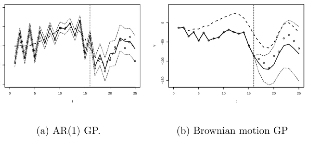
We conducted a simple comparison between a stationary and non-stationary co-variance function . As shown in Figure 2.3, the stationary AR(1) process with a

negative θψ tends to oscillate around the mean. This property is useful if the subject

trajectory is expected to progress similarly to other. On the other hand, Brownian motion as a martingale process always shows a constant difference from the mean process. This can reflect the notion that a loss or gain at a certain time is permanent for an individual. Such properties can be used together by choosing the sum of two different covariances. ● ● ● ● ● ● ● ● ● ● ● ● ● ● ● ● ● ● ● ● ● ● ● ● ● 0 5 10 15 20 25 −100 −50 0 50 100 t Y (a) AR(1) GP. ●● ● ● ● ● ●● ● ● ● ●●● ● ● ● ● ● ● ● ● ● ● ● 0 5 10 15 20 25 −150 −100 −50 0 t Y (b) Brownian motion GP

Figure 2.3: Different types of covariance functions in the individual process leads to different extrapolation curves (solid lines on the right).

2.3.3 Signal Detection of Association

In the JHGP model, the association between two responses is established by the

(32)

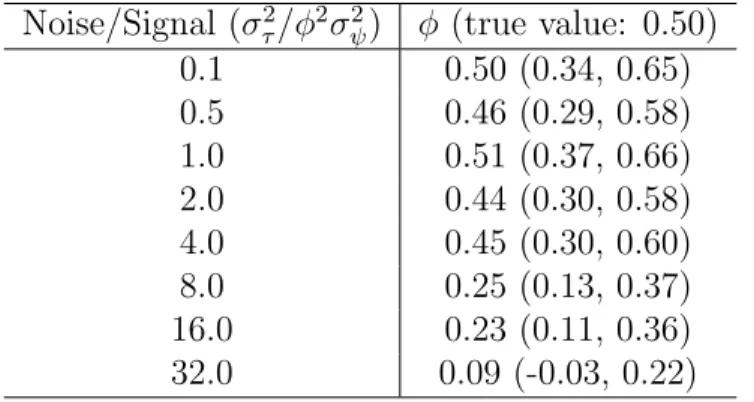
We assessed the effectiveness of φ in association detection under various levels of interference.

We use the same equations in Sec 3.1 to generate test samples withφ= 0.5, except

we add a noise vector τi ∼N(0,Iστ2) to Hi.

Hi =µh+φψi+τi

We then gradually increase σ2

τ in order to disturb the estimation ofφ. The

noise-signal ratio is controlled by σ2

τ/(φ2||σ2ψi||), where ||σ

2

ψi|| is the average of σ

2

ψi. The

results are shown in Table 2.2. The JHGP model exhibits robustness in the presence of disturbance. The numerical estimates only start to degrade around noise-signal

ratio of 8.0 yet the association remains significant until the magnitude reaches 32.0.

We conclude that the JHGP model is very robust in detecting the association between two responses.

Table 2.2: Association measures under different noise levels

Noise/Signal (σ2 τ/φ2σ2ψ) φ (true value: 0.50) 0.1 0.50 (0.34, 0.65) 0.5 0.46 (0.29, 0.58) 1.0 0.51 (0.37, 0.66) 2.0 0.44 (0.30, 0.58) 4.0 0.45 (0.30, 0.60) 8.0 0.25 (0.13, 0.37) 16.0 0.23 (0.11, 0.36) 32.0 0.09 (-0.03, 0.22) 2.3.4 Sensitivity-Specificity Studies

We conduct sensitivity analysis on the survival part of the JHGP model. We compare the results using JHGP, HGP and simple logistic regression. The posterior

(33)

means of λi are used as the fitted probabilities in the first two models. As shown in

Figure 2.4, the JHGP model has largest area under curve measure (AU C = 82.8%),

while the HGP model is weaker (AU C= 78.2%). This supports the notion that joint

modeling provides better estimation for the hazards. The least favorable model is the

simple logistic regression (AU C = 62.6%), in which Yi is treated as a covariate.

1−Specificity Sensitivity 0.0 0.2 0.4 0.6 0.8 1.0 1.0 0.8 0.6 0.4 0.2 0.0

Figure 2.4: Sensitivity-specificity analyses in simulation studies. From up-left to the diagonal, ROC curves (AUC) of model fitted with: JHGP (0.828), extended HGP(0.782), logistic regression (0.626).

2.3.5 Forecasting Performance

We censor each subject in the simulated data using random timeCi = min(max(Xi), tc)

where tc ∼ U(0,2 max(Xi)) and max(Xi) is the last recorded time in that subject.

This mechanism results in censoring in about 50% of the subjects, for which censoring occurs at random time points.

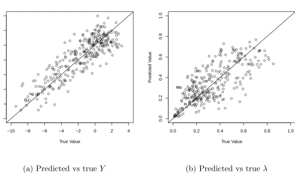
The assessment of the forecasting performance is presented in Table 2.3 and illus-trated in Figure 2.5. The model shows high prediction precision, low bias and small prediction error. The predicted values are highly correlated to the true values.

(34)

● ● ● ● ● ● ● ● ● ● ● ● ● ● ● ● ● ● ● ● ● ● ● ● ● ● ● ● ● ● ● ● _● ● ● ● ● ● ● ● ●● ● ● ● ● ● ● ● ● ● ● ● ● ● ● ● ● ● ● ● ● ● ● ● ● ●● ● ● ● ● ● ● ● ● ● ● ● ● ● ● ● ● ● ● ● ● ● ● ● ● ● ● ● ● ● ● ● ● ● ● ● ● ● ● ● ● ● ● ● ● ● ● ● ● ●_● ● ● ● ● ● ● ● ● ● ● ● ● ● ● ● ● ● ● ● ● ● ● ● ● ● ● ● ● ● ● ● ● ● ● ● ● ● ● _● ● ● ● ● ● ● ● _● ● ● ● ● ● ● ● ● ● ● ● ● ● ● ● ● ● ● ● ● ● ● ● ● ● ● ● ● ● ● ● ● ● ● ● ● ● ● ● ● ● ● ● ● ● ● ● ● ● ● ● ● ● ● ● ● ● ● ● ● ● ● ● ● ● ● ● ● ● ● ● ● ● ● ● ● ● ● ● ● ● ● ●●● ● ●● ● ● ● ● ● ● ● ● ● ● ● ● ● ● ● ● ● ● ● ● ● ● ● ● ● ● ● ● ● ● ● ● ● ● ● ● ● ● ● ● −10 −8 −6 −4 −2 0 2 4 −10 −8 −6 −4 −2 0 2 4 True Value Predicted V alue

(a) Predicted vs trueY

● ● ● ● ● ● ● ● ● ● ● ● ● ● ● ● ●●● ● ● ● ● ● ● ● ● ● ● ● ● ● ● ● ● ● ● ● ● ● ● ● ● ● ● ● ● ● ● ● ● ● ● ● ● ● ● ● ● ● ● ● ● ● ● ● ● ● ● ● ● ● ● ● ● ● ● ● ● ● ● ● ● ● ● ● ● ● ● ● ● ● ● ● ● ● ● ● ● ● ● ● ● ● ● ● ● ● ● ● ● ● ● ● ● ● ● ● ● ● ● ● ● ● ● ● ● ● ● ● ● ● ● ● ● ● ● ● ● ● ● ● ● ● ● ● ● ● ● ● ● ● ● ● ● ● ● ● ● ● ● ● ● ● _● ● ● ● _● ● ● ● ● ● ● ● ● ● ● ● ● ● ● ● ● ● ● ● ● ● ● ● ● ● ● ● ● ● ● ● ● ● ● ● ● ● ● ● ● ● ● ● ● ● ● ● ● ● ● ● ● ● ● ● ● ● ● ● ● ● ● ● ● ● ● ● ● ● ● ● ● ● ● ● ● ● ● ●●● ● ● ● ● ● ● ● ● ● ● ● ● ● ● ● ● ● ● ● ● ● ● ● ● ● ● ● ● ● ● ● ● ● ● ● ● ● ● ● ● ● ● ● 0.0 0.2 0.4 0.6 0.8 1.0 0.0 0.2 0.4 0.6 0.8 1.0 True Value Predicted V alue (b) Predicted vs trueλ

Figure 2.5: Forecasting performance in simulation studies. Comparison plots of the predicted vs the true values.

Y λ

MPSD 0.25 0.19

MAD 0.64 0.30

RMSE 0.52 0.71

Cor 0.86 0.73

Table 2.3: Forecasting performance of JHGP model in simulation studies. Mean posterior standard deviation (MPSD), median absolute deviation (MAD), Root Mean

Square Error (RMSE) and Pearson correlation (Cor) are shown. The first three

metrics are shown in relative magnitudes, as compared with absolute posterior mean, median absolute value and standard deviation.

(35)

2.4 Application in Medical Monitoring

The JHGP model is now applied to the motivating clinical problem. Percentage of

forced expiratory volume in 1 second (FEV1%) is a common measure of lung function

in cystic fibrosis (CF) patients. Studies have demonstrated that the rates of change

differ in adolescence and adulthood (VandenBranden, McMullen, Schechter, Pasta,

Michaelis, Konstan, Wagener, Morgan, and McColley, 2012) and the decline of is

nonlinear(Szczesniak, McPhail, Duan, Macaluso, Amin, and Clancy, 2013).

Pul-monary exacerbation (PEx) is a temporary worsening of lung condition due to in-fection or inflammation and can occur multiple times in an individual CF patient. Therefore PEx needs be modeled as a recurrent survival event. A previous study has

also established an association between PEx and subsequent FEV1% decline (Sanders,

Bittner, Rosenfeld, Redding, and Goss, 2011). Patient-specific maximum quarterly

FEV1% and occurrence of PEx are used for the analysis. Data were acquired from the

Cystic Fibrosis Foundation Patient Registry. The quarterly ages are used as the time indices for the discrete model. Among patients who have experienced both PEx and

FEV1% decline, we selected a sample of 38 subjects with 818 entries of observation.

Then, the more recent 50% of observations (both FEV1% and PEx) are masked in 19

randomly chosen subjects. This subset results in a training and testing split of about 75% and 25%, respectively.

We first focus on the parameter estimation.The JHGP model detects a strong

autocorrelation (θψ = −0.82) in the shared Gaussian process ψ; the variations of

FEV1% and PEx hazard has a negative correlation (φ = −0.11). It is worth

men-tioning that the estimate ofφ indicates a strong association. The small magnitude is

due to the fact that the FEV1% has its mean around 70, while hazards are commonly

limited to (−10,10) under logit link. One possible way to increase the sensitivity of

this parameter is to standardizeY before fitting the model; however, we kept FEV1%

(36)

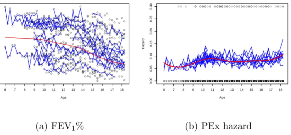
hazard are shown in Figure 2.6. The mean smoother and individual AR(1) processes are satisfactorily estimated. Among which, the population estimates are consistent

with what we found in an earlier study using penalized splines (Szczesniak, McPhail,

Duan, Macaluso, Amin, and Clancy, 2013). The baseline hazard has smooth esti-mates yet does not resemble any common parametric distribution, which indicates the flexibility in the Gaussian process. The stochasticity of individual variation in the PEx hazard is also captured by the JHGP model, due to the significant value of

φ. Caution is needed to assess the hazard function estimates at the two ends, where

data are sparse and the estimation may be biased.

We next analyze the forecasting performance of the JHGP model in FEV1%. The

validation metrics are shown in Table 2.4. Overall, the JHGP model shows high precision and low bias in forecasting (Figure 2.7). We further dissect the results and study the effects of the two hierarchies. The population Gaussian process seems adequate for predicting the future trend; however, the accuracy is further improved with the second individual process. Besides the better metrics, the improvement is illustrated in Figure 2.8, where AR(1) process captures more details in the data.

Lastly, we study the sensitivity of the survival submodel in the JHGP. Simi-lar to the simulation studies, we compare the ROC plot of the JHGP model with

the extended HGP model and the simple logistic model with F EV1% as a covariate

(Figure 2.9). The JHGP and extended HGP models show clear advantage over the traditional logistic model, probably due to their nonparametric nature. The consid-eration of joint modeling also boosts the sensitivity in comparison between the JHGP and extended HGP.

(37)

Age FEV1% 20 40 60 80 100 120 6 7 8 9 10 11 12 13 14 15 16 17 18 (a) FEV1% Age Hazard 0.00 0.05 0.10 0.15 0.20 0.25 0.30 6 7 8 9 10 11 12 13 14 15 16 17 18 (b) PEx hazard

Figure 2.6: Fitted values of FEV1% and PEx hazard with JHGP model on CF data

Population GP JHGP

MPSD - 5.46

MAD 8.66 6.43

RMSD 10.63 8.47

Cor 0.89 0.93

Table 2.4: Forecasting performance in FEV1% using JHGP model. To show the

improvement of prediction from the individual hierarchy, the metrics of the population Gaussian process is also listed. The metrics are mean posterior standard deviation (MPSD), median absolute deviation (MAD), root mean square error (RMSE) and Pearson correlation (Cor) are shown. The metrics are shown in absolute magnitudes.

● ● ● ● ● ● ● ● ● ● ● ● ● ● ● ● ● ● ● ● ● ● ● ●● ● ● ● ● ● ● ● ● ● ● ● ● ● ● ● ● ● ● ● ● ● ● ● ● ● ● ● ● ● ● ● ● ● ● ● ● ● ● ● ●● ● ● ● ● ● ● ● ● ● ● ● ● ● ● ● ● ●● ● ● ● ● ● ● ● ● ● ● ● ● ● ● ● ● ● ● ● ● ●● ● ● ● ● ● ● ● ● ● ● ● ● ● ● ● ● ● ● ● ● ● ● ● ●● ● ● ● ● ● ● ● ● ● ●● ● ●● ● ●● ● ● ● ● ● ●● ● ● ● ● ● ● ● ● ● ● ●● ● ● ● ●● ● ● ● ●● ● ●● ● ● ● ● ● ● ● ● ● ● ● ● ● ● ● ● ● ● ● ●● ● ● ● ● ● ● ● ● ● ● ● ● ● ● ● ● ● ● ● ● ●● ● ● ● ● ●● ● ● ● ●● ● ● ● ● ● ● ● ●● ● ● ● ● ● ●● ● ● ● ● ● ● ● ● ● ● ● ● ●● ● ● ● ● ● ●●●● ● ● ● ● ● ●● ● ● ● ● ● 20 40 60 80 100 20 40 60 80 100 True Value Predicted V alue

Figure 2.7: Forecasting performance in FEV1% of CF data. Comparison plots of the

(38)

● ● ● ●● ● ● ● ● ●● ● ● ● ● ● ● ● ● ●● ● ● ● ● ● Age FEV1% 45 50 55 60 65 6 7 8 9 10 11 12 13

Figure 2.8: Forecasting in FEV1% using two hierarchies of Gaussian process. The

population smoothed line (adjusted with individual intercept) are shown in red; and individualized AR(1) prediction is shown in blue. The 95% credible intervals are also included. 1−Specificity Sensitivity 0.0 0.2 0.4 0.6 0.8 1.0 1.0 0.8 0.6 0.4 0.2 0.0

Figure 2.9: ROC curves of fitting using CF data: JHGP (blue) shows higher AUC at 0.735, followed by extended HGP (red 0.683) and simple logistic regression (black 0.605).

(39)

2.5 Conclusion and Discussion

We propose a novel hierarchical model that aims to accommodate the needs of subject forecasting. As a nonparametric approach, Gaussian process modeling has several advantages over traditional methods such as spline-based approaches. Most notably, the use of covariance function instead of knots enables automatic and

ro-bust estimation. This method has been widely used in machine learning (Rasmussen

and Williams, 2006) and spatial statistics (Cressie, 1988). We further improve the Gaussian process approach with a two-hierarchy design: the first smooth Gaussian process describes the overall progression of data; the second stochastic Gaussian pro-cess captures the finer and personalized variation. The hierarchical design is not only conceptually clear, but also in alignment with one of the goals in longitudinal analysis: combining information from the levels of population and individuals.

As a predictive model, the JHGP shows high accuracy in the results of forecasting. We provide a flexible framework to incorporate the similarity in longitudinal data

and the self-memory in time series analysis. The AR(1) structure can be easily

replaced with more complex structures, as long as the covariance matrix can be derived. One possible issue may be the restriction on the positive definiteness of the covariance, however, since the population matrix is positive definite and has larger magnitude, this restriction may be lifted after adding the two variance matrices after reparameterization.

As a joint model, the JHGP adopts the individual fluctuations as the shared parameter. From the view of survival modeling, this parameter can be treated as the time-dependent frailty. We show that this design is robust to noise perturbation and also increases the sensitivity-specificity measure.

We have developed a fully Bayesian solution to the computation problem of the proposed model. Major progress has been made on Bayesian Gaussian process models

(40)

2001) (Daniels and Kass, 1999) and dimension reduction (Banerjee, Dunson, and Tokdar, 2013). On the other hand, there is less attention on the hierarchical use of Gaussian processes, especially using multiple Gaussian process simulatenously. One of the relevant works in this field is the use of finite mixtures of Gaussian processes (Shi, Murray-Smith, and Titterington, 2005). Our hierarchical model differs in the sense that it is an additive model instead of a mixture model; therefore, we focus on controlling the scales of different components through prior conditioning. The shrinkage effects of g-priors and the coupling of the smaller Gaussian process with noise enables correct estimation of the latent components.

(41)

CHAPTER III

Bayesian Ensemble Trees in the Analyses of

Heterogeneous Data

In this chapter, we propose a novel “tree-averaging” model that utilizes the ensem-ble of classification and regression trees (CART). Each constituent tree is estimated with a subset of similar data. We treat this grouping of subsets as Bayesian ensem-ble trees (BET) and model them as an infinite mixture Dirichlet process. We show that BET adapts to data heterogeneity and accurately estimates each component. Compared with the bootstrap-aggregating approach, BET shows improved predic-tion performance with fewer trees. We develop an efficient estimating procedure with improved sampling strategies in both CART and mixture models. We demonstrate these advantages of BET with simulations, classification of breast cancer data and regression of lung function measurements from cystic fibrosis patients.

3.1 Introduction

Classification and regression trees (CART) (Breiman, Friedman, Olshen, and

Stone, 1984) is a nonparametric learning approach that provides fast partitioning of data through the binary split tree and an intuitive interpretation for the relation between the covariates and outcome. Aside from simple model assumptions, CART

(42)

is not affected by potential collinearity or singularity of covariates. From a statis-tical perspective, CART models the data entries as conditionally independent given the partition, which not only retains the likelihood simplicity but also preserves the nested structure.

Since the introduction of CART, many approaches have been derived with better

model parsimony and prediction. The Random Forests model (Breiman, 2001)

gener-ates bootstrap estimgener-ates of trees and utilizes the bootstrap-aggregating (“bagging”)

estimator for prediction. Boosting (Friedman, 2001, 2002) creates a generalized

ad-ditive model of trees and then uses the sum of trees for inference. Bayesian CART (Denison, Mallick, and Smith, 1998;Chipman, George, and McCulloch, 1998) assigns a prior distribution to the tree and uses Bayesian model averaging to achieve better

estimates. Bayesian additive regression trees (BART, Chipman, George, McCulloch

et al.(2010)) combine the advantages of the prior distribution and sum-of-trees struc-ture to gain further improvement in prediction.

Regardless of the differences in the aforementioned models, they share one prin-ciple: multiple trees create more diverse fitting than a single tree; therefore, the combined information accommodates more sources of variability from the data. Our design follows this principle.

We create a new ensemble approach called the Bayesian Ensemble Trees (BET) model, which utilizes the information available in the subsamples of data. Similar to Random Forests, we hope to use the average of the trees, of which each tree achieves an optimal fit without any restraints. Nonetheless, we determine the subsamples through clustering rather than bootstrapping. This setting automates the control of the number of trees and also adapts the trees to possible heterogeneity in the data.

In the following sections, we first introduce the model notation and its sampling algorithm. We illustrate the clustering performance through three different simulation settings. We demonstrate the new tree sampler using homogeneous example data from

(43)

a breast cancer study. Next we benchmark BET against other tree-based methods using heterogeneous data on lung function collected on cystic fibrosis patients. Lastly, we discuss BET results and possible extensions.

3.2 Preliminary Notation

We denote theith record of the outcome asYi, which can be either categorical or

continuous. EachYi has a corresponding covariate vector Xi.

In the standard CART model, we generate a binary decision tree T that uses

only the values of Xi to assign the ith record to a certain region. In each region,

elements ofYi are identically and independently distributed with a set of parameters

θ. Our goals are to find the optimal treeT, estimate θ and make inference about an

unknown Ys given values of Xs, wheres indexes the observation to predict.

We further assume that {Yi,Xi} is from one of (countably infinitely) many trees

{Tj}j. Its true origin is only known up to a probability wj from the jth tree.

There-fore, we need to estimate bothTj andwj for eachj. Since it is impossible to estimate

over all j’s, we only calculate those j’s with non-negligiblewj, as explained later.

3.3 Bayesian Ensemble Tree (BET) Model

We now formally define the proposed model. We use [.] to denote the probability

density. Let [Yi|Xi,Tj] denote the probability of Yi conditional on its origination

from the jth tree. The mixture likelihood can be expressed as:

[Yi|Xi,{Tj}j] =

∞

X

j

wj[Yi|Xi,Tj] (3.1)

where the mixture weight vector has an infinite-dimension Dirichlet distribution with

precision parameterα: W={wj}j ∼Dir∞(α). The likelihood above corresponds to

Yi iid

(44)

G is simply the binary tree [Yi|Tj].

3.3.1 Hierarchical Prior for T

We first define the nodes as the building units of a tree. We adopt the notation

introduced by Wu, Tjelmeland, and West (2007) and use the following method to

assign indices to the nodes: for any nodek, two child nodes are indexed as left (2k+1)

and right (2k+ 2); the root node has index 0. The parent of any nodek >0 is simply

bk−1

2 c, where b.c denotes the integer part of a non-negative value. The depth of a

nodei is blog₂(k+ 1)c.

Each node can have either zero (not split) or two (split) child nodes. Conditional

on the parent node being split, we use sk = 1 to denote one node being split (or

interior), sk = 0 otherwise (or leaf). Therefore, the frame of a tree with at least one

split is:

[s0 = 1]

Y

k∈Ik

[s2k+1|sk = 1][s2k+2|sk= 1]

where Ik ={k:sk= 1}denotes the set of interior nodes.

Each node has splitting thresholds that correspond to the m covariates in X. Let

them−dimensional vectortkdenote these splitting thresholds. Also, it has a random

draw variable ck from {1, ..., m}. We assume sk,tk, ck are independent.

For the ckth element X(ck), if X(ck) < t(ck), then observation i is distributed to its

left child; otherwise it is distributed to the right child. For every i, this distributing

process iterates from the root node and ends in a leaf node. We useθk to denote the

distribution parameters in the leaf nodes. For each node and a complete tree, their prior densities are:

[Tk] = [sk][ck]sk[tk]sk[θk]1−sk [T] = [T0] Y k∈Ik [T2k+1][T2k+2] (3.2)

(45)

For sk,tk, ck, we specify the prior distributions as follows:

sk ∼B(exp(−blog2(k+ 1)c/δ))

ck ∼M Nm(ξ), where ξ ∼Dir(1m)

[tk]∝1

(3.3)

where B denotes a Bernoulli distribution, M Nm is an m-dimensional multinomial

distribution. The hyper-parameterδis the tuning parameter for which smaller values

of δ result in smaller trees.

In each partition, objective priors are used for θ. If Y is continuous, then [θk] =

[µ, σ2]∝1/σ2; ifYis discrete, thenθk =p ∼Dir(0.5·1). Note thatDirreduces to a

Betadistribution when Y is a binary outcome. To guarantee the posterior propriety

of θ, we further require that each partition should have at least q observations and

q >1.

The posterior distribution of ξ reveals the proportion of instances that a certain

variable is used in constructing a tree. One variable can be used more times than

another, therefore resulting in a larger proportion in ξ. Therefore, ξ can be utilized

in variable selection and we name it as variable ranking probability.

3.3.2 Stick-Breaking Prior for W

The changing dimension of the Dirichlet process creates difficulties in Bayesian sampling. Pioneering studies include exploring infinite state space with the

reversible-jump Markov chain Monte Carlo (Green and Richardson, 2001) and with an

auxil-iary variable for possible new states (Neal, 2000). At the same time, an equivalent

construction named the stick-breaking process (Ishwaran and James, 2001a) gained

popularity for its decreased computational burden. The stick-breaking process

(46)

w1 =v1 wj =vj Y k<j (1−vk) for j >1 (3.4) where eachvj iid

∼ Beta(1, α). This construction provides a straightforward illustration

of the effects of adding/deleting a new cluster to/from the existing clusters.

Another difficulty in sampling is that j is infinite. Ishwaran and James (2001a)

demonstrated that the max(j) can be truncated to 150 for a sample size of n = 105_,

and the results are indistinguishable from those obtained using larger numbers. Later,

Kalli, Griffin, and Walker (2011) introduced the slice sampler, which avoids the

approximate truncation. Briefly, the slice sampler adds a latent variableui ∼U(0,1)

for each observation. The probability in (3.1) becomes:

[Yi|Xi,{Tj}j] =

∞

X

j

1(ui < wj)[Yi|Xi,Tj] (3.5)

due toR₀11(ui < wj)dui =wj. The Monte Carlo sampling ofui leads to omittingwj’s

that are too small. We found that the slice sampler usually leads to a smaller effective maxj <10 for n= 105_{, hence more rapid convergence than a simple truncation.}

3.4 Blocked Gibbs Sampling

We now explain the sampling algorithm for the BET model. LetZi =jdenote the

latent assignment of the ith observation to the jth tree. Then the sampling scheme

for the BET model involves iteration over two steps: tree growing and clustering.

3.4.1 Tree Growing: Updating [T|W,Z,Y]

Each tree with allocated data is grown in this step. We sample in the order of

(47)

using [Y|s,c,t] marginalized over θ facilitates rapid change of the tree structure.

After the tree is updated, the conditional sampling of θ provides convenience in the

next clustering step, where we compute [Yi|Tj] for different j.

During the updating of [s,c,t], we found that using a random choice in the

grow/prune/swap/change (GPSC) in one Metropolis-Hastings (MH) step (Chipman,

George, and McCulloch, 1998) is not sufficient to grow large trees for our model. This is not a drawback of the proposal mechanism, but is instead primarily due to the notion that following this clustering process would distribute the data entries to many small trees, if any large tree has not yet formed. In other words, the goal is to have our model prioritize “first in growing the tree, second in clustering” instead of the other order.

Therefore, we devise a new Gibbs sampling scheme, which sequentially samples the full conditional distribution [sk|(sk)], [ck|(ck)] and [tk|(tk)]. For each update, MH

criterion is used. We restrict updates of c,t that result in an empty node such that

s will not change in these steps. The major difference in this approach compared

to the GPSC method is that, rather than one random change in one random node, we use micro steps to exhaustively explore possible changes in every node, thereby increasing chain convergence.

Besides increasing the convergence rate, the other function of the Gibbs sampler is to force each change in the tree structure to be small and local. Although some

radical change steps (Wu, Tjelmeland, and West, 2007;Pratola, 2013) can facilitate

the jumps between the modes in a single tree, for a mixture of trees, local changes and mode sticking are useful to prevent label switching.

3.4.2 Clustering: Updating [W,Z|T,Y]

In this step, we take advantage of the latent uniform variable U in the slice