Agriculture
Haluk Gedikoglu and Joseph L. Parcell
This research analyzes factors affecting product and profi t lifecycles for new value-added products. The methodology presented shows how sales and profi ts evolve and how exogenous factors such as initial marketing efforts affect sales and profi ts. Results indicate that producers can increase the level of profi ts over time through initial marketing efforts. The theoretical model is applied to a quality cattle program to assess the analytical performance of the model.
Gedikoglu is Associate Lecturer, Department of Economics, University of Wisconsin-La Crosse. Parcell is Associate Professor, Department of Agricultural Economics, University of Missouri-Columbia.
Value-added agriculture stems from using a commodity to produce a product that is either a complement to or substitute for an existing end-use or industrial product. Sometimes the product is dif-ferentiated very little (e.g., ethanol) and other times the product displays signifi cant differentiation (e.g., Blue Diamond Almonds). Most of the economic questions surround the signifi cantly differentiated value-added products. The most important ques-tions are, “How profi table will the new product be?” and, “How long will the profi t stream last?” General wisdom is that the profi t stream will shorten as competition arises. The objective of this study is to show, through comparative dynamics, the value to agricultural producers of initial marketing efforts of extending a product’s lifecycle.
Product-lifecycle theory is widely used in the marketing-strategy literature to evaluate the ex-pected sales and profi t levels for new products or a product-line extension. The theory predicts that profi ts will increase as sales increase. They will then reach a maximum, after which profi ts will trend to zero because of competitive factors. However, certain choices and actions can change the length of the product lifecycle, most importantly the period for which profi ts are positive. These factors include initial marketing efforts (delay factor), the time at which profi ts obtain the maximum (infl ection point), and the projected sales ceiling.
The results of the current research are directly applicable to value-added businesses seeking a competitive advantage during startup. Furthermore, this research can be used to emphasize the need for adequate initial working capital.
Theoretical Model
The product-lifecycle approach has been used to analyze and forecast sales and profi t levels. Cox (1967) showed that the lifecycle of a new product is characterized by four stages: introduction, growth, maturity, and decline. The introduction stage is when the product is fi rst marketed and sales are less than fi ve percent of the market share. During this period, profi ts improve from negative to posi-tive. In the growth phase, sales volume increases rapidly, and positive profi ts continue to increase. The growth phase ends with profi ts reaching the maximum level. The next phase is the maturity phase, in which both the rate of increase in sales volume and profi ts plateau and begin to decline. The last phase is the decline stage. During the decline phase, both total sales and profi ts decline rapidly. Figure 1 shows the stages of the product lifecycle (Cox 1967) and Figure 2 shows the corresponding profi t lifecycle. In the literature, the profi t lifecycle is obtained implicitly from the product lifecycle, but an analytical framework for the profi t lifecycle is missing. As the decline stage is economically undesirable, the current study does not take into account this stage.
The formulation of the product lifecycle model is (Cox 1967) (1)
F
S
e
tF
tF
=
A I+
1
A IA I t(((( −−t)))) for t = 1,2…Tfor t = 1,2…Tfor t = 1,2…T,,where ttt is the index for time, is the index for time, Fttt is the cumulative is the cumulative sales level at time t, SSS is the saturation (maximum) is the saturation (maximum) level of sales, T T T is the time at which cumulative is the time at which cumulative sales reach the saturation level of sales and I is the infl ection point and the time at which profi ts reach the maximum—the beginning of the maturity phase.
Note: Vertical axis values for presentation purposes only. Figure 1. Product Lifecycle Example.
0
5000
10000
15000
20000
25000
1
2
3
4
5
6
7
8
9
10
11
12
Year Cumulative Sale sI
IntroductoryPhase Growth Phase
S T Maturity Phase -$100 -$50 $0 $50 $100 $150 $200 1 2 3 4 5 6 7 8 9 10 11 12 Year
Profits
IntroductoryPhase Growth Phase Maturity Phase
T
I
Note: Vertical axis values for presentation purposes only. Figure 2. Profi t Lifecycle Example.
1 Appendix information that shows the derivation of the result
is available from authors upon request.
2 Figure 2 shows the profi t curve for Figure 2 shows the profi t curve for Figure 2 shows the profi t curve for = 21000, S S A = 1, III = 7, = 7,
and T = 12.
sales of a product will stay in the introductory phase
(
A
∈
[ , ]
0 1
). A value of A close to one indicates along introductory phase, whereas a value close to zero indicates a short introductory phase. A short introductory phase is desirable in that it allows positive profi ts to be rapidly obtained. In general, marketing efforts in the introductory phase cause
A to approach zero (Morrison 1995).
Morrison (1995) graphically presented the effect of a change in the levels of S, III, and , and A on the prod-uct lifecycle. However, the analytical framework to analyze the effect of these changes simultaneously on the product lifecycle or Fttt was missing. The pres- was missing. The pres-ent study provides the analytical framework to show how changes in S, III, and , and A simultaneously affect the shape of the product-lifecycle curve.
The change in FFF due to a change in due to a change in A can be represented as (2)
dF S A I A t A
dA
S
dS
dA
t tdF
t tdF S A
ttttttttttttttttttttttttttttttt( (
( (
( (
( (
S A
S A
S A
S A
S A
S A I A
S A
),
),
I A
I A
I A t A
I A
I A
I A
I A
( )
( )
( )
( )
, ,
, ,
, ,
, ,
t A
t A
t A
t A
t A
t A
t A
)
)
)
)
)
)
)
)
)
)
)
)
=
=
∂
∂
∂
∂
∂
F
F
F
F
F
F
F
F
F
F
F
F
F
F
F
F
F
F
ttttttttttttttttttttttttttttttt(
(
(
(
(
(
(
(
(
(
(
(
.)
∂
+
∂
∂
+ ∂
∂
F
∂
F
∂
I
∂
I
∂
ttdA
+
+
∂
∂
ttA
A
F
t tF
tttttttttttttt(.
(.
)
)
)
)
)
)
)
)
)
)
)
dI
dI
dI
dI
dI
dI
+
+ ∂
+
+
∂
∂
∂
∂
∂
∂
∂
∂
∂
∂
∂
∂
∂
∂
∂
∂
∂
F
F
F
F
F
F
F
F
F
F
F
F
tttttttttttttt(
(
(
(
(
(
(
(
(
(
(
.)
for t = 1,2…T. for t = 1,2…T. for t = 1,2…TThe results show that for t < It < It < I F, , t(.) increases by decreasing A. However, for t > It > It > I F, , t(.) decreases by decreasing A.1
Even though sales are important for producers, and the product-lifecycle model analyzes sales, the profi ts obtained from sales determine whether com-panies continue production. The product-lifecycle model does not provide an explicit formulation for the profi t function. However, we show how initial marketing efforts affect profi ts.
Profi t Lifecycle
To observe the change in the level of profi ts at each period, the profi t function is specifi ed as2
(3)
π
tF S
F S
tttA I A t A
t
P
P
ttt tt
∂
F S
∂
F S
∂
= ∂
∂
−
( (
F S
( (
F S
A I
A I
),
),
( )
( )
A t
A t
A t
A t
, ,
, ,
)
)
)
)
)
)
P F
P
F
F
F
tttttt(
(
(
(
(
(
)
(
∂
)
∂
∂
F
F
(
)
∂
F
F
(
.)
c A b F
t
tF
tF
( )
c A
( )
c A
− ∂
∂
F
F
(.)
∂
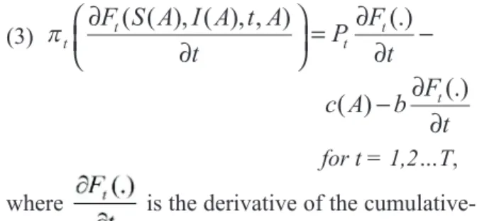
for t = 1,2…T, for t = 1,2…T, for t = 1,2…Twhere is the derivative of the cumulative-lifecycle function with respect to t, which gives the instantaneous sales amount at time t, while Pttt is the is the price of the product at time t. A linear cost function is assumed with respect to an instantaneous sales level in which b is the slope and c(A) the intercept. The term c(A) includes the initial marketing cost and fi xed production costs, which implies , as marketing efforts refl ect a decrease in A. We as-sume c(A) does not trend over time and is only af-fected by A, where A can only be altered during the introductory phase. The effect of a change in A on the level of profi ts attained in each period is3
(4) ∂ ∂ = + ∈ − ∈
{
}
πt A ∂A ∂(.) ++−+−+ for t for t/-/- for t for t∈∈∈∈∈∈
{
{
{
{
{
{
{
{
{
{
Introductorytroductorytroductory Phase Phase}
}
}
}
}
}
}
}
}
}
for t{
Gr}
{
Grrowth P}
{
Grrowth PGrrowth P}
{
Grrowth PGr hase}
{
hase}
{
Maturity}
{
Maturity Phase}
{
Maturity PhaseMaturity Phase}
{
Maturity PhaseMaturity}
−− for t for t∈∈ .The negative sign in Equation 4 indicates initial marketing efforts cause profi ts to increase for the corresponding years and the positive sign indicates a decrease in profi t due to initial marketing efforts. As the change in c(A) through initial marketing efforts occurs only in the introductory phase, profi ts are expected to be lower in the introductory phase (initial years) and higher in the years following the introduc-tory phase due to increased sales. Depending on the magnitude of the marketing costs, positive profi ts may also be realized in the introductory phase. Application of Product- and Profi t-Lifecycle Theories
The Show-Me-Select (SMS) Heifer Program of Missouri was initiated in 1997 to develop a
high-3 Appendix information that shows the derivation of the result
quality, branded, bred heifer supply—effectively creating an increased value via branding for the heif-ers. Profi tability was a crucial criterion for farmers to remain participants in this program. We use this example because of the completeness of available data to provide credence to the theoretical model.
The data needed to formulate cumulative sales and profi ts for the SMS Heifer Program was ob-tained via the documentation of SMS Heifer Pro-gram special sales, available for the 1998 through 2004 period (Patterson and Randle 2006). The data used in the simulation analysis were obtained by aggregating the information supplied by individual producers. Therefore the results more closely refl ect changes in Missouri beef industry levels. Bayus (1998) demonstrates that the length of a product lifecycle can differ for individual producers and suggests that the conclusions about the product lifecycle should be made based on industry-level data instead.
The use of the product-lifecycle method requires sales data. However, for new products a forecast of sales is the only available information. Morrison (1995) provides approximation methods for param-eters in the product lifecycle of new products. More specifi cally, an estimated version of Equation 1 can be used to arrive at (5)
F
S
e
tF
tF
A I(.)
( ) A I( ) A I t( t) ∧ ∧ ( −) ( )=
+
∧ ∧1
for t = 1,2...Tt = 1,2...Tt = 1,2...T,,where ŜŜŜ is the approximated value of the saturation is the approximated value of the saturation level of the sales volume, Â is the estimated sig-nifi cance of the delay factor, and ÎÎÎ is the projected is the projected value of the infl ection point. According to Morrison (1995), the value of ŜŜŜ is found to be the maximum is found to be the maximum cumulative amount of sales the product is expected to achieve.4
The total number of registered heifer buyers at-tending sales for 2003 was 595, the average herd size for a registered buyer was 90 animals, 61
per-cent of the registered buyers bought SMS Heifers, and 73 percent of those who bought SMS Heifers indicated they want to continue buying SMS Heifers (Parcell et al. 2005). The number of actual buyers is calculated by multiplying the total number of registered buyers (595) by the percentage of buyers who actually bought heifers (61 percent). To ap-proximate the number of future buyers, the number of actual buyers (363) is multiplied by the number of buyers who want to continue buying SMS Heif-ers (73 percent). Finally, to fi nd the expected future total sales of SMS Heifers, the average herd size (90 head) of these actual buyers is multiplied by the estimated number of future buyers, equating to ŜŜŜ = = (595 * 0.61 * 0.73) * 90, or 23,845 heifers.
The value of  and ÎÎÎ are calculated by using are calculated by using the non-linear optimization procedure from Kros (2005). Using the calculated value of Ŝ, the values for  and ÎÎÎ are selected to minimize the sum of are selected to minimize the sum of squared errors between the actual cumulative sales data and the expected value of cumulative sales for heifers in the program between 1997 and 2004. Specifi cally, (6)
min
(
,
)
. .
,
,
, ( ) A I, A I, t t A IA I(((( t))))F
tF
te
s t
. .
s t
. .
A
I
∧ ∧n
(
∧ ∧n
(
−
∧ ∧+
≤
( −) ( ) = ∧ ∧∑
n
∑
(
n
(
23 845
1
0
A
1
0
≤ ≤
A
1
0
≤ ≤
≤ ≤
A
A
1
0
≤ ≤
A
A
1
0
2 1 8where Fttt is the actual cumulative sales data for year is the actual cumulative sales data for year
t. Two constraints are assumed:  is between zero and one, and Î is positive.  is found to be 0.37. The small magnitude of  is likely due to signifi -cant initial marketing efforts for the SMS Heifer Program.5 The value of ÎÎÎ is 7.5, showing that profi ts is 7.5, showing that profi ts
for the program continued to rise for 7.5 years after the program began.
4 An example is benefi cial. Following Morrison (1995), for a
producer who wants to sell a new type of tomato in a small town, ŜŜŜ is calculated. It is known by this producer, from market is calculated. It is known by this producer, from market research, that there are 1,000 people in the town who buy tomatoes, two every year. Also, through consumer surveys it is learned that 25 percent of the potential consumers will purchase a new tomato. From the market information, the saturation level of sales is approximated ŜŜŜ = 1000 * 2 * 0.25 = 500 tomatoes. = 1000 * 2 * 0.25 = 500 tomatoes.
5 Producer-owner representatives at sale locations advertise
widely, with the University of Missouri Extension system serving as catalyst for marketing efforts. The consignment cost for each heifer marketed through registered sales ranges from $15 to $20 per animal. Most of this consignment fee goes toward marketing. In addition, the University of Missouri Extension service offered free news releases for this program because it was initiated through University of Missouri Extension monies.
The shape of the cumulative lifecycle (CLC) curve for the SMS Heifer Program is created with two different values of Â, 0.37 and 1 (Figure 3). Recall, an ÂÂÂ equal to 1 indicated no marketing effort. equal to 1 indicated no marketing effort. As can be seen from Figure 3, when Â= 1 the shape of the CLC curve is similar to the shape generally displayed in textbooks. Total sales are initially low, grow rapidly, then reach maturity. When Â= 0.37, a higher level of sales can be reached at an earlier time in the introductory phase. As an example, the level of sales for year two is compared for each value of Â. In Year Two, total sales are projected to be 2,646 heifers when Â= 0.37 and 200 heifers when Â= 1. The actual data indicate that Year Two sales were 1,844 heifers. Overall, the CLC curve is better approximated by Â= 0.37 than by Â= 1.
As can be seen in Figure 3, a decrease in A
causes both SSS and and III to increase. The increase in to increase. The increase in S
causes sales to increase for all periods, which is consistent with the fi ndings of Morrison (1995). However, Morrison (1995) did not incorporate the change in SSS as a response to a change in as a response to a change in A. For the SMS Heifer Program, the decrease in A causes the sales level to increase for Years One through Six and 13 through 19. For Years Seven through 12, sale quantities are projected to decline due to large initial marketing efforts.6
Figure 3. Comparison of Cumulative Lifecycle (CLC) of A = 0.37 versus CLC of= 0.37 versus CLC of= 0.37 versus CLC of = 1. A A
0
5000
10000
15000
20000
25000
1
2
3
4
5
6
7
8
9
10
11
12
13 14
15
16
17
18
19
Year C um ul at iv e Sa le sActual CLC Estm. CLC for A=0.37 Estm. CLC for A=1
6 If SSS can increase suffi ciently, then the level of sales may not can increase suffi ciently, then the level of sales may not
decrease for any period. This value of SSS is calculated to be 30,666 is calculated to be 30,666 for SMS Heifer Program. However, this value of SSS could not be could not be obtained even for A = 0. Hence factors other than A also need to be used to increase S. This point requires further research.
It is possible to compare the net gain in sales from a decrease in A, i.e, increased marketing ef-forts, as A goes from 1 to 0.37. For an increase in marketing efforts, the heifer sales increase 15,489 head During Years One through Six, decrease 14,929 head During Years Seven through 12, and increase 12,887 head during Years 13 through 19. Therefore the increase in cumulative sales due to enhanced marketing efforts for the 19-year period simulated is 13,447 head.
A decrease in A causes I I I to increase. By decreasing to increase. By decreasing
A from 1 to 0.37 for the SMS Heifer Program, the in-fl ection point III increased from increased from t = 6.5 to t = 7.5. Thus early marketing efforts can substantially increase the time during which profi ts will continue to rise before peaking. Overall, the fact that actual sales data for SMS Heifer Program is better approximated by the CLC for A = 0.37 instead of the traditionally thought CLC for A = 1 shows that there will be a higher num-ber of sales than expected and a longer period during which positive profi ts will be achieved.
Profi t Curve
The profi t function for the SMS Heifer Program is simulated following the cumulative lifecycle as
(7) min (.) ( ) (.) , b c, b c, t t t(. t t(.) t t ) ( ) t t ( ) t p t pt t t Ft t Ft t t t c A t t ( ) t t c A( )( ) t t c Ac A( )( )( ) b t t b t t Ft t Ft t t t ∧ ∧ − ∂F ∂F ∂ ++ ( )( )++ t + + t t ( ) t t + ( )( )+ t t + ( )+ t t + + t t ++c Ac Ac Ac A( )( )( )( )++ t t c A t t + + t t c A t t ( ) t t c A( )( ) t t + ( )( )+ t t c A( )( ) t t ( ) ∂ t t ∂ t t ∂FFt t Ft t ∂ t t Ft t t ∂ ∧ ∧ ∧ ∧
t
t t t
t
t t t
t
t t t
π
=∑
2
2
1 7 t . The values of instantaneous rate of sales for each period,∂
∂
∧F
∂
F
∂
t
tF
tF
(.)
, used in the estimation procedure are predicted from a previously estimated cumulative lifecycle for the SMS Heifer Program using the value  = 0.37. To estimate the profi t level for each year, the price level used, pt, is the average price per heifer for SMS Heifer Program sales over the seven year period, $981/head. The estimated profi t curves for A = 0.37 and A = 1 are shown in Figure 4, actual profi ts are available for seven years.Comparing the profi t curves for A = 0.37 and A
= 1 shows the effect of marketing efforts on profi ts. Initially, profi ts are lower for A = 0.37 than for A = 1. This is due to increased marketing expenditures. The profi t levels for A = 0.37 become signifi cantly
higher after Year Six. Profi ts diminish faster for A = 1. This shows that producers receive more periods of positive profi ts when initial marketing efforts are undertaken. The approximate area under the profi t curve for A = 1, over the seven-year period, is calculated to be $617/head, while the area under the profi t curve for A = 0.37 is $955/head. When yearly profi ts for both levels of A are discounted by a discount rate of eight percent, the net cumulative gain through enhanced marketing efforts turns out to be $156/head. The estimated cumulative gain is greater than the added cost incurred through a marketing campaign. While startup costs can be huge, in theory there is a greater chance of achieving profi tability sooner by investing in initial marketing. This result reinforces the need to invest in marketing early in product development.
Brand Value
The general wisdom in agriculture is that the brand value created by product differentiation will last for a very short time, as replication of an agricultural product is often easy in comparison to other indus-tries. However, we show that through marketing efforts, short-term profi tability can be increased, and the period of profi tability can be expanded. For the current study, the brand value is defi ned as the difference between the per-head profi t levels for the SMS Heifer Program and non-program commercial bred heifers:
(8) Bttt = = πππttSMSSMSSMS − − π t πt
πnon-SMSnon-SMSnon-SMS for for for for = t t 1,2, ... T1,2, ... T1,2, ... T.. πt
πt
πSMSSMSSMS and and π t πt
πnon-SMSnon-SMSnon-SMS are the profi t levels for the program are the profi t levels for the program
and non-program heifer for each period, respec-tively. The change in the brand value due to initial marketing effort can be represented as
(9)
∂
∂
= ∂
∂
− ∂
∂
−B
∂
B
∂
A
A
∂
A
A
∂
A
t∂
∂
A
∂
∂
A
A
B
tB
SMA
SMA
A
SA
A
SA
A
SMSSMA
A
SMA
A
SA
A
SMA
A
A
t SMS SMS SM SMS SMS SM t non SMSSMSSM SMS SMS SMπ
∂
π
π
t∂
π
π
tSMπ
π
SMSπ
π
SMSSMSπ
π
SMSSMπ
= ∂
∂
− = ∂
∂
π
∂
π
π
t∂
π
π
tπ
π
SMπ
π
SMπ
π
Sπ
π
Sπ
π
SMSSMπ
π
SMπ
π
Sπ
π
SMπ
π
π
SMS SMS SM t SMS SMS SM SMS SMS SMA
A
∂
A
A
∂
A
A
A
A
SMSSMSMSSMSMSSMS− =
− =
0
0
∂
∂
A
A
A
A
π
π
0
π
π
for for for = t t 1,2, ... T1,2, ... T1,2, ... T,,where
∂
∂
−π
tnon SMSSMSSM SMS SMS SMA
∂
A
∂
is equal to zero because the initialmarketing efforts for the program do not affect the profi t levels of non-program heifers. Therefore the
total change in brand value due to the initial SMS Program marketing efforts is represented as the sum of changes in program profi ts for each period:
(10) .
From Equation 10, the total increase in brand value will be equal to the total increase in profi ts between SMS Program heifers and conventional heifers. This is calculated to be $156/head. Hence by investing in marketing efforts the program increased SMS Heifer Program heifer value by $156/head.
The estimated brand value is shown in Figure 5. The positive brand value is expected to last for 8.5 years when initial marketing efforts are undertaken for the SMS Heifer Program.7 The length of run
for the brand value is extended by two years due to initial SMS Heifer Program marketing efforts. Thus initial SMS Heifer Program marketing efforts
caused the brand value to increase in terms of an immediate price premium and due to long-term market penetration.
Conclusions
This research evaluates the theoretical and empirical impact of marketing efforts on the value-added agri-culture product lifecycle. While the lifecycle meth-odology and comparative dynamics reported in the current research can be extended to non-agricultural products, the goal of the current research is to show how the application of such methodology can explain the lifecycle of value-added commodity goods.
The results indicate, through comparative dynamics, that the product lifecycle theorem is meaningful only after incorporating the impact of a change in initial marketing efforts. Thus the ability of a business entity to sustain profi ts from invest-ments in a value-added business requires signifi cant up-front investment in marketing. Through initial marketing efforts it is possible for the value-added business entity to decrease the amount of time until positive profi t is realized and extend the number of -$100 -$50 $0 $50 $100 $150 $200 $250 $300 1 2 3 4 5 6 7 8 9 10 11 12 Year Pr of its ($ /h ea d)
Actual Profits Estm. Proifts for A=0.37 Estm. Profits for A=1
Figure 4. Profi t Lifecycle for SMS Heifer Program.
7 In Figure 4, TTT is equal to 12 years for is equal to 12 years for A = 0.37 and ten years
for A = 1, which shows that positive profi ts are realized for two more years due to initial marketing efforts.
periods producing positive profi ts. Furthermore, the fi ndings of the current study indicate that allocation of monies for marketing efforts is a critical com-ponent for success, as shown with the effect of a decrease in A on sales and profi t. When the product is successful, the increase in short-term profi ts out-weighs the added marketing cost.
Finally, the product-lifecycle projection and profi t-function analysis is applied to a producer value-added quality bred heifer program. Through simulation, the estimated level of price premiums for the bred heifer program was determined to be similar to actual premiums. Thus whether for a product or a differentiated commodity, the product-lifecycle theory applied here indicates marketing efforts are critical to the long-run success of the product and its ability to garner price premiums and generate a positive profi t.
References
Bayus, B. L. 1998. “An Analysis of Product Life-times in a Technologically Dynamic Industry.” Figure 5. Brand Value for SMS Heifer Program.
-$100
-$50
$0
$50
$100
$150
$200
$250
$300
1
2
3
4
5
6
7
8
9
Year Pr em iu m ( $ / h ea d )Actual Premium Estimated Premium for A=0.37
Management Science 44(6):763−775.
Cox, W. E., Jr. 1967. “Product Lifecycles as Mar-keting Models.” The Journal of Business 40(4): 375−384.
Kros, J. F. 2005. “Forecasting New Products with a Non-Cumulative Logistic Growth Model: A Case Study of Modem Technology.” Journal of Business Forecasting 24(1):23−32.
Business Forecasting 24(1):23−32.
Business Forecasting
Morrison, J. S. 1995. “Lifecycle Approach to New Product Forecasting.” The Journal of Business Forecasting Methods & Systems 14(2):3−5. Parcell, J. L., M. Cox, D. Patterson, and R.
Randle. 2005. “Buyer Perceptions and Willingness−to−Pay for Bred Heifer Character-istics.” Unpublished Working Paper, University of Missouri-Columbia.
Patterson, D. J. and R. F. Randle. 2006. “Missouri Show-Me-Select Economic Analysis and Sum-mary Information.” http://agebb.missouri.edu/ select/econsum.htm. Accessed November 2006.