Archive University of Zurich Main Library Strickhofstrasse 39 CH-8057 Zurich www.zora.uzh.ch Year: 2018
Tensor Algorithms for Advanced Sensitivity Metrics Ballester-Ripoll, Rafael ; Paredes, Enrique G ; Pajarola, R
Abstract: Following up on the success of the analysis of variance (ANOVA) decomposition and the Sobol indices (SI) for global sensitivity analysis, various related quantities of interest have been defined in the literature, including the effective and mean dimensions, the dimension distribution, and the Shapley values. Such metrics combine up to exponential numbers of SI in different ways and can be of great aid in uncertainty quantification and model interpretation tasks, but are computationally challenging. We focus on surrogate-based sensitivity analysis for independently distributed variables, namely, via the tensor train (TT) decomposition. This format permits flexible and scalable surrogate modeling and can efficiently extract all SI at once in a compressed TT representation of their own. Based on this, we contribute a range of novel algorithms that compute more advanced sensitivity metrics by selecting and aggregating certain subsets of SI in the tensor compressed domain. Drawing on an interpretation of the TT model in terms of deterministic finite automata, we are able to construct explicit auxiliary TT tensors that encode exactly all necessary index selection masks. Having both the SI and the masks in the TT format allows efficient computation of all aforementioned metrics, as we demonstrate in a number of example models.
DOI: https://doi.org/10.1137/17M1160252
Posted at the Zurich Open Repository and Archive, University of Zurich ZORA URL: https://doi.org/10.5167/uzh-162917
Journal Article Published Version Originally published at:
Ballester-Ripoll, Rafael; Paredes, Enrique G; Pajarola, R (2018). Tensor Algorithms for Advanced Sen-sitivity Metrics. SIAM/ASA Journal on Uncertainty Quantification, 6(3):1172-1197.
Tensor Algorithms for Advanced Sensitivity Metrics\ast
Rafael Ballester-Ripoll\dagger , Enrique G. Paredes\dagger , and Renato Pajarola\dagger
Abstract. Following up on the success of the analysis of variance (ANOVA) decomposition and the Sobol indices (SI) for global sensitivity analysis, various related quantities of interest have been defined in the literature, including the effective and mean dimensions, the dimension distribution, and the Shapley values. Such metrics combine up to exponential numbers of SI in different ways and can be of great aid in uncertainty quantification and model interpretation tasks, but are computationally challenging. We focus on surrogate-based sensitivity analysis for independently distributed variables, namely, via the tensor train (TT) decomposition. This format permits flexible and scalable surrogate modeling and can efficiently extract all SI at once in a compressed TT representation of their own. Based on this, we contribute a range of novel algorithms that compute more advanced sensitivity metrics by selecting and aggregating certain subsets of SI in the tensor compressed domain. Drawing on an interpretation of the TT model in terms of deterministic finite automata, we are able to construct explicit auxiliary TT tensors that encode exactly all necessary index selection masks. Having both the SI and the masks in the TT format allows efficient computation of all aforementioned metrics, as we demonstrate in a number of example models.
Key words. variance-based sensitivity analysis, surrogate modeling, tensor train decomposition, Sobol indices AMS subject classifications. 65C20, 15A69, 49Q12
DOI. 10.1137/17M1160252
1. Introduction. Variance-based sensitivity analysis (SA) is a fundamental tool in many disciplines, including reliability engineering, risk assessment, and uncertainty quantification. It captures the behavior of simulations and systems in terms of how much of their output’s variability is explained by each input (and combinations of inputs) and has received a great deal of academic and industrial interest over recent decades. These efforts have resulted in
widely popular metrics such as the Sobol indices (SI) [52, 24] and an increasing number of
more recent related quantities of interest (QoI). They help analysts assess which groups of variables have the strongest influence on the output’s uncertainty and, for example, which
ones may be frozen with the least possible impact [47].
A number of long-standing hurdles make such tasks challenging. First of all, directly sampling the whole domain of variables is rarely a feasible option. Usually one has either a given sparse set of fixed samples or a simulation/experiment that can be run on demand
with arbitrary parameters (for example, the so-called nonintrusive modeling, also known as
black-box sampling). Uncertainty estimations are thus often bound to have a margin of error.
∗Received by the editors December 6, 2017; accepted for publication (in revised form) June 18, 2018; published
electronically August 23, 2018.
http://www.siam.org/journals/juq/6-3/M116025.html
Funding: This work was partially supported by the University of Zurich’s Forschungskredit “Candoc,” grant FK-16-012.
†Department of Informatics, University of Zurich, Zurich 8050, Switzerland ([email protected], egparedes@ ifi.uzh.ch,[email protected]).
Second, the well-knowncurse of dimensionality poses a challenge for high-parametric models.
Points tend to liefar from each other as the number of variables N grows, and a rather large
number of samples may be required in practice to attain a reasonable accuracy. Furthermore, the number of possible index combinations and sensitivity metrics scales exponentially with
N. Several algorithms and sampling schemes have been proposed that can partially tackle
this problem, for example, to estimate specific aggregated indices (e.g., thetotal effects) or as
exact formulas to compute analytical values from certain classes of mathematical functions. Many methods limit themselves to computing indices that are relative to single variables only. Unfortunately, such simplifications risk overlooking sizable joint interactions. Often, an effect due to a specific combination of 2 or 3 variables might be stronger and more significant than the mere knowledge that these variables are important on their own.
A more powerful strategy for SA consists in using a limited set of samples to train a
regressor that acts as a surrogate model, i.e., a routine that can estimate the true model’s
output for any combination of input values. This has become a standard choice for many SA
tasks [42,58,28,25], especially when many samples are needed. Even though such models are
typically very fast to evaluate, sampling schemes operating on them still suffer from the curse of dimensionality, and certain QoIs or queries can be highly time-consuming to compute. In particular, some advanced metrics are defined on the SI and combine many or even the whole set of SI. Even though interactions involving many variables tend to be very small in practice, there is an exponentially large number of them; hence their aggregated contributions should not be ignored in general.
The present work tackles surrogate modeling–based SA under the paradigm of low-rank
tensor decompositions, namely, thetensor train (TT) model [32]. This model lends itself very
well to variance-based SA, as the SI can be extracted directly from its compressed
representa-tion without explicit sampling [44,13,3]. Throughout this paper we assume that a low-rank
TT tensor surrogate exists that approximately predicts the model behavior at all possible
input variable combinations. This assumption holds for many families of models [17],
includ-ing many with high orders of variable interactions, and also in the presence of categorical variables. Many algorithms have been proposed to build such TT representations, be it via
fixed sets of samples [55,18,19], via adaptively sampling black-box simulations and analytical
functions [34,50,7], or from other alternative low-rank tensor decompositions [21,26,3]; see
also [20,2]. In this work we focus on adaptive sampling by the so-calledcross-approximation
technique [34].
We contribute a range of procedures to compute theeffective dimension (in the
superposi-tion, best-possible orderingtruncation, andsuccessive senses [8,29]), themean dimension[8],
the full dimension distribution [37], and the Shapley values [51, 39, 40]. Current
state-of-the-art approaches for these advanced metrics are narrow in scope and/or face important
limitations: [53] resorts to randomly sampling the vast space of possible variable
permuta-tions to approximate the Shapley values; [30] is able to estimate statistical moments of the
dimension distribution; and [27] approximates some effective dimensions by using bounds on
related surrogate metrics, a method that is less effective for higher-order interaction models [5].
In contrast, we propose using a highly compact data structure, the Sobol tensor train [3]. To
the best of our knowledge, ours is the first framework that can obtain all these metrics in an efficient manner. Our algorithms exploit the fact that a certain class of finite automata
can be compactly encoded using tensor networks, in particular including the TT format (see
[12] for an early application of this interpretation for eigenstate energy minimization, and [43]
in the context of string-weighted automata). We want to highlight that these automata-like
representations are exact, i.e., compress masks of size 2N without loss, and therefore do not
introduce additional error when manipulating the entries in the Sobol TT. Thanks to the advantageous numerical properties of the TT model, the proposed approach is flexible and scales well with the model dimensionality, also when the queried metrics are defined as
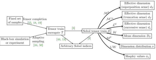
aggre-gations of up to exponential numbers of other indices. Figure 1 summarizes the state of the
art on TT-based SA and the algorithms here contributed, which build on the work from [3]
and thus reinforce all of the advantages of using the Sobol TT representation.
The rest of the paper is organized as follows. Section 2 reviews the main definitions and
concepts we use, including the analysis of variance (ANOVA) decomposition, the SI, and all
other sensitivity metrics considered. Section3outlines the mathematical tools that are
funda-mental for our algorithms: the tensor train (TT) decomposition as a framework for surrogate
modeling and the Sobol TT. In section 4 we contribute and construct explicitly several TT
tensors with 2N entries which behave as deterministic finite automata. In section 5 we show
how these automata can be combined with Sobol TTs to efficiently produce all sensitivity
met-rics listed in section2. Numerical results are presented in section 6, and concluding remarks
in section 7. Fixed set of samples Black-box simulation or experiment Tensor train surrogate\scrT
Arbitrary Sobol indices
Sobol tensor train\scrS
Effective dimension (superposition sense)dS Effective dimension (truncation sense)dT Effective dimension (successive sense)ds Mean dimensionDS
Dimension distribution\nu Shapley values\phi n
Tensor completion [55,18,19] Adaptive sampling [34,50] [3] [44,13] \scrM S [3] \scrM \leq n \scrL S \scrW \scrM S 1/\scrW
Figure 1. Previous work has established the TT model as a valuable tool for sensitivity analysis. Based on this, in this paper we explicitly construct several tensors (bold edges) that select and aggregate indices fromS
in convenient ways and produce a variety of advanced QoIs (rightmost boxes).
2. Sensitivity analysis: Definitions and metrics. We write multiarrays (tensors)
differ-ently depending on their dimension: italic scalars (e.g.,s), vectors with boldface italics (e.g.,
u), matrices with boldface capitals (e.g.,U), and higher-order tensors with calligraphic
capi-tals (e.g.,\scrT ). We point to their elements via NumPy-like notation, for example,\scrT [:,:k,:] are
the slices 0, . . . k - 1 of a 3D tensor along its second axis. The Kronecker and elementwise
products for matrices and tensors are written asU\otimes Vand\scrA \circ \scrB , respectively. Our accuracy
metric between a tensor \scrT and its approximation \scrT \widetilde (this includes vectors, matrices, etc.) is
always the relative error: \| \scrT - \scrT \| \widetilde /\| \scrT \| , where \| \cdot \| is the Frobenius norm (defined as the Euclidean norm of the tensor’s vectorization).
In this paper we often deal with tensors that have size 2N and use them to index tuples of
model variables. To access a position in a 2N TT tensor indexed by a tuple\alpha \alpha \alpha \subseteq \{ 1, . . . , N\}
we use subscripts: \scrT ααα \equiv \scrT [\alpha 1, . . . , \alpha N], where \alpha n = 1 if and only if n\in \alpha \alpha \alpha , and 0 otherwise.
For example, if\scrT is a 3D tensor of size 2\times 2\times 2, then\scrT 2,3 denotes the element\scrT [0,1,1]. We
write complements of tuples as - \alpha \alpha \alpha :=\{ 1, . . . , N\} \setminus \alpha \alpha \alpha .
2.1. ANOVA decomposition and Sobol indices. Let f : Ω \rightarrow \BbbR be an L2-integrable
function on a rectangle Ω = [0,1]N and F(x) = F1(x1)\cdot \cdot \cdot FN(xN) a separable probability
density function on Ω. The ANOVA decomposition, also known as the Sobol or Hoeffding
decomposition [23,52], splitsf into 2N terms, each of which depends on a different subset of
its input variables\{ 1, . . . , N\} :
(1) f(x) = \sum
ααα\subseteq \{ 1,...,N\}
fααα(x),
where eachfααα(x) only depends effectively onxααα and is built as
(2) \int Ω−ααα \left( f(x) - \sum βββ\subsetneq ααα fβββ(xβββ) \right) dF - ααα(x - ααα),
with f\emptyset (x) = f\emptyset = \BbbE [f] = \int
Ωf(x)dF(x). This defines a partition of the model’s statistical
variance as the sum of variances of each subfunction: Var[f] =\sum ααα\not =\emptyset Var[fααα].
The variance components, here denoted as Sααα, are the relative variance contributions of
each subfunction (except f\emptyset ), normalized by the total variance: Sααα := Var[fααα]/Var[f] for all
\alpha \alpha \alpha \not = \emptyset . They are nonnegative and sum up to 1. They are thus interpretable in terms of set
cardinalities and can be used to define a set algebra. The Sobol indices, or SI for short, are
specific aggregations and combinations of variance components. There are two main types,
namely, thetotal Sobol indices \scrS T (sometimes also known astotal effectsorfirst-order indices)
and theclosed Sobol indices \scrS C [38]:
(3) SαααT := \sum
β ββ\cap ααα\not =\emptyset
Sβββ, SαααC := \sum β β β\subseteq ααα Sβββ, which satisfy (4)
0\leq Sααα \leq SαααC \leq SαααT \leq 1,
SαααT = 1 - S - Cααα and SαααC = 1 - S - Tααα, \sum n Sn\leq 1\leq \sum n SnT.
2.2. Effective dimension. More advanced sensitivity metrics take into account the size
of the variable tuple\alpha \alpha \alpha . One example is the effective dimension, which has been defined in at
least three ways:
\bullet Superposition sense [8]:
dS:= arg min
k
\left\{
k\bigm| \bigm| \bigm| \sum
ααα\bigm| \bigm| | ααα| \leq k
Sααα\geq 1 - \epsilon
\right\} .
\bullet Truncation sense [8]:
dT := arg min
k
\Bigl\{
k\bigm| \bigm| \bigm| S\{ C1...k\} \geq 1 - \epsilon \Bigr\} .
\bullet Successive sense [29]:
ds:= arg min
k
\left\{
k\bigm| \bigm| \bigm| \sum
ααα\bigm| \bigm| len(ααα)\leq k
Sααα \geq 1 - \epsilon
\right\} .
In the above equation, len(\alpha \alpha \alpha ) := arg maxn\{ n \in \alpha \alpha \alpha \} - arg minn\{ n \in \alpha \alpha \alpha \} + 1 and \epsilon is a
small tolerance for unexplained effects (say, 5%). The superposition sense dS measures the
minimal order of interactions needed to capture most of the model variability. In other words,
it means that the model f is roughly a sum of dS-dimensional subfunctions; interactions
involving higher numbers of variables may be safely discarded. On the other hand, dT is the
number of leading variables needed to capture a 1 - \epsilon fraction of the variance. If we allow
reordering the variables, dT is the minimal integer such that there exists some tuple\alpha \alpha \alpha with
| \alpha \alpha \alpha | =dT such that SαααC \geq 1 - \epsilon . Last, ds is informative when all variables have an inherent
ordering, for example, in a time series; it means that the model consists of subfunctions that
depend on neighboring variables only.
2.3. Mean dimension. The mean dimension in the superposition sense [37] is the
ex-pected value of| \alpha \alpha \alpha | if one were to select\alpha \alpha \alpha with probability proportional to its variance:
(5) DS:=
\sum
α αα
Sααα\cdot | \alpha \alpha \alpha | .
With 3 variables, for example, DS = S1+\cdot \cdot \cdot + 2\cdot S1,2+\cdot \cdot \cdot + 3\cdot S1,2,3. This metric is
a noninteger number, unlike the effective dimension, and measures the average complexity or
dimensionality of a model. A result by Liu and Owen [30] states that the mean dimension
equals the sum of all first-order total SI: DS =\sum Nn=1STn.
2.4. Dimension distribution. Denoted as\nu , it was defined by Owen [37] as the probability
mass function of the random variable | \alpha \alpha \alpha | if one were to select\alpha \alpha \alpha as described before. It is a
discrete variable over the domain \{ 1, . . . , N\} , and each value 1\leq n\leq N has probability
(6) \nu (n) = \sum
α αα\bigm| \bigm| | ααα| =n
Sααα.
Its expected value is the mean dimension DS. Also, knowing the dimension distribution
allows a direct computation of the effective dimension in the superposition sense: if we write ¯
\nu := CDF(\nu ), then dS =\lceil \nu ¯ - 1(1 - \epsilon )\rceil .
2.5. Shapley values. They originated in game theory [51] to determine the just
retribu-tions that each individual player 1, . . . , N should receive from a set of potential coalitional
tasks: (7) \phi n:= \sum α α α\subseteq - \{ n\}
| \alpha \alpha \alpha | !(N - | \alpha \alpha \alpha | - 1)!
N! \cdot (Cααα\cup \{ n\} - Cααα).
Here Cααα represents the productivity or goodness of each coalition \alpha \alpha \alpha . Recently, Shapley
values have been reinterpreted as variance contributions in the context of SA, whereby a
connection with the SI was established [39]: If the productivity of each subset of variables\alpha \alpha \alpha is
taken to beCααα :=SαααC, then thenth Shapley value can be computed with the simpler formula
(8) \phi n=
\sum
ααα| n\in ααα
Sααα | \alpha \alpha \alpha | .
For example, \phi 1 = S1+S1,2/2 +S1,3/2 +S1,2,3/3. This interpretation has been further
investigated in various settings [53,25,40] and found to be a good compromise between the
more granular closed indices SC and the coarser total indices ST: it holds that S
n =SnC \leq
\phi n\leq SnT for all n= 1, . . . , N. It has been extended for the case of dependent input variables
as well. The Shapley values \phi also have the desirable property that their sum equals 1 [39],
unlike, for example, the total effects. 3. Tensor train decomposition.
3.1. Fundamentals. The tensor train (TT) model is a tensor decomposition proposed by
Oseledets [32] that is also known as alinear tensor network in other communities [21,10]. The
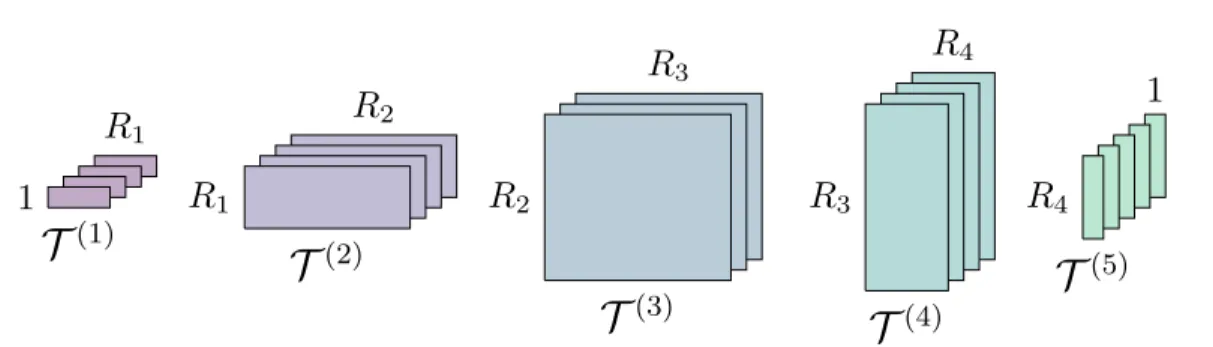
format assigns each physical dimension to one 3D core tensor (see Figure 2). To decompose
a model f into a tensor \scrT of size I1 \times \cdot \cdot \cdot \times IN, we first discretize each axis of the domain
Ω = Ω1\times \cdot \cdot \cdot \times ΩN so that f(x)\approx \scrT [i] with 0\leq in< In forn= 1, . . . , N. Elementwise, each
entry of\scrT is a product of matrices:
\scrT [i] =\scrT (1)[0, i1,:]\cdot \scrT (2)[:, i2,:]\cdot . . .\cdot \scrT (N - 1)[:, iN - 1,:]\cdot \scrT (N)[:, iN,0]
=
R - 1
\sum
r=0
\scrT (1)[0, i1, r1]\scrT (2)[r1, i2, r2]. . .\scrT (N - 1)[rN - 2, iN - 1, rN - 1]\scrT (N)[rN - 1, iN,0].
Every core \scrT (n) is thus a collection of matrices that are stacked along its second
dimen-sion (corresponding to the slices in Figure 2). The matrix sizes R1, . . . , RN - 1 are known
as TT ranks and capture the complexity of the compressed tensor. We sometimes write
\scrT = [[\scrT (1), . . . ,\scrT (N)]] to denote a TT decomposition in terms of its cores.
Let us write I := max\{ I1, . . . , IN\} and R := max\{ R1, . . . , RN - 1\} . The storage cost of a
TT tensor is O(N IR2), i.e., depends only linearly on the number of variables N. There is of
course no free lunch: the upper bounds forRare high, namely, R=IN/2 andO(IN) elements
are required to represent a tensor of sizeIN in the TT formatexactly in the worst case. This
happens when the (N/2)thTT unfolding matrix [32] (which has size IN/2\times IN/2 when N is
even) has full rank. Fortunately, in many applications this large matrix has many small (or
zero) singular values, and much lower values for R achieve sufficiently small error levels. See
also the discussion below.
R
1\scrT
(1)1
R
2\scrT
(2)R
1R
3\scrT
(3)R
2R
4\scrT
(4)R
31
\scrT
(5)R
4Figure 2. A5D tensor train approximating a tensor of spatial sizes4×4×3×4×5. Graphically, these sizes are the number of core slices (matrices) along the depth dimension, while the TT ranks(1, R1, R2, R3, R4,1) are distributed horizontally and vertically as matrix sizes. The ranks are usually larger around the central dimensions.
3.2. Black-box sampling for TT surrogate modeling. The TT format is a powerful gen-eralization of the matrix low-rank representation that can compactly encode the multidimen-sional structure of a wide family of functions and models. It has thus become a successful tool for high-dimensional interpolation and integration in physics and chemistry, and even in low
dimensions via the so-calledtensorization process [35] (which introduces artificial dimensions
in a vector via reshaping operations).
Given a black-box routine that can be evaluated on demand, one can often build an accurate TT representation of it via an adaptive sampling scheme over a structured set of
samples, for example, cross-approximation [34]. This is the method we use in this paper
to build all considered models and, although an in-depth discussion would be beyond the scope of this paper, we give here an introduction. Cross-approximation is best understood
as a generalization of the pseudoskeleton decomposition for matrices, which approximates a
matrix in terms of a number R of its columns and rows. The main challenge here is how to
select a good set of samples that is economic and yet spans the original matrix’s vector space
as accurately as possible. It was proven [16] that the best approximation is given by those
columns and rows whose intersection has maximal determinant in modulus, and an alternating
row/column selection heuristic was proposed that works well in practice [56]. For higher-order
tensors, columns and rows generalize tofibers, i.e., samples acquired by fixing all parameters
except one, which is moved throughout its full range. With cross-approximation these fibers
are chosen as columns and rows of various matricizations of the original tensor, which they
approximate by means of the pseudoskeleton decomposition. The more fibers are sampled, the larger TT cores one can construct, and the more accurate the approximation will be.
The numbers of TT ranksR1, . . . , RN - 1needed to achieve a good approximation (i.e., with
low relative error) are unknown a priori. Adaptive algorithms estimate them by starting with small cores that are progressively expanded as new fibers are sampled. The process is stopped
when the approximation is accurate enough, namely, when the relative error \| ˆx - x\| /\| x\|
between the new samples x and the current model’s estimation xˆ is below a user-defined
threshold. Thus, each sampling batch acts as a validation set plus stopping criterion. All in all,
for every dimensionn,O(RnInRn+1) samples are taken to fit a TT core of sizeRn\times In\times Rn+1.
The ranks often vary from core to core; for example, suppose that a modelf is separable with
respect to (w.r.t.) two groups of variables, f(x) = g(x1, . . . , xk)\cdot h(xk+1, . . . , xN). Then it
holds thatRk= 1, and good sampling heuristics will realize this after casting very few fibers
for that rank. Cross-approximation needsO(N IR2) samples overall to produce a compressed
tensor of O(N IR2) coefficients, so the number of function evaluations is proportional to the
number of degrees of freedom in the fitted model. The asymptotic complexity is O(N IR3)
operations (since, among other things, linear systems of size up toR\times R need to be solved),
so tensors with ranks up toR\approx 100 are usually tractable on a regular workstation in a matter
of seconds. This rank budget covers a large class of models, since low-rank structure is quite
frequent in practice [17]. A number of variants have been proposed to structure the adaptive
sampling plan [34,50,49, 7]. We make use of analternating minimal energy strategy [14] to
handle the rank selection, as is readily provided in the ttpy toolbox [36].
On top of surrogate modeling [57, 2, 17], the TT model has been used for sensitivity
analysis as well [13, 44, 59, 7, 3]. For a more in-depth review of TT model building
tech-niques from either fixed sets of samples or black-box settings, we also refer the reader to the
surveys [20,54].
3.3. Sobol tensor trains. The Sobol tensor train was recently introduced [3] as a
com-pressed TT tensor that can be extracted from anyN-variable TT surrogate model and
approx-imately represents its full set of 2N - 1 variance components and SI. Denoted by\scrS , the index
for any tuple\alpha \alpha \alpha is approximated by the corresponding tensor entrySααα\approx \scrS ααα =\scrS [\alpha 1, . . . , \alpha N].
Since \scrS is in the TT format, this entry is decompressed as a product of matrices:
(9) \scrS (1)[:, \alpha 1,:]\cdot . . .\cdot \scrS (N)[:, \alpha N,:].
The Sobol TT contains a 0 at the corner: \scrS \emptyset =\scrS [0, . . . ,0] = 0. It has size 2N (i.e., each
\alpha n can only take values in \{ 0,1\} ), and therefore each core has just 2 slices, as illustrated in
Figure 3for a 7D indexing example.
\scrS
(1)\scrS
(2)\scrS
(3)\scrS
(4)\scrS
(5)\scrS
(6)
\scrS
(7)Figure 3.A7-variable model yields a Sobol TTSof size27[3]. As an example, multiplying the7highlighted slices yields the elementS[0,0,0,1,0,0,1] =S4,7≈S4,7.
Throughout this paper we compute a TT surrogate to approximate each model studied
and extract its Sobol TT via the method described in [3]. The Sobol TT is, to our advantage,
a highly compact representation for the complete set of indices. Furthermore, many aggrega-tion and manipulaaggrega-tion operaaggrega-tions can be performed in the TT compressed domain, including
linear combinations (in O(N IR2) operations), differentiation/integration (O(N IR2) again),
and elementwise functions (O(N IR3) operations).
4. Tensor train masks. The sensitivity metrics in section2 rely on selecting and
weight-ing various indices accordweight-ing to their tuple order | \alpha \alpha \alpha | . We observe that these orders can be
appropriately and compactly accounted for in the TT format, thanks to a connection between
tensor networks and finite automata [12,43]. Next we contribute the explicit construction of
a number of weighted tensor masks and automata, followed by their application for the direct
computation of advanced metrics as further detailed in section5. All proposed TT masks are
N-dimensional, i.e., useN cores, and have 2N entries.
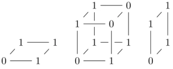
4.1. Hamming weight tensor. We define first the Hamming weight tensor \scrW , which
stores at each position\alpha \alpha \alpha \in \{ 0,1\} N the number of “1” elements in\alpha \alpha \alpha : \scrW
ααα := | \alpha \alpha \alpha | . Note that \scrW can be written as the sum of N separable terms. Each nth term has size 2N and adds 1
to each entry\alpha \alpha \alpha if and only if\alpha n= 1:
(10) \scrW = N \sum n=1 n - 1 terms \underbrace{} \underbrace{} \biggl( 1 1 \biggr)
\otimes \cdot \cdot \cdot \otimes
\biggl( 1 1 \biggr) \otimes \biggl( 0 1 \biggr) \otimes N - nterms \underbrace{} \underbrace{} \biggl( 1 1 \biggr)
\otimes \cdot \cdot \cdot \otimes
\biggl( 1 1 \biggr)
.
In the TT format, \scrW ’s rank is just 2. This is due to \scrW ααα =\alpha 1+\cdot \cdot \cdot +\alpha N being a purely
additive function. Such functions benefit from the following identity [33]:
(11)
N
\sum
n=1
\alpha n=\bigl( \alpha 1 1\bigr) \cdot \biggl(
1 0
\alpha 2 1 \biggr)
\cdot \cdot \cdot
\biggl( 1 0 \alpha N - 1 1 \biggr) \cdot \biggl( 1 \alpha N \biggr) .
Eachnth core consists of two slices: the first one is thenth matrix in (11), setting\alpha n= 0;
the second one is analogous but with\alpha n= 1. See Figure 4for an example illustration of this
construction for a 3-variable model.
1 1 0 1 1 0 1 0 1 1 0 1 1 1 1 0
Figure 4. The Hamming weight TT W for N = 3. At each position\alpha \alpha \alpha ∈ {0,1}N it records the bit sum
Wααα=|\alpha \alpha \alpha |. It is compressed withN cores (TT rank 2) using8N−8elements in total.
4.2. Hamming mask tensor. The N-dimensional Hamming mask tensor of type \leq n
contains a 1 at each entry\alpha \alpha \alpha if and only if | \alpha \alpha \alpha | \leq n, and a 0 otherwise. We denote it as \scrM \leq n.
It is equivalent to a deterministic finite automaton (DFA) that reads exactlyN symbols from
the input alphabet \{ ‘‘0”, “1”\} and has n+ 2 possible states\{ s0, s1, . . . , sn, R\} . There is an
accepting states0, . . . , snper each value of| \alpha \alpha \alpha | for which| \alpha \alpha \alpha | \leq n, and one extra rejecting state,
R, for any other value| \alpha \alpha \alpha | > n.
To construct a tensor equivalent to this automaton we need to mark one of the n+ 2
possible states as the active one at each processing step. We represent the active state with a
vector ofn+ 1 binary elements by usingdummy encoding, with the rejecting stateR encoded as the all-zeros vector. Each core updates the current state by multiplying the state vector generated in the previous step with the slice indexed by the corresponding input symbol. Thus, each slice encodes the state transition matrix for one of the input symbols (“0” or “1”).
Using these conventions, we manage to translate in a comprehensible manner our Hamming
mask automaton into a Hamming mask tensor (see also Figure5):
\bullet The state of the automaton after processing one input symbol can only be s0 if the
processed symbol was “0” (at [0,0,0]), ors1 if it was “1” (at [0,1,1]). Therefore, the
first core is all zeros in each slice except at those state positions.
\bullet The cores 2, . . . , N - 1 have as first slice (input “0”) an identity matrix so as to leave the state unchanged, while the second slice (input “1”) is the identity shifted to the right
since it is encoding the transition fromsj tosj+1by shifting any “1” in the input state
vector (bit at positionj) one position to the right (toj+ 1). An intuitive explanation
for these transition matrices is shown in the DFA state diagram of Figure 5, where
transitions labeled with the “0” input symbol always point to the current state and the ones labeled “1” point to the next state.
\bullet The last core collapses the state vector so that the result is “1” if and only if the
final state is one of the accepting states\{ s0, s1, . . . , sn\} after processing the last input
symbol, that is, ifnor fewer “1” bits were read. That means that for the last symbol
being a “0” any “1” in the state vector indicates an acceptable state\{ s0, . . . , sn\} , but
for the last symbol being a “1” the state vector cannot have a “1” in thesnth position.
Hence the first slice is all ones for checking the current state being within\{ s0, . . . , sn\} ,
and the second slice is all ones except for the last position to indicate the transition
from sn toR.
This pattern for building a Hamming mask tensor can be generalized to any length N
and any valuen by changing the number of cores toN and their rows and columns ton+ 1
accordingly, while always keeping 2 slices.
0 1 0 1 0 0 0 1 0 1 0 0 0 0 1 0 1 0 0 0 0 0 0 1 1 1 1 1 0 1 0 1 2 R 1 0 1 0 1 0
Figure 5. The Hamming mask TTM≤n for N = 3 andn = 2(left) and an equivalent DFA that reads
3symbols (right, “R” stands for the rejecting state). It contains a 1at every position\alpha \alpha \alpha ∈ {0,1}N such that
|\alpha \alpha \alpha |=n, and a 0everywhere else. It has TT rankn+ 1and uses2(n+ 1)2(N−2) + 4(n+ 1)elements.
4.3. Hamming state tensor. The last core of the mask tensor just described collapses
the state vector into one scalar (namely, 0 or 1) and depends onn. However, it is also useful
to output the Hamming weight using an explicit one-hot encoded result vector. We define the Hamming state tensor \scrM S, which maps every tuple\alpha \alpha \alpha to a vector ofN + 1 elements u, as
(12) ui=
\Biggl\{
1 ifi=| \alpha \alpha \alpha | ,
0 otherwise.
To build it we proceed similarly to \scrM \leq N and change the last core for a 3D one, namely,
the same as the central ones. So \scrM S has TT ranks 1, N + 1, . . . , N + 1, N + 1; i.e., it is
not a standard TT in the sense that its last rank is not 1. The Hamming state tensor needs
2(N+ 1)2(N - 1) + 2(N+ 1) elements to be stored.
4.4. Length tensors. The effective dimension in the successive sense motivates us to build
tensors that are sensitive to tuple length | \alpha \alpha \alpha | , i.e., the distance between the first and the last
variables present in the tuple. We define first thelength mask tensor \scrL \leq n, which filters tuples
of variables whose length exceeds a threshold (i.e., are too spread out). Elementwise,
(13) \scrL α\leq ααn:= \Biggl\{
1 if len(\alpha \alpha \alpha )\leq n,
0 otherwise.
We need again a state vector with n+ 1 elements to encode a state set with n+ 2 states
\{ s0, s1, . . . , sn, R\} using dummy encoding. As before, the rejecting state R is represented by
an all-zeros state vector. Any state transition will lead to R if a tuple length longer than
n is detected. An example of this tensor’s encoded automaton (n = 2, N = 3) is shown in
Figure 6:
\bullet The first core initializes the state vector in the same way as above in section 4.2.
\bullet The cores 2, . . . , N - 1 follow a regular pattern: the second slice is the identity shifted
to the right and therefore encodes the sj tosj+1 transition for any input state. The
first slice represents the transitions for the input symbol “0”, which in this case are more complex:
1. When the current state is s0 (a “1” in the first position of the state vector),
the output state should remain the same, and thus a “1” is placed at [0,0,0]
in the first row. This means that no input symbol “1” has been yet found, and thus the length counter remains at 0.
2. When the current state is s1, . . . , sn - 1 (a “1” in the second position of the
state vector in the example), the output state should be shifted to the next one, exactly in the same way as for an input “1”, and thus the same row as for the second slice.
3. When the current state is sn (a “1” in the third position of the state vector
in the example), the output state also remains sn. This encodes the case in
which the distance to the first input symbol “1” is already larger thann, and
therefore the condition will be violated as soon as an input symbol “1” appears. However, if the remaining input symbols are all “0” it would mean that the
actual distance to the last input symbol “1” was shorter than or equal to n,
and thus the final output would be “1”.
0 1 0 1 0 0 0 1 0 1 0 0 0 0 1 0 0 1 0 0 0 0 0 1 1 1 1 1 0 1 0 1 2 R 1 0 1 0 1 0
Figure 6. The length mask tensor L≤n for N = 3andn = 2(left) and an equivalent DFA that reads 3 symbols (right). It contains a 1at every position\alpha \alpha \alpha wherelen(\alpha \alpha \alpha )≤n, and 0otherwise. It uses the same ranks and number of elements asM≤n.
Table 1
Several tensors for the caseN= 5evaluated at three example tuples. Tuple\alpha \alpha \alpha Binary
form Wααα M ≤3 α α α MααSα L ≤3 α α α LSααα {5} [0,0,0,0,1] 1 1 [1,0,0,0,0] 1 [1,0,0,0,0] {1,5} [1,0,0,0,1] 2 1 [0,1,0,0,0] 0 [0,0,0,0,1] −{3}={1,2,4,5} [1,1,0,1,1] 4 0 [0,0,0,1,0] 0 [0,0,0,0,1]
\bullet The last core collapses the state vector to “1” if the final state belongs to the set of
accepted states in the same way as above in section4.2.
Based on this tensor and analogously to the Hamming state tensor (section4.3), we define
now thelength state tensor \scrL S, which maps every\alpha \alpha \alpha to a vector ofN+ 1 elements that stores
the value len(\alpha \alpha \alpha ) using one-hot encoding. It has the same storage complexity as \scrM S.
Table1shows a few examples of the values taken by the main tensors we have introduced
in this section.
5. Computing sensitivity metrics. In this section we show how the proposed tensors can be used to extract various SA metrics from any Sobol TT via efficient operations in the TT format (most importantly, tensor dot products and global optimization).
5.1. Mean dimension. Let us consider the formula for the mean dimensionDS:=\sum αααSααα\cdot | \alpha \alpha \alpha | , and let our Sobol TT \scrS contain all variance components S. We observe that, being a
weighted summation over all\alpha \alpha \alpha , the formula forDS equals the tensor dot product\langle \scrS ,\scrW \rangle . We
compute it by successively contracting the TT cores of \scrS and \scrW together (Algorithm1; see
also [32] and Algorithm 3 from [13]). Supposing that \scrS has a constant TT rank R =R1 =
\cdot \cdot \cdot =RN - 1, this has a total asymptotic cost ofO(N R2) operations.
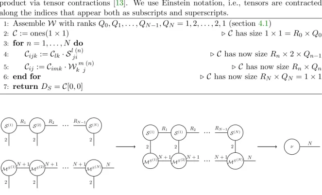
5.2. Dimension distribution. We can extract the complete dimension distribution
his-togram in one go via the Hamming state tensor, namely, by contracting\scrM S with\scrS along all
physical dimensions (Figure 7). The array we seek results from the remaining free edge; see
also Algorithm 2.
Algorithm 1. Given a Sobol TT \scrS , compute the mean dimension DS using fast TT dot
product via tensor contractions [13]. We use Einstein notation, i.e., tensors are contracted
along the indices that appear both as subscripts and superscripts.
1: Assemble\scrW with ranksQ0, Q1, . . . , QN - 1, QN = 1,2, . . . ,2,1 (section4.1)
2: \scrC := ones(1\times 1) \triangleleft \scrC has size 1\times 1 =R0\times Q0 3: forn= 1, . . . , N do
4: \scrC ijk:=\scrC lk\cdot \scrS lji(n) \triangleleft \scrC has now size Rn\times 2\times Qn - 1 5: \scrC ij :=\scrC imk\cdot \scrW k jm(n) \triangleleft \scrC has now sizeRn\times Qn 6: end for \triangleleft \scrC has now size RN \times QN = 1\times 1 7: return DS =\scrC [0,0] \scrS (1) \scrS (2) ... \scrS (N) \scrM S(1) \scrM S(2) ... \scrM S(N) \scrS (1) \scrS (1) ... \scrS (N) \scrM S(1) \scrM S(2) ... \scrM S(N) \nu R1 2 R2 2 RN−1 2 N+ 1 2 N+ 1 2 N+ 1 2 N R1 2 R2 2 RN−1 2 N+ 1 N+ 1 N+ 1 N N
Figure 7. We compute the dimension distribution vector\nu , which hasN elements, by contracting together the Sobol TT S (ranks1, R1, . . . , RN−1,1) with our proposed mask state tensor MS = [[MS(1), . . . ,MS(N)]] (ranks1, N+ 1, . . . , N+ 1,1) along their spatial and rank dimensions. All TT cores are collapsed together along Algorithm 1; this can be accomplished in O(N2R2) +O(N3R) operations. Only the N-sized edge from MS remains, and after the contraction it gathers all variance contributions according to their order, as expected.
Algorithm 2. Given a Sobol TT\scrS , compute the dimension distribution\nu .
1: Assemble\scrM S with ranks Q
0, Q1, . . . , QN - 1, QN = 1, N + 1, . . . , N + 1 (section5.1)
2: Contract \scrS with\scrM S as in Algorithm1
3: return \nu := resulting vector of N elements
5.3. Effective dimension (superposition sense). The variance due to order nand below is
(14) \sum
α α α\bigm| \bigm| | ααα| \leq n
\scrS ααα=
\sum
α α α
(\scrS \circ \scrM \leq n)ααα=\langle \scrS ,\scrM \leq n\rangle .
With (14) we can easily extract the superposed effective dimension: it is sufficient to
iteratively find the smallestk that yields a relative variance above the given threshold 1 - \epsilon ;
see also Algorithm 3.
Algorithm 3. Given a Sobol TT \scrS , compute its effective dimension (in the superposition
sense)dS w.r.t. threshold \epsilon .
1: Compute dimension distribution\nu as in Algorithm 2
2: \nu ¯:= cumulativeSum(\nu )
3: forn= 1, . . . , N do
4: if \nu ¯[n]\geq 1 - \epsilon then
5: return dS :=n 6: end if
7: end for
5.4. Effective dimension (truncation sense). The truncated effective dimension dT
de-pends on the ordering of variables [15]. However, the formula
(15) arg min
n
\Bigl\{
n\bigm| \bigm| max
α αα
\bigl\{
(\scrS \circ \scrM \leq n)ααα\bigr\} \geq 1 - \epsilon
\Bigr\}
gives us the truncated effective dimension w.r.t. the best possible ordering\alpha \alpha \alpha of variables. The
ncan be found iteratively (Algorithm 4). Note that the best (largest variance) order-ntuple
is given by finding the maximum of a 2N tensor. Although this is an NP-hard problem, we
exploit an existing global optimization heuristic based on cross-approximation [34, 13] that
only evaluates a subset of “promising” tensor entries. The method works well in practice and
is fast for tensors of moderate rank; see also [31].
Algorithm 4. Given a Sobol TT\scrS , compute its effective dimension (in the truncation sense)
dT w.r.t. threshold \epsilon and best possible ordering of variables.
1: Compute dimension distribution\nu as in Algorithm 2
2: forn= 1, . . . , N do
3: Assemble\scrM \leq n (section4.2)
4: v:= maxααα\{ \scrS \circ \scrM \leq n\} \triangleleft Elementwise product using cross-approximation [34], tensor
maximum found as in [13,31]
5: if v\geq 1 - \epsilon then
6: return ds:=n 7: end if
8: end for
5.5. Effective dimension (successive sense). The following dot product is the total
vari-ance contributed by all tuples whose length is nor less:
(16) 0\leq \langle \scrS ,\scrL \leq n\rangle \leq 1.
The effective dimension in the successive sense is therefore the smallestn (Algorithm5):
(17) ds= arg min
n
\bigl\{
n\bigm| \bigm| \langle \scrS ,\scrL \leq n\rangle \geq 1 - \epsilon \bigr\} .
Algorithm 5. Given a Sobol TT\scrS , compute its effective dimension (in the successive sense)
ds w.r.t. threshold\epsilon .
1: l:= the contraction between\scrS and \scrL S as in Algorithm2
2: ds := proceed as in Algorithm3but using linstead of\nu
3: return ds
5.6. Shapley values. The Shapley values can be interpreted as variance contributions in
an SA context and computed in terms of the SI [39]. They are considered a challenging QoI
from a computational point of view [39,40]: thenth value relies on 2N - 1 terms, each weighted
by a combinatorial number. Let the superscript\scrT C denote the closed version of a tensor \scrT ;
i.e., for each\alpha \alpha \alpha ,\scrT C α α
α is the sum of all \scrT βββ, where\beta \beta \beta \subseteq \alpha \alpha \alpha (recall (3)). We observe that, in tensor
form, the Shapley formula is equivalent to
(18) \phi n= \sum α α α| n\in ααα Sααα
| \alpha \alpha \alpha | = (\scrS \circ (1/\scrW )) C \{ n\} .
This represents the closed version of the weighted variance components, evaluated at
tuples \{ 1\} , . . . ,\{ N\} . Note that 1/\scrW is a so-calledHilbert tensor; such tensors are known to
have high rank but are extremely well compressible via low-rank expansions [34]. We have
confirmed this experimentally for this particular case in which the tensor has size 2N. For
N = 20, for example, compressing 1/\scrW using only R1 = \cdot \cdot \cdot = R19 = 7 ranks is enough
to achieve a relative error of 2.16\times 10 - 8 over the full set of 220 groundtruth values (we set
\scrW \emptyset :=\infty formally, i.e., 1/\scrW \emptyset = 0, to prevent division by 0). In Algorithm6 we show how to
compute all Shapley values\phi 1, . . . , \phi N using (18).
Algorithm 6. Given a Sobol TT\scrS , compute allN Shapley values.
1: Compute 1/\scrW \triangleleft Using cross-approximation. Can be precomputed
2: \scrS \widehat = [[S\widehat (1), . . . ,S\widehat (N)]] :=\scrS \circ (1/\scrW ) \triangleleft Denote its ranks as 1, Q1, . . . , QN - 1,1 3: forn= 1, . . . , N do \triangleleft Compute the closed tensor of a tensor [3] 4: \scrS \widehat (n)C := zeros(Qn - 1,2, Qn)
5: \scrS \widehat (n)C[:,0,:] :=\scrS \widehat (n)[:,0,:] \triangleleft The first slice stays the same 6: \scrS \widehat (n)C[:,1,:] :=\scrS \widehat (n)[:,0,:] +\scrS \widehat (n)[:,1,:] \triangleleft The second slice becomes the sum of both
slices 7: end for
8: \scrS \widehat C := [[\scrS \widehat (1)C, . . . ,\scrS \widehat (N)C]] 9: forn= 1, . . . , N do
10: \phi n:=\scrS \widehat \{ Cn\} =\scrS \widehat C[ n - 1 \underbrace{} \underbrace{} 0, . . . ,0,1, N - n \underbrace{} \underbrace{} 0, . . . ,0] 11: end for
12: return (\phi 1, . . . , \phi N)
6. Experimental results. We have tested our metric computation algorithms1 with three models of dimensionalities 10 and 20 on a desktop workstation (3.2GHz Intel i5). For each
model, a TT surrogate with 100 points per axis is built using adaptive cross-approximation [34,
50] as released in the Python library ttpy [36], from which we extract its Sobol TT using the
method from [3]. In all cases we compare all our resulting single-variable SI with the quasi–
Monte Carlo (QMC) algorithm by Saltelli et al. [46] implemented in the Sensitivity Analysis
Library for Python (SALib) [22], and our Shapley values with the state-of-the-art MC method
by Song, Nelson, and Staum [53]. We also assess the accuracy of the proposed algorithm for
the mean dimension DS by using the identity DS = \sum nSnT due to Liu and Owen [30]. We
report the number of function evaluations for each method.
6.1. Sobol “G” function. Our first model is synthetic and widely used for benchmarking purposes in the SA literature:
(19) f(x) := N \prod n=1 | 4xn - 2| +an 1 +an ,
withxn\sim \scrU (0,1) for alln. Coefficients an are customizable; we have chosen an:= (n - 2)/2
forn= 1, . . . , N as in [11]. This model is partly provided as a sanity check: sincef is separable (i.e., has TT rank 1), we can expect to obtain an exact TT interpolator over the discretized
grid. We tookN = 40 dimensions, i.e., the tensor grid has 10040 elements, and the resulting
Sobol TT encodes 240 \approx 1.1\times 1012 elements. We furthermore know the analytical values for
the SI from [27]: SC
n =Dn/D, STn =DTn/D for all n, where
(20) Dn= 1 3(1 +an)2 , DTn =Dn\cdot \prod i\not =n (1 +Di), D = - 1 + \prod n (1 +Dn).
Although separable, this model is very high-dimensional and therefore challenging for
MC-and QMC-based approaches. Adaptive cross-approximation here producedR1 =\cdot \cdot \cdot =R39=
1 as TT ranks, as is expected for a separable function. It took 123,400 samples in 2.18s and
achieved a relative error under 10 - 15. Since its Sobol TT cannot have a rank larger than
R2 = 1 [3], it is free of compression error (this applies to all product functions). Computing
the Sobol TT took 0.16s, whereas extracting all metrics took 9.69s. The most expensive
metric is the effective dimension in the truncation sensedT, since it requires several runs of a
global optimization algorithm (Algorithm4). Note also that since the ranks are all equal, all
slices along dimensions 1, . . . , N are visited the same number of times during sampling. For
this separable function, a minimum ofN \cdot I = 4,000 samples would be needed. However, the
practical algorithm does not know R a priori, so it does take extra samples and stops after
realizing that the error does not improve for R >1.
For comparison we run methods [46] (QMC for SI) and [53] (MC for Shapley values) with
5\times 106 and 40\times 106 samples, respectively. Note that the QMC method uses an extension of the Sobol sequence that does not require a power of two as the number of samples. Numerical
1Our algorithms are provided within the Python package athttps://github.com/rballester/ttrecipes (the
code for all models is available in the folderexamples/sensitivity analysis/).
Table 2
Sobol “G” function: effective and mean dimensions using our method. The mean dimension is compared with the analytical value, which is available for this model, and an estimation using the sum of total effects [30]
computed from QMC.
Dimension metric Value
Effective dimension (\epsilon = 0.05)
Superpositionsense (dS) 3 (98.1% variance) Truncationsense (dT) [X1 · · · X23 ] 23 (97.1% variance)
Successivesense (ds) 15 (95.2% variance)
Mean dimension (Ds) Exact 1.603 Ours 1.603 \sum nS T n (QMC [46]) 1.596 Table 3
Sobol “G” function: Shapley values and Sobol indices for the first and last 5variables.
Shapley value Closed Sobol index Total Sobol index
Ours MC [53] Ours Exact QMC [46] Ours Exact QMC [46]
X1 0.5036 0.5042 0.3322 0.3322 0.3324 0.7138 0.7138 0.7076 X2 0.1835 0.1750 0.0831 0.0830 0.0826 0.3122 0.3123 0.3144 X3 0.0898 0.0866 0.0369 0.0369 0.0373 0.1611 0.1612 0.1607 X4 0.0524 0.0499 0.0208 0.0208 0.0218 0.0961 0.0961 0.0963 X5 0.0341 0.0375 0.0133 0.0133 0.0131 0.0632 0.0632 0.0625 · · · · X36 0.0007 0.0024 0.0003 0.0003 0.0003 0.0013 0.0013 0.0013 X37 0.0006 0.0051 0.0002 0.0002 0.0002 0.0012 0.0012 0.0012 X38 0.0006 -0.0070 0.0002 0.0002 0.0002 0.0012 0.0012 0.0011 X39 0.0006 -0.0017 0.0002 0.0002 0.0002 0.0011 0.0011 0.0011 X40 0.0006 -0.0017 0.0002 0.0002 0.0003 0.0010 0.0010 0.0010
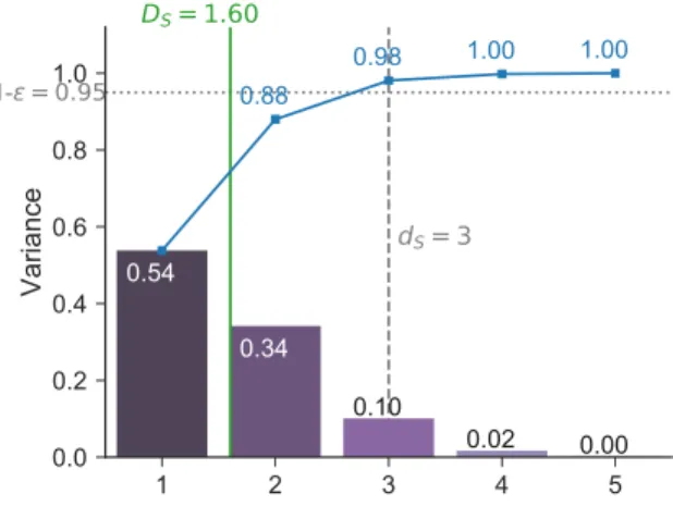
results are reported in Table 2 (effective and mean dimensions), Table 3 (Sobol/Shapley
indices), and Figure8 (dimension distribution). We always use the threshold\epsilon = 0.05 for the
effective dimensions; i.e., the proportion of variance preserved must be at least 95% (in Table2
we list the percentage achieved in each case). Note that the SI coincide with the groundtruth
by more than three decimal digits; specifically, the mean absolute error was 3.2\times 10 - 6 for the
Sn and 5.7\times 10 - 6 for the SnT. Note also that the QMC [46] only provides single-variable SI,
whereas the Sobol TT gives indices for interactions of all possible orders (only the first order is shown).
6.2. Simulated decay chain. The second example simulates a radioactive decay chain
that concatenates Poisson processes for 11 chemical species. It is a linear Jackson network;
i.e., each species (except the last one) can decay into the next species in the chain. In the beginning the material belongs entirely to the first species. We model 10 parameters,
namely, the decay rates \lambda n of the 10 first species. The simulation result fT(\lambda 1, . . . , \lambda 10) is
the amount of stable material (last node in the chain) measured after a certain time span
1 2 3 4 5 0.0 0.2 0.4 0.6 0.8 1.0 Variance 0.88 0.98 1.00 1.00 0.54 0.34 0.10 0.02 0.00 DS= 1.60 1- = 0.95 dS= 3
Figure 8. Sobol “G” function: dimension distribution (truncated after order 5), mean dimensionDS, and effective dimension in the superposition sensedS for\epsilon = 0.05.
T. To evaluate each sample offT we simulate the chain by discretizing the spanT into time
steps of one day. Each \lambda n is constant throughout all time steps and represents the fraction
of each material that decays every day. They are independent and uniformly distributed in
the interval [0.00063281,0.00756736], which corresponds to half-lives from 3 years down to 3
months.
The resulting effective and mean dimension metrics for a time span of T = 2 years are
reported in Table 4, and the Sobol and Shapley sensitivity indices in Table 5. The
cross-approximation sampling stage used 134,400 function evaluations (8.69s) and stopped after
achieving a relative error of 1.5\times 10 - 7. All TT ranks equal 6, so again the sampling plan
is evenly distributed among all slices. Building the Sobol TT took 0.06s, and extracting all
metrics took 0.76s. Methods [53] and [46] were run with 1.4\times 107 and 600,000 samples,
respectively. These were the minimal numbers such that their suggested confidence intervals
(one standard error for [46], two for [53]) were on average 10% of their estimated indices.
Note that our results converge unanimously to S1 = \cdot \cdot \cdot = S10, S1T = \cdot \cdot \cdot = S10T , and \phi 1 =
\cdot \cdot \cdot = \phi 10 = 1/10. This follows from the fact that the model is symmetric. We verified
experimentally that this equality still holds when we decreaseI orR, although results start to
deviate for small enough values of these hyperparameters. From this we learn that although restricting the sampling budget affects the final metric accuracy, cross-approximation stays robust at reflecting the symmetry of the model sampled.
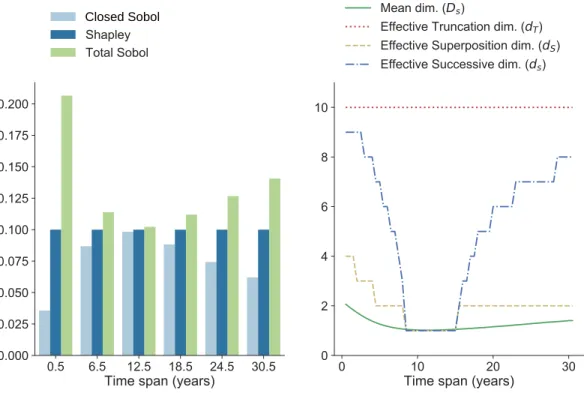
We have also studied the sensitivity behavior when varying the simulated time span: 0.5\leq T \leq 30.5 years (see dimension distributions in Figure9). Figure10depicts the evolution of the Shapley values, the SI, and the dimension metrics within the same range. Note how
the average interaction order is higher for extreme values ofT and lower in the center (\approx 1 at
around 12 years). This behavior hints that, for very short or long time spans, several decay rates need to have specific values to affect the output of the function. In the former case, for example, no amount of the final species is detected unless many decay rates are fast enough.
On the other hand, after a very long time spanT, all materials have decayed completely unless
several rates are slow enough. The successive dimensionds(right chart in Figure10) strongly
Table 4
Decay chain: effective and mean dimensions (time span = 2years).
Dimension metric Value
Effective dimension (\epsilon = 0.05)
Superpositionsense (dS) 3 (95.9% variance) Truncationsense (dT) [\lambda 1 · · · \lambda 10 ] 10 (100.0% variance) Successivesense (ds) 9 (97.8% variance)
Mean dimension (Ds) Ours 1.728 \sum nS T n (QMC [46]) 1.722 Table 5
Decay chain: Shapley values and Sobol indices (time span = 2years).
Variable Shapley value Sobol index Total Sobol index
Ours MC [53] Ours QMC [46] Ours QMC [46]
\lambda 1 0.100 0.096 0.049 0.049 0.173 0.171 \lambda 2 0.100 0.099 0.049 0.052 0.173 0.171 \lambda 3 0.100 0.093 0.049 0.050 0.173 0.170 \lambda 4 0.100 0.102 0.049 0.049 0.173 0.171 \lambda 5 0.100 0.100 0.049 0.048 0.173 0.167 \lambda 6 0.100 0.099 0.049 0.050 0.173 0.184 \lambda 7 0.100 0.111 0.049 0.051 0.173 0.171 \lambda 8 0.100 0.109 0.049 0.051 0.173 0.170 \lambda 9 0.100 0.096 0.049 0.048 0.173 0.172 \lambda 10 0.100 0.097 0.049 0.050 0.173 0.176
reflects this behavior as well: the metric is highly sensitive to such high-order consecutive interactions and is therefore useful for these kinds of time-series models.
Finally, this example illustrates how the Shapley values\phi nare able to recognize the equal
importance of all variables and act as the best overall summary of their influence. This is
consistent with Owen [39], their original proponent in the context of SA.
6.3. Fire-spread model. Last we model the rate of fire spread in the Mediterranean
shrublands according to 10 variables that are fed into Rothermel’s equations [45]. Both [48]
and [53] have analyzed this model from the SA perspective. We compare our results with
the latter work for the case of independently (but nonuniformly) distributed parameters. We
use the updated equations as in [53], which incorporates the modifications by Albini [1] and
Catchpole and Catchpole [9], with the marginal distributions shown in Table 6.
Cross-approximation took 4.72\times 106 samples in 8.28s and achieved a relative error of
5.3\times 10 - 5 with TT ranks (11,17,17,7,43,16,16,11,6). The sixth core has size 43\times 100\times 16 and is the largest we encountered so far; this means that relatively many sample fibers were
needed along variablemd. Building the Sobol TT took 0.28s, and extracting all metrics took
0.52s. Method [53] was run with 4.6\times 107 samples (just as in the original paper), while we
again ran method [46] so as to attain a 10% confidence interval (6.96\times 106 samples). Results
are reported in Table7(effective and mean dimensions) and Table 8(Shapley values and SI)
0.0
0.5
1.0
Variance
0.70 0.90 0.98 1.00 0.36 0.35 0.20 0.07 0.02 DS= 2.07Time span = 0.5 years
0.99 1.00 1.00 1.00 0.87
0.12 0.01 0.00 0.00
DS= 1.14
Time span = 6.5 years
0.99 1.00 1.00 1.00 0.98
0.01 0.01 0.00 -0.00
DS= 1.02
Time span = 12.5 years
1
2
3
4
5
0.0
0.5
1.0
Variance
1.00 1.00 1.00 1.00 0.88 0.12 0.00 0.00 0.00 DS= 1.12Time span = 18.5 years
1
2
3
4
5
0.99 1.00 1.00 1.00 0.74
0.25 0.01 0.00 0.00
DS= 1.27
Time span = 24.5 years
1
2
3
4
5
0.97 1.00 1.00 1.00 0.62 0.35 0.02 0.00 0.00 DS= 1.41Time span = 30.5 years
Figure 9.Decay chain: mean dimension and dimension distribution (truncated after order5) for 6different time spans0.5≤T ≤30. Very short and very long time spans result in higher-order interactions.
Closed Sobol
Figure 10. Decay chain: all metrics as a function of the time span. In the left plot, each index is averaged across all variables. Note how the closed and total SI follow an inverse relationship with one another and meet at aboutT = 12years, whereas the Shapley values are constant.
Table 6
Fire spread: parameter description and marginal distributions [53].
Variable Description Distribution
\delta Fuel depth (cm) LogN(2.19,0.517)∩[5,∞)
\sigma Fuel particle area-to-volume ratio (1/cm) LogN(3.31,0.294)
h Fuel particle low heat content (Kcal/kg) LogN(8.48,0.063)
\rho p Oven-dry particle density (D.W.g/cm3) LogN(−0.592,0.219)
ml Moisture content of the live fuel (H2O g/D.W.g) N(1.18,0.377)∩[0,∞)
md Moisture content of the dead fuel (H2O g/D.W.g) N(0.19,0.047)
ST Fuel particle total mineral content (MIN.g/D.W.g) N(0.049,0.011)∩[0,∞)
U Wind speed at midflame height (km/h) 6.9·LogN(1.0174,0.5569)
tan\phi Slope N(0.38,0.186)∩[0,∞)
P Dead to total fuel loading ratio LogN(−2.19,0.64)∩(−∞,1]
Table 7
Fire spread: effective and mean dimensions.
Dimension metric Value
Effective dimension (\epsilon = 0.05)
Superpositionsense (dS) 3 (97.6% variance)
Truncation sense (dT) [\delta ,\sigma ,ml,md,U,P ] 6 (96.1% variance)
Successivesense (ds) 8 (96.5% variance)
Mean dimension (Ds) Ours 1.650 \sum nS T n (QMC [46]) 1.714 Table 8
Fire spread: Shapley values and Sobol indices.
Variable Shapley value Closed Sobol index Total Sobol index
Ours MC [53] Ours QMC [46] Ours QMC [46]
\delta 0.203 0.217 0.106 0.106 0.331 0.348 \sigma 0.125 0.132 0.048 0.048 0.235 0.228 h 0.003 -0.020 0.001 0.001 0.005 0.006 \rho p 0.012 0.013 0.004 0.005 0.023 0.023 ml 0.231 0.231 0.142 0.143 0.346 0.364 md 0.165 0.183 0.095 0.097 0.259 0.262 ST 0.002 -0.006 0.001 0.001 0.005 0.004 U 0.202 0.210 0.090 0.093 0.354 0.387 tan\phi 0.004 -0.014 0.002 0.002 0.006 0.006 P 0.053 0.054 0.029 0.029 0.086 0.086
as well as in Figure 11 (dimension distribution). The analytical metrics for this model are
unknown, but our results are in all cases within the other two methods’ intervals of confidence. 7. Discussion and conclusions. The Sobol indices have long been in the spotlight of the variance-based sensitivity analysis and uncertainty quantification communities. In recent years, several other sensitivity metrics that capitalize on these building blocks and are
1 2 3 4 5 0.0 0.2 0.4 0.6 0.8 1.0 Variance 0.86 0.98 1.00 1.00 0.52 0.34 0.12 0.02 0.00 DS= 1.65 1- = 0.95 dS= 3
Figure 11. Fire spread: dimension distribution (truncated after order 5).
binatorial in nature have increased in popularity. State-of-the-art algorithms and sampling schemes that estimate these advanced metrics often require rather large numbers of samples, i.e., in the order of millions of function evaluations. Therefore, modern methods are grow-ingly dependent on fast analytical or surrogate models in order to keep overall computation times low. We found that, in many cases, similar or lower sampling budgets are actually suf-ficient to build highly accurate TT surrogates. Once such a tensor representation is available, its advantages become evident: a wide range of operations can be computed expeditiously in the compressed domain, including differentiation, integration, optimization, elementwise dot products and functions, and in particular fast evaluation of many sensitivity metrics, as proposed in this paper.
All proposed TT automata are error-free and highly compact, since they can compress
masks of size 2N using onlyO(N3) (and often fewer) elements. Given a high-quality surrogate,
they allow us to extract metrics that are close to their analytical values by several decimal digits of precision. Constructing the tensor masks is a fast procedure: one first “compiles” an algorithm (automaton) into a compressed tensor by organizing sparse arrays (TT cores) in a certain configuration that is determined by the automaton’s type and dimensionality. The algorithm is then “executed” by computing its tensor dot product with the target Sobol TT. This dot product is an iterative algorithm on its own, namely, a sequence of tensor contractions that boil down to simple matrix-matrix products and array reshaping operations.
To summarize, we have contributed algorithms for advanced variance-based sensitivity analysis that leverage tensor decompositions heavily, in particular the TT model. Such de-compositions can represent exponential numbers of indices and QoIs in an extremely compact manner. Throughout our paper we exploited three crucial tools. First, the Sobol TT is able to gather all variance components. While most surrogate-based SA approaches use a metamodel as a departure point for metric computation, we go one step further and work with a data structure that already contains all elementary indices of interest. Second, the automaton-inspired TT tensors contributed here are in charge of selecting and weighing index tuples as needed, and they all have a moderate rank. Last, tensor-tensor contractions (i.e., dot prod-ucts) in the TT format have a polynomial cost w.r.t. number of dimensions and, combined
with the previous elements, can produce sophisticated QoIs in a matter of a few sequential steps. Other auxiliary (but still important) tools include adaptive cross-approximation, which is useful for building TT surrogates and auxiliary tensors, and global optimization in the compressed domain.
Limitations and future work. Our main limitation is the critical assumption that the model of interest admits a low- or moderate-rank TT representation. It is known that various classes of tensors may be better compressed via alternative tensor networks, and we are actually confident that the proposed methods and automata are adaptable to other network topologies. Other techniques that remain promising to combine and improve TT compression
include dimension reordering [6] and active subspace transformations [4].
On another note, the particular case remains of how to extract reliable sensitivity metrics when limited by modest sampling budgets, e.g., of a few hundreds or thousands of samples. Using an intermediate surrogate is often the method of choice in these cases, as well as for the
other state-of-the-art methods [41]. On the TT side, one may either use cross-approximation
on the intermediate model or build directly the tensor from a limited set of samples using low-rank tensor completion techniques; see, e.g., the positive recent results by Gorodetsky
and Jakeman [17]. Research on TT completion usually strives for a generalization error as
low as possible, as estimated, for example, by cross-validation strategies. Here we deal with derived quantities of interest whose computation does not add additional error, but that will be affected nonetheless by the surrogate’s generalization error. Future research efforts will be directed toward better characterizing how inaccuracy due to a small sampling budget can have an impact on derived sensitivity metrics.
Acknowledgment. The authors wish to thank Eunhye Song for providing code for the
fire-spread model [53].
REFERENCES
[1] F. A. Albini, Estimating Wildfire Behavior and Effects, tech. report, U.S. Department of Agriculture, Intermountain Forest and Range Experiment Station, 1976.
[2] R. Ballester-Ripoll, E. G. Paredes, and R. Pajarola,A surrogate visualization model using the tensor train format, in Proceedings of the SIGGRAPH ASIA 2016 Symposium on Visualization, 2016, pp. 13:1–13:8.
[3] R. Ballester-Ripoll, E. G. Paredes, and R. Pajarola,Sobol Tensor Trains for Global Sensitivity Analysis, preprint,https://arxiv.org/abs/1712.00233, 2017
[4] V. Baranov and I. V. Oseledets,Fitting high-dimensional potential energy surface using active sub-space and tensor train (AS+TT) method, J. Chem. Phys., 143 (2015), 17417.
[5] M. Bianchetti, S. Kucherenko, and S. Scoleri, Pricing and Risk Management with High-Dimensional Quasi Monte Carlo and Global Sensitivity Analysis, preprint, https://arxiv.org/abs/ 1504.02896, 2015.
[6] D. Bigoni and A. Engsig-Karup,Uncertainty Quantification with Applications to Engineering
Prob-lems, Ph.D. thesis, Technical University of Denmark, 2015.
[7] D. Bigoni, A. P. Engsig-Karup, and Y. M. Marzouk,Spectral tensor-train decomposition, SIAM J.
Sci. Comput., 38 (2016), pp. A2405–A2439,https://doi.org/10.1137/15M1036919.
[8] R. E. Caflisch, W. J. Morokoff, and A. B. Owen, Valuation of Mortgage Backed Securities Us-ing Brownian Bridges to Reduce Effective Dimension, CAM report, Department of Mathematics, University of California, Los Angeles, 1997.
![Figure 3. A 7-variable model yields a Sobol TT S of size 2 7 [3]. As an example, multiplying the 7 highlighted slices yields the element S[0, 0, 0, 1, 0, 0, 1] = S 4,7 ≈ S 4,7 .](https://thumb-us.123doks.com/thumbv2/123dok_us/11081299.2994637/9.918.154.729.699.829/figure-variable-yields-sobol-example-multiplying-highlighted-element.webp)