Towards a Computational Analysis of Probabilistic Argumentation Frameworks

Technological University Dublin Technological University Dublin

ARROW@TU Dublin

ARROW@TU Dublin

Articles School of Computing

2014

Towards a Computational Analysis of Probabilistic Argumentation

Towards a Computational Analysis of Probabilistic Argumentation

Frameworks

Frameworks

Technological University Dublin, [email protected]

Follow this and additional works at: https://arrow.tudublin.ie/scschcomart

Part of the Artificial Intelligence and Robotics Commons, and the Theory and Algorithms Commons Recommended Citation

Recommended Citation

Dondio, P. (2014) Towards a Computational Analysis of Probabilistic Argumentation Frameworks. Cybernetics and systems [to appear in 2014] doi:10.1080/01969722.2014.894854

This Article is brought to you for free and open access by the School of Computing at ARROW@TU Dublin. It has been accepted for inclusion in Articles by an authorized administrator of ARROW@TU Dublin. For more

information, please contact

[email protected], [email protected], [email protected].

This work is licensed under a Creative Commons Attribution-Noncommercial-Share Alike 3.0 License

Towards a Computational Analysis of Probabilistic

Argumentation Frameworks

PIERPAOLO DONDIO1

1

School of Computing,

Dublin Institute of Technology, Kevin Street 2, Dublin, Ireland

In this paper we analyze probabilistic argumentation frameworks (PAFs), defined as an extension of Dung abstract argumentation frameworks in which each argument is asserted with a probability . The debate around PAFs has so far centered on their theoretical definition and basic properties. This work contributes to their computational analysis by proposing a first recursive algorithm to compute the probability of acceptance of each argument under grounded and preferred semantics, and by studying the behavior of PAFs with respect to reinstatement, cycles and changes in argument structure. The computational tools proposed may provide strategic information for agents selecting the next step in an open argumentation process and they represent a contribution in the debate about gradualism in abstract argumentation.

KEYWORDS: Argumentation Theory, Probabilistic Reasoning, Abstract Argumentation, Grounded and Preferred Semantics

INTRODUCTION

An abstract argumentation framework is a direct graph where nodes represent arguments and arrows represent the attack relation. Abstract argumentation frameworks [13, 9] were introduced by Dung [2] to analyze properties of defeasible arguments, i.e. arguments whose validity can be disputed by other conflicting arguments.

Various semantics have been defined to identify the set of acceptable arguments. In this work we deal with grounded and preferred semantics and we follow the labeling approach proposed by Caminada [7], where a semantics assigns to each argument a label in, out or undec, meaning that the argument is considered consistently acceptable, non-acceptable or undecided (i.e. one abstains from an opinion).

In Dung’s original work, arguments are treated as abstract entities that are either fully asserted or not asserted at all, and there are no degrees related to either arguments or relations of attacks. Abstract argumentation is often too strict and coarse to support a decision making process. The situation is described by Dunne et al. [11], who notice how the solution provided by abstract argumentation “is often an empty set or several sets with nothing to distinguish between them”. Abstract argumentation has proven to be efficient in keeping the logical consistency of conflicting evidence, but there are limited extensions that can be practically deployed to handle gradualism. Some approaches have tried to marry probability calculus and argumentation semantics, defining probabilistic argumentation frameworks. In a an

argumentation semantics is used to identify under which conditions a set of arguments are acceptable, while probability calculus quantifies how likely those conditions are.

The study of PAFs is still at an embryonic stage. Debate has centered on their correct theoretical definition and some basic properties derived from abstract argumentation. There is no computational algorithm proposed beside the brute force approach, and no study over their behavior w.r.t. to reinstatement or sensitivity to changes in the argumentation structure.

Taking stock of previous research in the area, we first modify some formal definitions of concepts. However, these definitions are anchored in previous works and do not represent the major contribution of the paper. Our key contribution is represented by a set of new computational tools developed for analyzing : we describe the first recursive algorithm to compute the probability of acceptance of each argument and we study the behavior of w.r.t. to reinstatement, cycles and changes in the arguments structure. Our work represents a contribution to the introduction of gradualism in argumentation.

The paper is organized as follows: in the first two sections we recall the pre-requisites of abstract argumentation and PAFs; we describe the very first algorithm to compute the acceptance probabilities of the arguments. We then describe the behavior of w.r.t. to reinstatement and cycles, we analyze the behavior of in relation to changes and we propose an application of , before discussing related works.

BACKGROUND DEFINITIONS

Definition 1. (Abstract Argumentation Framework) Let be the universe of all possible

arguments. An argumentation framework is a pair ( , ) where is a finite subset of and ⊆ × is the attack relation.

Let us consider AF = (Ar , R ) and Args ⊆ Ar.

Definition 2. (conflict-free). is conflict-free iff ∄ , ∈ |

Definition 3. (defense). defends an argument ⊆ iff

∀ !ℎ #ℎ # , ∃ ! !ℎ #ℎ # ! . The set of arguments defended by is denoted ( ).

Definition 4. (indirect attack/defense) Let , ∈ r and the graph % defined by ( , ). Then (1) indirectly attacks if there is an odd-length path from to in the attack graph % and (2) indirectly defends if there is an even-length path from to in %.

Two arguments and are rebuttals iff ( , ) ∧ ( , ).

Labeling. A semantics identifies a set of arguments that can survive the conflicts

encoded by the attack relation . In this work we follow the labeling approach of Caminada et al. [7], where a semantics assigns to each argument a label in, out or undec.

Definition 5. (labeling/conflict free). Let = ( , ) be an argumentation framework. A labeling is a total function ' ∶ → {+ , , #, -.!}. We write in(L) for { |'( ) = + }, out(L) for { |'( ) = , #}, and undec(L) for { |'( ) = -.!}. A labeling is conflict-free if no in-labeled argument attacks an in-labeled argument.

Definition 6. (complete labeling, from Definition 5 in [7]). Let ( , ) be an argumentation framework. A complete labeling is a labeling that for every holds that:1. if is labeled + then all attackers of are labeled , #; 2. if all attackers of are labeled , #

then is labeled + ; 3. if is labeled , # then has an attacker labeled + ; 4. if has an attacker labeled + then is labeled , #

Theorem 1. (from [7]) Let L be a labeling of argumentation framework ( , . It holds that L is a complete labeling i

ff

Theorem 2. (from theorem 6 and 7 in [7]) Let , be an argumentation framework. ' is the grounded labeling iff L is a complete labeling where undec(L) is maximal (w.r.t. set inclusion) among all complete labelings of . L is the preferred labeling iff L is a complete labeling where + ' , , # ' are maximal.

In figure 1 two argumentation graphs are depicted. Grounded semantics assigns the status of undec to all the arguments of , since it represents the complete labeling with the maximal undec-set, while in 1 , according to theorem 1, there is only one complete labeling (that is thus grounded and preferred), where argument is in (no attackers), is out and ! results in in. Note how reinstates !. Regarding (A), there are two complete labelings where in(L) is maximal w.r.t. to set inclusion: one with + '₂ * /, , # '₂ * , !/, -.! '2 ∅ and the other with + '4 * , !/ and , # '4 * / and -.! '4 ∅.

Figure 1. Two Argumentation Graphs (A) and (B)

PROBABILISTIC ARGUMENTATION FRAMEWORKS

In this section we present earlier work in probabilistic argumentation frameworks that we progress. We start from the concept of and its meaning. In the first work by Li [4], a probability measure is attached to each argument and attack relation of an abstract argumentation framework. Li et al. define these probabilities as the “likelihood of existence of an argument or attack relation” on the argumentation graph [4]. In [6], Hunter progresses the conceptual notion of . He admits that “what is meant by the probability of an argument holding is an open question”. He proposes a justification prospective similar to [4], where the probability indicates the degree to which the argument belongs (or is believed to belong) to the graph. Yet he also proposes an alternative view, referred to as the premises perspective on argument probability of being true. In this approach, the probability of each argument is based on the degree to which its premises are true, or are believed to be true. Our stance is closer to Hunter’s second view. Since an argument’s premises are affected by probabilistic uncertainty, we are left with an argument whose claim is affected by the same uncertainty, meaning that the claim holds with likelihood 5, and does not hold with likelihood 1 7 5.

We report the definition proposed by Li [4] used as baseline reference for this paper: A probabilistic argumentation framework PrAF is a tuple , ₈ , 9, _: where , 9 is an abstract argumentation framework, ₈ ∶ → 0 ∶ 1< and _: ∶ 9 → 0 ∶ 1<.

Key elements of Li et al.’s definition are the use of a probability for both arguments and attacks and the assumption of argument and attack independence (hence ₈ and _: are scalar

numbers). Central to this is the way argument probability of acceptance is computed. The probabilistic nature of arguments, common to Li et al., Hunter and our research, implies that given an argumentation framework of elements, 2 different scenarios are possible, each of them obtained by assuming each argument or attack relation to exist or not. Li et al. call these scenarios induced argumentation frameworks, each corresponding to a subgraph of the starting argumentation framework. Each induced argumentation framework has a probability of existing attached to it, computed by applying the product rule using ₈ and _:, and each induced framework behaves as an abstract Dung-style framework.

Thus, given a semantics (although only grounded semantics is analysed in [4]), Li et al. define the probability of acceptance of an extension as the sum of the probabilities of all the induced frameworks where the chosen semantics produce that extension. This computation, that requires computing the chosen semantic in all the subgraphs of the original argumentation framework, is referred to by Hunter as the constellation approach. Hunter [6] extends some of Li et al.’s definitions and investigates the situations where arguments might not be independent and the probability is given as a joint probability distribution.

Our Definition and its Differences from Previous Works

Definition 7. (PAF). A probabilistic argumentation framework PAF is a couple , )

where = ( , ) is an abstract argumentation framework with a finite set of arguments and an attack relation on × ; and is a joint probability distribution over .

Our contribution to the formal definition of is minor, and our definition is an extension of the previous work of Li et al. and Hunter. However, in the next section we will introduce new definitions of argument acceptability used in our computational analysis and based on the above definition, and it is thus important to make these modifications clear and explicit. Referring to Li et al.’s definition as a baseline, our differs in the following respects: probabilities are only attached to arguments and induced frameworks are only identified by subsets of nodes, the probability P is a joint probability rather than a scalar function. Moreover, as described in the next section, we define acceptability at argument level rather than at extension level, we also introduce the probability of an argument to be labeled out or undec, we extend the definitions of the probability of argument acceptance by adding the credulous and skeptical acceptance of preferred semantics.

We end this section by clarifying some concepts of our definition that are not discussed by Li et al. and Hunter, but that are useful to better understanding our computational analysis. In the definition of a PAF, given a generic argument , ( ) is the probability that holds on its own, in isolation, before the dialectical process starts. It is the likelihood that the probabilistic premises of the argument are true, and thus the argument claim can be used in the argumentation process. Our aim is to compute the probabilities >?( ), @AB( ), _A( ) that a generic argument will be labeled in, out or undec under the chosen semantics. Algorithm 1 proposes a brute force approach to computing _>? ( @AB, _A are analogous).

The difference between ( ) and >?( ) is crucial. If ( ) is the probability of argument ’s claim to hold in isolation, before the argumentation process combines arguments,

>?( ) is the probability of being labeled in by the chosen semantics. >?( ) entails the

effect of the argumentation process on , i.e. the fact that ’s conclusion might be invalidated by other arguments. Argument could have a high probability of holding in isolation, but be

completely invalidated in argumentation. It may be that : Joe got full marks in his math test, so he is good at math, but it might be also known that : Joe copied the test. Thus

1, but since attacks , then _>? 0 (the conclusion does not hold anymore) . Algorithm 1 - Brute force approach for computing C_DE

for each sub-graph % of ,

use to compute the probability % of % for each argument in %

assign a label F to in % using the chosen semantics

if F + add % to _>? Formalizing Scenarios and their Probabilities

Given an argumentation framework , with | | , and the graph % identified by and , we consider the set G of all the subgraphs of %. We define specific sets of subgraphs, i.e. elements of 2I. Given ∈ r, we define:

* ∈ G | ∈ / ; ̅ * ∈ G | ∉ / (1)

that are respectively the set of subgraphs where argument is present and the set of subgraphs where is not present (note how we use ̅ for the complementary set L).

We define a scenario as the argumentation framework identified by the subgraph and the restriction of to . A scenario models the situation in which some arguments are assumed to hold and are present in the argumentation process and some arguments are assumed not to hold and are discarded from the dialectical process.

In general, we can express a set of subgraphs (and corresponding scenarios) combining some of the sets ₂, . . , ,MMM, . . , MMMM₂ . with the connectives *∪,∩/. We write 1 to denote ∩ 1 and P 1 for ∪ 1. For instance, in figure 1 the single subgraph/scenario with only and ! present is denoted with ̅1Q, while the expression 1 denotes a set of two subgraphs/scenarios where arguments and are present and ! can be either present or not.

We call clause R a finite intersection (or conjunction) of sets _S , U_T. We consider expressions of sets of scenarios in their disjunctive normal form, i.e. as a finite disjunction of clauses R₂P R₄P. . PR_V.

It is possible to compute the probability of each subgraph/scenario starting from the probability . If * ₂, . . , /, a single scenario/subgraph is a clause of length modeling a generic situation in which _W probabilistic arguments are assumed to hold while the other

7 X are not. The probability _Y of this generic scenario is the joint probability:

Y 2∧ 4∧ … ∧ W∧MMMMMM ∧ … ∧ MMM[\2 ) (2)

The probability of a set of scenarios _YY is the sum of the probabilities of each scenario in the set. Thus, regarding the set of scenarios , by marginalization on argument :

YY ∑Y∈8 Y and YY ̅ 1 7 (3)

Since every set of scenarios can be expressed by the conjunction of expressions containing only the sets _S , U_T, using the above equation the probability of any set of subgraphs can be

Labeling Scenarios and Acceptance

Given a scenario ∈ a (a being the set of all the scenarios), the labeling of follows the rules of the chosen semantics. We define a scenario labeling ℒ as a total function over the Cartesian product of arguments in and scenarios in a, thus ℒ: Ar × S → {+ , , #, -.!}. When labeling a scenario, we follow this choice: an argument is labeled out in all the scenarios where does not hold (i.e. it is out because it is assumed not to hold on its own) or when it holds but it is labeled out by the semantics, representing the effect on of other arguments.

Regarding grounded semantics there is only one labeling per scenario , that we call

ℒe_{( ). In the case of preferred labeling there could be more than one valid labeling per}

scenario. Each preferred labeling for scenario is referred to as ℒ_Sfg( ) and the set of the preferred labelings of a scenario as hfg( ) = {ℒ₂fg( ), . . , ℒfg( )}. We call + (ℒi( )),

, #(ℒi_{( )), -.!(ℒ}i_{( )) the sets of argument labeled in, out, undec in ℒ}i_{( ), with 5}

denoting the semantics used (either or ). In order to study how an argument behaves across scenarios in a, we define the following set of scenarios. For grounded semantics:

>?e = { ∈ a: ∈ + (ℒe, )} ; @ABe = { ∈ a: ∈ , #(ℒe, )} A

e _{= { ∈ a: ∈ -.!(ℒ}e_{, )}}

which represent all the scenarios where argument is labeled in, out or undec. Regarding preferred semantics, since there could be more than one labeling for each scenario , we define two extreme sets corresponding to skeptical and credulous attitudes. The credulous set is identified by requiring argument to be labeled in at least in one of the valid preferred labelings for . Hence we define:

>? fg\_{= k ∈ a: l∃ ℒ}fg_{( ) ∈ h}fg_{( ) ∶ ∈ + (ℒ}fg_{, )mn} @AB fg\ = k ∈ a: l∃ ℒfg_{( ) ∈ h}fg_{( ) ∶ ∈ , #(ℒ}fg_{, )mn} A fg\_{= k ∈ a: l∃ ℒ}fg_{( ) ∈ h}fg_{( ) ∶ ∈ -.!(ℒ}fg_{, )mn}

While the skeptical sets are:

>? fgo ₌ >? fg_{∖ l} @AB fg _⋃ A fg_{m ;} @AB fgo ₌ @AB fg _{∖ (} >? fg_⋃ A fg₎ ; _Afgo= _Afg∖ ( _@ABfg ⋃ _>?fg) (4) representing scenarios where argument has the same label in all the preferred labeling of a scenario. It is _>?fgo⊆ _>?fg\, _@ABfgo ⊆ _@ABfg\, _Afgo ⊆ _Afg\ and the two sets of scenarios identify an upper and lower probability level. We add a last useful notation. We write _rst for all the scenarios where holds and it results labeled out. Note that _@AB = ̅ + _rst.

Definition 8. We define the probabilities of acceptance (5), of rejection (6) and

undecided probability (7) of argument for grounded and preferred semantics as follows:

8e = ( >?e ), 8\ = ( >?fg\), 8o = ( >?fgo) (5) 8e

MMMM = ( _@ABe ₎

,MMMM = (₈\ _@ABfg\),MMMM = (₈o _@ABfgo) (6)

8e = ( Ae), 8o = ( Afgo), 8\ = ( fg\A ) (7)

Example 1 Let us consider the graph of figure 1 (A), and let us study the properties of

argument . There are 3 arguments, thus 2u 8 scenarios. Let us presume 1 Q 0.8 and , , ! are statistically independent. Let us start computing _>?e . Argument is

labeled in in all the scenarios where it holds and does not hold (and ! becomes irrelevant). Using our notation 1M (i.e. the set of subgraphs {* /, { , !}}. It is undec when all the arguments are present, i.e. the single scenario _Ae = 1Q (i.e. {{ , , !}}) and it is labeled out when it is assumed not to hold or when is in and ! is out, i.e. _@ABe = ̅ + 1Q̅ (set

{∅, { }, {!}, { , }, { , !}}). By inserting numerical values we have:

8e = 0.16, 8e = 0.512, MMMM = 0.3288e .

Regarding preferred semantics, we can verify that:

>? fg\ = 1M + 1Q , l >?fg\m ≡ 8\ = 0.672 >? fgo_{= 1M, l} >? fgo_{m ≡} 8o = 0.16 A fg\ = Afgo = ∅ @AB fg\ _{= ̅ + 1,} @AB fg\ _≡ 8\ MMMM = 0.84 @AB fgo _{= ̅ + 1Q̅,} @AB fgo _≡ 8o MMMM = 0.328.

COMPUTING }_DE: A RECURSIVE ALGORITHM

This section presents an algorithm to compute _>?, _@AB under grounded semantics. Given a starting argument and a label F ∈ {+ , , #}, we need to find the set of subgraphs where argument is legally labeled in. The idea is to traverse the transpose graph (a graph with reversed arrows) from down to its attackers, propagating the constraints of the grounded labeling. While traversing the graph, the various paths correspond to a set of subgraphs. The constraints needed are listed in definition 5 and theorem 1. If argument – attacked by n arguments 5 – is required to be labeled + , we impose the set _>? to be:

>? = ∩ l~_2@AB∩ ~_4@AB∩ … ∩ ~ _@ABm condition (1)

i.e. argument can be labeled in in the subgraphs where: 1. is present in the subgraph (i.e. the set and

2. all the attacking arguments 5_S are labeled , # (sets ~_S@AB . If is required to be labeled , #, the set of subgraphs is:

@AB = ̅ ∪ ∩ l~_2>?∪ ~_4>?∪ … ∪ ~ _>?m condition (2)

i.e. is labeled , # in all the subgraphs where it is not present or at least one of the attackers is labeled + . Thus we recursively traverse the graph, finding the subgraphs that are compatible with the starting label of . The sets ~ _@AB, ~ _>? are found when terminal nodes are reached. When a terminal node 5_B is reached the following conditions are applied:

1. if 5_B is required to be + then ~_B>?= ~_B

2. if node 5_B is required to be , # then ~_B@AB = ~MMMM_B

The way the algorithm treats cycles guarantees that only grounded complete labelings are identified. If a cycle is detected, the recursion path terminates, returning an empty set that also has the effect of discarding all the sets of subgraphs linked with a logical •9 (by condition 1) to the cyclic path. We present the pseudo-code of the algorithm, while Table 1 describes the steps for computing _>? in the graph of figure 2 right.

Algorithm 2 - The Recursive FindSet(A,L,P) Algorithm

A is a node, L a label (IN or OUT), P is the list of parent nodes, Cset holds the partial result of the computation of conditions (1) and (2).

FindSet(A,L,P): if A in P:

return empty_set // Cycle found

if L = IN: if A terminal:

return a // Terminal condition for IN Label else:

add A to P

for each child C of A

Cset = Cset AND FindSet(C,OUT,P)

return (a AND Cset) // condition 1

if L = OUT: if A terminal:

return NOT(a) // Terminal condition for OUT Label else

add A to P

for each child C of A

Cset = Cset OR FindSet(C,IN,P)

return (NOT(a) OR (a AND Cset)) //condition 2

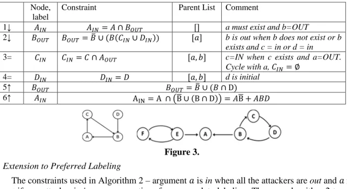
Table 1. Recursively applying Algorithm 2 on the graph of figure 3 left. Node,

label

Constraint Parent List Comment

1↓ _{>? >?}= ∩ 1_@AB €< a must exist and b=OUT

2↓ 1_@AB 1_@AB 1M ∪ 1 Q_>?∪ 9_>? € < b is out when b does not exist or b exists and c = in or d = in

3= Q_>? Q_>? Q ∩ _@AB € , < c=IN when c exists and a=OUT. Cycle with a, Q_>? ∅ 4= 9_>? 9_>? 9 € , < d is initial 5↑ 1_@AB 1_@AB 1M ∪ 1 ∩ D 6↑ _{>? A‚ƒ A ∩ lBU ∪ B ∩ D m BU P 19} Figure 3.

Extension to Preferred Labeling

The constraints used in Algorithm 2 – argument is in when all the attackers are out and is out if one attacker is in – are properties of any complete labeling. The way algorithm 2 treats cycles – it always assigns the undec label to their arguments – guarantees that we collect only grounded complete labeling. Since a preferred labeling is complete, the extension of algorithm 2 to the case of preferred semantics requires changing only the way cycles are treated. The following lemma is useful in always assigning an argument labeled in in a complete labeling to the computation of _>?fg\.

Lemma 1. If is labeled in (or out) in a complete labeling of a scenario, then the

scenario can be assigned to _>?fg\ (or _@ABfg\).

Proof. If is labeled in in a complete labeling Q of a scenario , either Q is the preferred one maximizing + Q, w.r.t. to set inclusion, or there is another Q’ with + Q, ⊂ + Q‡, . Since ∈ + Q, , then ∈ + Q‡, and scenario contributes to fg\_>? .

We return to the treatment of cycles. When a cycle is detected, the labeling of an even-length cycle is consistent since the argument that is visited twice and identifies the cycle is required to have the same label. However, an odd-length cycle creates an inconsistent undec labeling not contributing to _>?fg\ or _@ABfg\. Thus we assign a clause (i.e. set of scenarios) to

>? fg\

when a consistent cycle is found, while we reject the scenario otherwise. Note how the skeptical sets _>?fgo and _@ABfgo can be derived once the credulous sets are computed using equations 4. In traversing the graph, we thus need to remember the label required for an argument to check if the cycle can be consistently labeled. It is important to bear in mind that

rst (small letter for the label) identifies the set of scenarios where argument exists and it is

labeled out (note that _@AB = ̅ + _rst). Let us consider the graph depicted in figure 3 left. This contains both odd and even length cycles. Table 2 shows the steps in computing _>?\ .

Table 2. Computing _>?fg\ of figure 3 left

1 _>?= 1_@ABˆ_@AB 2a 1_@AB= 1M + 1_rst9_>? 2b ˆ_@AB= ˆM + ˆ_{rst >?} 3a _{1rst9>?= 1rst9Q@AB} 3b _{ˆrst >? = ˆrst ˆ@AB} 4a _{1rst9Q@AB= 1rst9Q̅ + 1rst9Q1>?} = 19Q̅ + ∅ + !, + #. # !‰!F. 4b _{ˆrst ˆ@AB= ˆ} !, + #. # !‰!F.: . - Š .5+ # , . = + , Š = , # 5a _{1@AB= 1M + 19Q̅} 5b _{ˆ@AB= ˆM + ˆ} 6 _>?\ = 1M + 19Q̅ ˆM + ˆ = 1MˆM + 1Mˆ + 19Q̅ˆM + 19Q̅ˆ

Note how the 3-length cycle creates an inconsistent situation 1_rst9Q1_>? (argument has to exist and be labeled in and out at the same time) while ˆ_rst ˆ_@AB can be labeled consistently (the cycle is consistent when argument . is required to exist and labeled out). We can verify that o_>? differs from _>?\ since it discards the even-length cycle ˆ , thus the path ˆ (and any path in an and condition with it) are not in _>?o .

Notable Examples: Accrual of Attacks

Let us consider the in figure 4 left. Argument is labeled in iff holds and both and

! are labeled out (satisfied only when and ! do not hold, since and ! are inital). Thus:

>?= 1QMMMM ; @AB = ̅ + 1 + 1MQ

which represents the accrual of a probabilistic network. Note how this differs from mainstream numerical argumentation approaches where no accrual occurs [9, 1] and the effect of n arguments can be equated with the effect of the argument with the maximum degree. In the probabilistic accrual every argument counts, to the extent given by their joint probability.

Figure 4. Accrual (left), Reinstatement (center) and a circle of arguments (right).

Notable Examples: Reinstatement

When an argument attacks , argument is in iff exists and does not hold, thus

>?= 1M, @AB ̅ P 1. The case of 3 isolated arguments (figure 4 center) is useful in

analyzing the reinstatement property. It is easy to verify this:

>? 1M P 1Q , @AB ̅ P 1Q̅

In the generic case of arguments, _>? we have:

>? 1MMM P 12 2141MMM P ⋯ ; u @AB ̅ P 121MMM P 14 2141u1MMM P ⋯Œ

The statistical independence of arguments makes evident some reinstatement properties. By using the fact that ~ 1 7 ~M the expression of _>? can be written as follows:

>? 7 2 P 2 4 7 ⋯

Note how _>? is the sum of the probabilities of all the paths terminating in . The paths terminating with a defender (odd length) are positive factors contributing to _>? and vice versa for the path ending with an attacker of . The reinstatement effect of attackers and defenders decreases with the length of the path, but all influence _>? .

We now compare the reinstatement of a to other argumentation approaches.

PAF. An argument is always reinstated but with a lower probability (note how it is fully reinstated only when ! 1). All the arguments on the chain contribute to the reinstatement with decreasing effect.

Dung’s Abstract AF. In an abstract argumentation framework, arguments in a chain are reinstated at full potential, since the chain is made up of both in arguments (defended by the initial argument) and out arguments (attacked by the initial argument).

Pollock [9]. The arguments presented in [9] have a degree of justification in •_Ž\. This degree is a subtractable cardinal quantity. Referring to figure 4 center, when an argument c of degree J_‘ attacks of degree J_’ then the new degree of after the attack is J_’‡ max J_’7 J‘, 0 and J–‡ max J‡’7 J–, 0 . Thus argument is fully reinstated when J‘ — J’, and not

reinstated (at all) if J_’‡ — J_– while in all other cases it is reinstated proportionally to J_’7 J_‘. Note how, unlike a , it is relative comparison of degrees that decides the reinstatement.

Cayrol and Lagasquie-Schiex's vs-defense. In [1], a strength is attached to attack relations. Argument is fully reinstated iff S_’‘ ˜ S_’–, otherwise it remains totally defeated. Thus it is the relative comparison of the strength of the attacks that defines reinstatement. We notice that, although attack from C to B is logically antecedent to that from B to A, it is neglected if S_‘’™ S_’–. Generally, apart from , the distance of an argument from the first node in the chain is not linked to its impact on and the strength of reinstatement is usually a relative comparison of strength, with the consequence that some attacks might be neglected.

In the case of arguments forming a cycle, let us consider the case of two arguments and rebutting each other. In a PAF with grounded semantics we have:

>? e

= 1 U , _@ABe = U , _Ae = 1

>? is unchanged compared to the case where attacks but not vice versa, while the not

null _A decreases _@AB. The counter attack from to does not improve _>? . This is the expected behavior of grounded semantics: an argument cannot reinstate itself but it needs a third external argument. In the case of grounded semantics, the skeptical set _>?\ neglects the attacker ( _>?\ = since fully reinstates itself; the skeptical set is equal to the grounded case ( _>?o = 1 U . It is also _Ao = _A\ = ∅ and _@AB\ = U + 1, _@ABo = U

SENSITIVITY TO CHANGES IN OR

The expression of _>? ( _@AB or _A) allows us to study a set of properties of argument in relation to the arguments in . An interesting set of properties is the study of the sensitivity of

>? to a change in the probability of an argument (for instance when new evidence on its

validity are found); or to the addition/removal of an argument to/from (here we limit to the situation of adding an argument attacking or rebutting an argument in ).

The interest is mainly due to its applications: an agent might want to understand the effect of extra evidence affecting an argument, or which are the arguments that have the maximum impact on _>? . In a legal dispute, a lawyer deciding on his/her its strategy might focus on which arguments he should challenge in court. We first define two useful measurements of change.

Definition 9. The partial differential gain of argument w.r.t. to argument is š›œ• ž š› Ÿ

The sign of the differential gain tells whether an argument should be attacked or defended in order to increase _>? , while its value quantifies the impact of the argument on .

Definition 10. We call argument a dialectical defender of iff š›œ• ž

š› Ÿ > 0, and is

a dialectical attacker of when š›œ• ž

š› Ÿ < 0

Let us now define a particular expression of _>?, that contains information about how the behaves in relation to changes.

Definition 11. Given an argument and an argument for which there is at least a

path from to , we call the normal form of _>? w.r.t. to the following expression of _>?:

>?= ~1 + 1M + Q, with ~ ∩ = ∅.

The term ~1 represents the set of scenarios contributing to _>? where argument is assumed to hold. 1M represents the set of scenarios contributing to _>? but requiring not to hold. Q is the set of scenarios contributing to _>? where the status of is irrelevant.

It can be proved that argument is always labeled in in the set ~1. If, ad absurdum, is labeled out in a scenario in ~1, then the same scenario where does not hold has the same labeling and it would also contribute to _>? and thus the status of would have been irrelevant and the scenario would have been part of the set Q and not ~1, contradicting the hypothesis. Hence we can rewrite the normal form as follows:

>?= ~1>?+ 1M + Q , with ~ ∩ = ∅.

Why is this form useful? The expression makes explicit the contribution of arg. to

>?.When = = ∅ , >? = Q and does not contribute to >? and thus >? . A change in

w.r.t. is null. If ~ = ∅ then _>? = 1M + Q. We can compute the dialectical gain w.r.t. argument . In the rest of this section, we use also for _^^ to simplify the notation (bearing in mind how the probability distribution _^^ defined over a set of scenarios is derived from the distribution defined over arguments, as shown in equation 3).

We compute the dialectical gain by first evaluating the difference in _>? when is increased by ∆ . Since = 1 − M , a change in of ∆ is a decrement of lMm by

∆ , and since 1M = ∧ 1M = |1M 1M = |1M lMm we write:

>? \∆Ÿ− >? = |1M l lMm − ∆ m − |1M lMm = − |1M ∆ < 0

The differential gain is:

¢ >?

¢ = lim∆Ÿ→Ž

>? \∆Ÿ− >?

∆ = − l ¥Mm < 0

meaning that incrementing will decrease the value of _>? , thus making a dialectical attacker of . In case of statistical independence we have š›œ• ž

š› Ÿ = − .

Similarly, if = ∅ then results a dialectical defender and the differential gain is

~| . We bear in mind that is constant in the computation while _>? varies. In the general case, when both ~ and are not empty, is a defender when ~| >

l ¥Mm and an attacker when ~| < l ¥Mm. Thus:

Proposition 1. Given the normal form of _>? w.r.t. b _>? = ~1_>?+ 1M + Q, the differential dialectical gain of w.r.t. to is:

¢ >?

¢ = ~| − l ¥Mm

In case of statistical independence of arguments it is: š›œ• ž

š› Ÿ = ~ −

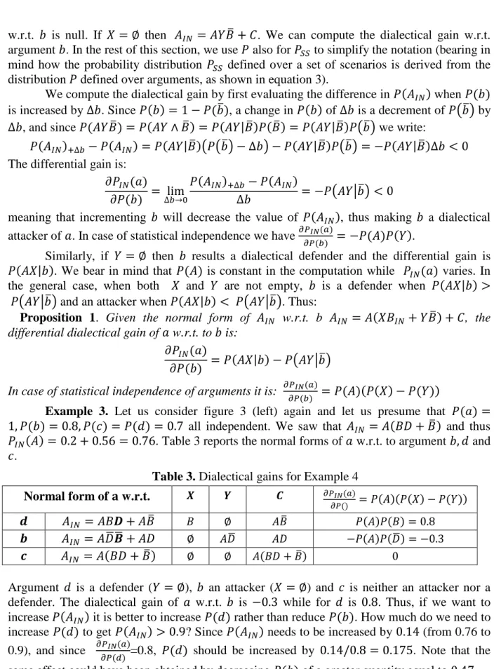
Example 3. Let us consider figure 3 (left) again and let us presume that =

1, = 0.8, ! = - = 0.7 all independent. We saw that _>?= 19 + 1M and thus

>? = 0.2 + 0.56 = 0.76. Table 3 reports the normal forms of w.r.t. to argument , - and

!.

Table 3. Dialectical gains for Example 4

Normal form of ¦ w.r.t. § ¨ © š›œ• ž

š› = ~ −

ª >?= 1« + 1M 1 ∅ 1M 1 = 0.8

¬ >? = 9U-U + 9 ∅ 9U 9 − 9U = −0.3

® >? = 19 + 1M ∅ ∅ 19 + 1M 0

Argument - is a defender ( = ∅), an attacker (~ = ∅) and ! is neither an attacker nor a defender. The dialectical gain of w.r.t. is −0.3 while for - is 0.8. Thus, if we want to increase _>? it is better to increase - rather than reduce . How much do we need to increase - to get _>? > 0.9? Since _>? needs to be increased by 0.14 (from 0.76 to 0.9), and since š›œ• ž

š› ° =0.8, - should be increased by 0.14/0.8 = 0.175. Note that the

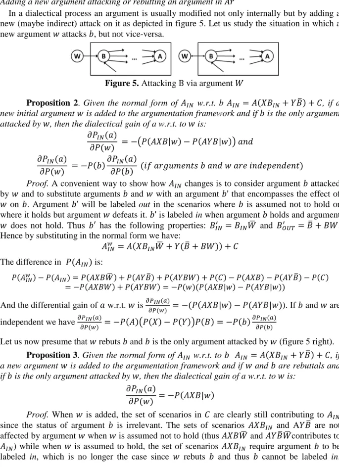
Adding a new argument attacking or rebutting an argument in

In a dialectical process an argument is usually modified not only internally but by adding a new (maybe indirect) attack on it as depicted in figure 5. Let us study the situation in which a new argument ² attacks , but not vice-versa.

Figure 5. Attacking B via argument ³

Proposition 2. Given the normal form of _>? w.r.t. b _>? = ~1_>?+ 1M + Q, if a new initial argument ² is added to the argumentation framework and if is the only argument attacked by ², then the dialectical gain of a w.r.t. to ² is:

¢ >? ¢ ² = −l ~1|² − 1|² m -¢ >? ¢ ² = − ¢ >? ¢ +Š ´. # - ² . + -. . -. #

Proof. A convenient way to show how _>? changes is to consider argument attacked by ² and to substitute arguments and ² with an argument ’ that encompasses the effect of ² on . Argument ’ will be labeled out in the scenarios where is assumed not to hold or where it holds but argument ² defeats it. ’ is labeled in when argument holds and argument ² does not hold. Thus ′ has the following properties: 1_>?‡ 1_>?³U and 1_@AB‡ 1M P 1³. Hence by substituting in the normal form we have:

>?

¶ _~1

>?³U P 1M P 1³ P Q

The difference in _>? is:

>? ¶ ₇

>? ~1³U P 1M P 1³ P Q 7 ~1 7 1M 7 Q

7 ~1³ P 1³ 7 ² ~1|² 7 1|²

And the differential gain of w.r.t. ² is š›œ• ž

š› ¶ 7 ~1|² 7 1|² ). If and ² are

independent we have š›œ• ž

š› ¶ 7 l ~ 7 m 1 7

š›_œ• ž š› Ÿ

Let us now presume that ² rebuts and is the only argument attacked by ² (figure 5 right).

Proposition 3. Given the normal form of _>? w.r.t. to _>? ~1_>?P 1M P Q, if a new argument ² is added to the argumentation framework and if ² and are rebuttals and if is the only argument attacked by ², then the dialectical gain of a w.r.t. to ² is:

¢ >?

¢ ² 7 ~1|²

Proof. When ² is added, the set of scenarios in Q are clearly still contributing to _>? since the status of argument is irrelevant. The sets of scenarios ~1_>? and A 1M are not affected by argument ² when ² is assumed not to hold (thus ~1³U and 1M³Ucontributes to

>?) while when ² is assumed to hold, the set of scenarios ~1>? require argument to be

Regarding the scenarios in 1M, they still contribute to _>? since is required not to hold and so ² is disconnected from and therefore irrelevant. Thus:

>? · _{= ³U ~1 + 1M + Q + ³ 1M + Q = ~1³U+ 1M + Q} >? · ₋ >? = ~1³U + 1M + Q − ~1 − 1M − Q = − ~1³ = − ² ~1|²)

And the differential gain of a w.r.t. ² is š›œ•(ž)

š›(¶) = − ( ~1|²). In the case of the statistical

independence of arguments, it is: š›_š›(¶)œ•(ž)= − ( ) (~) ( )

We note how the dialectical gains w.r.t. and ² have opposite sign, as expected. In the case of a rebuttal, proposition 3 states that the dialectical gain is always negative or null (when

~ = ∅), consequence of the fact that a rebuttal under grounded semantics does not defeat the attacked argument.

Example 4. We continue example 3, where we found that š›œ•(ž)

š›(°) =0.8 and

š›_œ•(ž) š›(Ÿ) = −0.3. Let us presume that we could attack argument - and we want again to bring ( >?) above 0.9. If we attack - we have no way to increase ( _>?), since the dialectical gain of w.r.t. - is positive. Let us consider argument . The normal form is 9U1M + 9 and the dialectical gain w.r.t. to is −0.3. If we attack with a new argument ², according to prop. 2, the dialectical gain is −0.3 ∗ − ( ) = 0.24. In order to increase _>? by 0.14, argument ² should at least have a strength of 0.14/0.24, about 0.583. If we rebut argument with ², since

~ = ∅ in the normal form w.r.t. , proposition 3 tells us that argument ² would have no effect. AN EXAMPLE OF APPLICATION: A LEGAL CASE

In order to make our applicable, we must provide a structure for arguments and attacks. We describe a single rule argument model adapted from [10], that keeps the discussion simple, but is adequate for illustration. Let us consider a set of atomic propositions = { ₂, . . , } and the propositional language ℒ closed under negation with atoms in and connectives {∧, ¬}. We define an argument as a defeasible inference rule of the kind: R → ¹ where R, ¹ ∈ ℒ. Defeasible means that a rule admits exceptions and it can be invalidated by other arguments. Note how our definition is limits argument to a single rule (adequate for our illustrative example), instead of including derivation trees composed by chain of rules as in [10].

If we call ℛ is the set of rules, we define a function of conflict U : ℒ → 2ℒ∪ 2ℛ, that allows us to define asymmetric conflicts among propositions and rules. If = M then when is asserted cannot be asserted, but not viceversa. It is = ¬MMMM and ¬ = M. If = ̅ and is a rule, this means that is an exception to rule , when is asserted is invalid. Note how this function models conflicts, but also preferences: = M could model the fact that is preferred to . Each argument has an associated probability equal to the probability R of its premises R (this means we know the joint probability of all the propositions used in the premises of the arguments, representing our available evidence used to build arguments). We define three forms of attack: rebuttals, undermining and undercutting. Given two arguments : R₈ → ¹₈ and 1: R_»→ ¹_», we say that rebuts 1 iff ¹₈ = ¹MMMM_» and ¹_» = ¹MMMM₈, undermines 1 iff

undercuts 1 iff ¹₈ = 1M, i.e. the conclusion ¹₈ invalidates the rule 1. An undercutting attack model the fact that defeasible rules (such as 1) might have exceptions (such as ¹₈). Note how a rebuttal is always a symmetric attack, an undermining could be (it is iff ¹₈ = RMMMM_» and

R» = ¹MMMM8), while an undercut is always defined as asymmetric (the exception defeats the rule

but not viceversa). Given a set of arguments of the kind R_S → ¹_S, we can represent them on a , , using as the probability of each argument R_S , and using rebuttals and undercutting attack to define the attack relation .

We present an application of to legal reasoning. Paul and John are on trial for the assassination of Sam. The following evidence is available. First it is known with certainty that John entered the room where the murder took place at 1 pm and left at 3 pm, while Paul entered at 3 pm and he was found by the police at 5 pm. A forensic test suggests that the probability that Sam died between 1 pm and 3 pm is 0.6 and between 3 pm and 5 pm is 0.4. The test used has an accuracy of 0.9. Thus we have the following arguments (in square brackets the probability of each premise):

¼½ 2: (John was in the room between 1 to 3 [1]) ∧ 4: (the medical test says that Sam died

between 1 and 3 [0.6] ) _{→ u}: (John shot Sam)

¼C Œ: (Paul was in the room between 3 and 5 [1]) ∧ ¾: (the test says that Sam died

between 3 and 5 [0.4]) _{→ ¿}: (Paul shot Sam)

ÀÁ Â: (The test is void [0.1]) → MMM ∧Ã MMMM› (Sam’s time of death cannot be estimated)

The probability of each argument is: _Ã 0.6, _› 0.4 and Ä_t 0.1. We also have l Ã∧ ›m 0, since Sam either died between 1 and 3 pm or between 3 and 5 pm. Argument

Ät undercuts (invalidates) both à and ›. Since à 0.6 — 0.5 — ›, John’s lawyer asks for

a fingerprint analysis of the murder weapon. The result is that with a probability of 0.7 the fingerprints are Paul’s. The lawyer thus proposes a new argument:

ÅC Æ: ( The test says that the fingerprints are Paul’s [0.7])→ ¿: (Paul shot Sam)

This argument rebuts _Ã (conclusions are conflicting, since it is clearly _u MMM_¿ and

¿ MMMu). In any case, further analysis by the police labs states that the weapon was tampered

with, and the test is only 50% reliable. The new argument (with a probability of 0.5): ÇÅ È: ( the test is void [0.5]) → MMM› (fingerprints are not valid evidence)

undercuts the validity of _›. Paul’s lawyer counter-attacks using the testimony of a credible witness who heard a shot at 2 pm, when only John was in the room. The witness is reputable with a probability of 0.8. Thus the following argument is built by the judge:

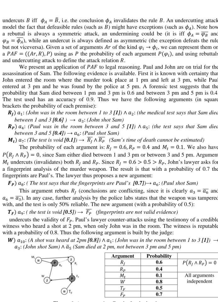
É 2Ž: (A shot was heard at 2pm [0.8]) ∧ 2: (John was in the room between 1 to 3 [1]) → u: (John shot Sam) ∧ M¾ (Sam died at 2 pm, not between 3 pm and 5 pm)

Figure 6. Argumentation Graphs for the legal case

Argument Probability à 0.6 l Ã∧ ›m 0 › 0.4 Ä_t 0.1 All arguments independent ³ 0.8 ÊË 0.5 › 0.7

Note how the way we wrote argument ³ means that the judge considers the witness’ testimony a more definitive evidence than the medical test (³ implies MMM_¾), and thus argument

³ undercuts _Ì and rebuts _›. The final graph is depicted in figure 6. A grey line indicates rebuttals between arguments with mutually exclusive premises ( _Ã and _›). We marked with the arguments whose conclusion is against Paul and with Í the arguments against John. Other arguments are marked =, indicating they do not add to the conclusion but interact with and Í. Analysis

There are 6 arguments and potentially 64 different scenarios. Let us call %_f and %_Ã the set of scenarios where Paul (or John) are guilty (i.e. at least one argument supporting the conclusion is labeled in), and _› = %_› and _Ã = %_Ã . There are two arguments against John, _Ã and

³. If we apply algorithm 2 to find the _Ã>? and ³_>? sets, it is easy to verify that we obtain:

Ã>? = ÃÄMMMM lB MMM +› fÊËm ; ³>? = ³lMMM +› fÊËm

%W = _Ã>?∨ ³>?= ÃÄMMMM lB MMM +› fÊËm + ³lMMM +› fÊËm = 0.6278

Note that, in computing _Ã>? we do not care about attacker _› since l _W∧ _fm = 0. Regarding Paul, there are two arguments _› and _› against him and he is guilty when _›∨ _›:

›>? = ›ÄMMMM ³B U and ›>?= ›ÊMMM Ë U +[ ÃÄB

%_›= _›>?∨ _›>?= _›MMMM ³Ä_B U + _›ÊMMM _Ë U =_{[ ›}MMMM ³Ä_B U + _›ÊMMM_Ë MMMMÄ_{f B}+ _›ÄMMMM +_{B ›}Ä_B³ = 0.284

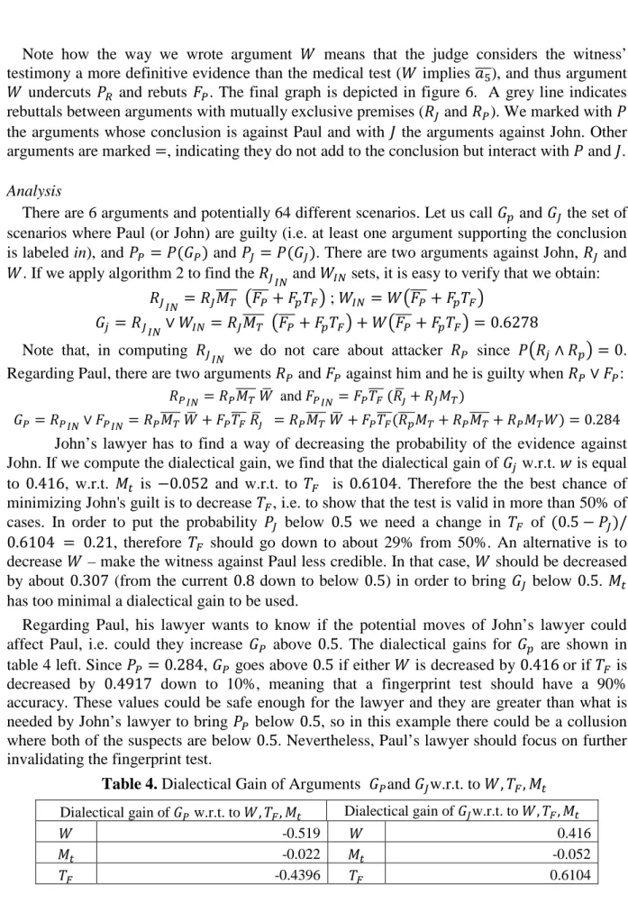
John’s lawyer has to find a way of decreasing the probability of the evidence against John. If we compute the dialectical gain, we find that the dialectical gain of %_W w.r.t. ² is equal to 0.416, w.r.t. Ä_t is −0.052 and w.r.t. to Ê_Ë is 0.6104. Therefore the the best chance of minimizing John's guilt is to decrease Ê_Ë, i.e. to show that the test is valid in more than 50% of cases. In order to put the probability _Ã below 0.5 we need a change in Ê_Ë of 0.5 − _Ã /

0.6104 = 0.21, therefore Ê_Ë should go down to about 29% from 50%. An alternative is to decrease ³ – make the witness against Paul less credible. In that case, ³ should be decreased by about 0.307 (from the current 0.8 down to below 0.5) in order to bring %_Ã below 0.5. Ä_t has too minimal a dialectical gain to be used.

Regarding Paul, his lawyer wants to know if the potential moves of John’s lawyer could affect Paul, i.e. could they increase %_› above 0.5. The dialectical gains for %_f are shown in table 4 left. Since _› = 0.284, %_› goes above 0.5 if either ³ is decreased by 0.416 or if Ê_Ë is decreased by 0.4917 down to 10%, meaning that a fingerprint test should have a 90% accuracy. These values could be safe enough for the lawyer and they are greater than what is needed by John’s lawyer to bring _› below 0.5, so in this example there could be a collusion where both of the suspects are below 0.5. Nevertheless, Paul’s lawyer should focus on further invalidating the fingerprint test.

Table 4. Dialectical Gain of Arguments %_›and %_Ãw.r.t. to ³, Ê_Ë, Ä_t

Dialectical gain of %_› w.r.t. to ³, Ê_Ë, Ä_t Dialectical gain of %_Ãw.r.t. to ³, Ê_Ë, Ä_t

³ -0.519 ³ 0.416

Ät -0.022 Ät -0.052

RELATED WORKS

The idea of merging probabilities and abstract argumentation was first presented by Dung et al. [3], and a more detailed formalization was provided by Li et al. [4], along with the works by Hunter [6] and Thimm [14]. In Li et al.’s definition is not a joint probability but a scalar function → [0,1] and a similar scenario-like approach (extension-based rather than argument-based) is used. Li et al.’s work is limited to fully independent arguments with grounded semantics, and no exact computation behind the brute force algorithm is analyzed ,while our paper also considers preferred semantics, providing an algorithm to compute and studying the behavior of w.r.t. to reinstatement, accrual, and response to changes.

Thimm in [14],and Hunter [6] in his epistemic approach, start from a complementary angle. Both authors assume that there is already an uncertainty measure – potentially not probabilistic – defined on the admissibility set of each argument (i.e. _>? is given as a function

>?: → [0,1]). Starting from >? rather than poses the question: which >? assignments

are acceptable? The authors both argue that only a subset of these measurements can be sensibly associated with an argumentation framework. They define a series of rules to identify a rationally acceptable probability distribution of _>?, such as the rationality and p-justifiability properties. In our paper we follow a complementary approach, since our aim is to start from (assumed to be a probability measure) and then compute _>?.

Regarding other works investigating gradualism in argumentation, we first mention Pollock’s work on degrees of justification [9]. Pollock rejects the use of probabilities to propagate numerical values on an argumentation framework, but he considers probabilities the only valid proxy for argument strength, and he uses the statistical syllogism as the standard comparison to measure strengths. Pollock considers the strengths of arguments as cardinal quantities that can be subtracted. The accrual of arguments is denied (except for a rebutting and an undercutting argument) and it is the argument with the maximum strength that defines the attack. In an argument chain, it is the argument with minimum strength that defines the strength of the conclusions. The model proposed by Cayrol and Dupin de Saint-Cyr [5] infers a measure of argument strengths from their position in the argumentation framework. This extrinsic strength cannot be mapped to probability or beliefs, and leads to an ordering on the arguments that does not fit our problem. The vs-defence model, by Cayrol and and Lagasquie-Schiex [1], is an extension of AF where attacks have a strength associated with them. Argument admissibility status is the result of the comparisons of attack strengths. We have seen two main problems: there is no description about how to compute such a strength, how to practically set a priority level and a preferral order, as Pollock wrote in [9]: if we were to be serious about arguments' strength, there must be a way to measure it.

In [1], the authors propose an argumentation framework with various degrees of attacks. They extend a work by Martinez & Garcia [12] that first extended Dung’s argumentation framework, introducing different levels of attacks. The work contributes to the development of argumentation with attacks of different strength. [8] was the first research to suggest the use of weights both on arguments and on attacks and Dunne et al. [11] have proposed weighted argument systems in which attacks have a numeric weight, indicating how reluctant one would be to disregard the attack. They accept that attacks can have different weights, and such weights might have different interpretations: an agent-based priority voting, or a measure of how many premises of the attacked argument are compromised.

CONCLUSIONS AND FUTURE WORKS

We have analyzed probabilistic argumentation frameworks and provided a first recursive algorithm to compute the probability of argument acceptance. We also studied various properties such as sensitivity to changes and behavior in the presence of reinstatement, accruals and cycles. We showed how PAF can be used as a tool to argue with probabilistic information. Our results could be used by agents involved in a discussion, in order to select the best move in a dialectical process or to analyze the sensitivity of the conclusions found. We believe that this is a contribution to the debate about gradualism in argumentation to justify further research in the theoretical and applicative studies of . Future developments may lie in the extension to other forms of uncertainty such as possibility or fuzzy/multi-value logic. Much work has to be done on the computational aspects and optimization of the recursive algorithm proposed, and an evaluation of its efficacy against a baseline brute-force approach.

References

1. C. Cayrol, C. D. Lagasquie-Schiex. "Acceptability semantics accounting for strength of attacks in argumentation,"19th ECAI, pages 995-996. Lisbon, Portugal, 2010

2. P. Dung, “On the acceptability of arguments and its fundamental role in nonmonotonic reasoning, logic programming and n-person games,” Artificial Intelligence, vol. 77, pp. 321–357, 1995

3. P. Dung, P. Thang. "Towards (Probabilistic) Argumentation for Jury-based Dispute Resolution," COMMA 2010. IOS Press, 171-182

4. Hengfei L., N. Oren, T. J. Norman. Probabilistic Argumentation Frameworks. 1st TAFA, JICAI 2011, Barcelona, Spain

5. C. Cayrol, F. Dupin de Saint-Cyr (2010) "Change in Abstract Argumentation Frameworks: Adding an Argument", Vol. 38, 49-84

6. Hunter, A. "A probabilistic approach to modelling uncertain logical arguments." International Journal of Approximate Reasoning (2012).

7. Caminada, M.W.A., and D.M. Gabbay. "A logical account of formal argumentation." Studia Logica 93.2-3 (2009): 109-145.

8. Barringer H., D. Gabbay, “Temporal dynamics of support and attack networks,” Mechanizing Mathematical Reasoning. LNAI 2605. Springer, 2005, 59–98.

9. Pollock, J., "Defeasible reasoning with variable degrees of justification,", 2001 Artificial Intelligence, Vol 133, Pg. 233-282.

10.Prakken, Henry. "An abstract framework for argumentation with structured arguments." Argument and Computation 1.2 (2010): 93-124.

11.Dunne, P.E., A. Hunter, P. McBurney, S. Parsons, “Inconsistency tolerance in weighted argument systems,” in Proc of AAMAS, 2009.

12.Martinez, D.C., A. J. Garcia, “An abstract argumentation framework with varied-strength attacks,” in Proc of KR, 2008, pp. 135–143.

13.Vreeswijk, G. "Abstract argumentation systems," Artificial Intelligence 90, 225–279, 1997 14.Thimm, M. "A Probabilistic Semantics for abstract Argumentation," ECAI. 2012.