See discussions, stats, and author profiles for this publication at: https://www.researchgate.net/publication/320665899
Iterated-greedy-based algorithms with beam search initialization for the
permutation flowshop to minimise total tardiness
Article in Expert Systems with Applications · October 2017
DOI: 10.1016/j.eswa.2017.10.050 CITATIONS 14 READS 142 3 authors, including:
Some of the authors of this publication are also working on these related projects:
Collaboration strategies in de centralized supply chains with partial information sharingView project
Models and algorithms for the order scheduling problems considering setup timesView project Victor Fernandez-Viagas Universidad de Sevilla 34PUBLICATIONS 401CITATIONS SEE PROFILE Jose M. Framinan Universidad de Sevilla 188PUBLICATIONS 3,131CITATIONS SEE PROFILE
Iterated-greedy-based algorithms with beam search
initialization for the permutation flowshop to minimise
total tardiness
∗
Victor Fernandez-Viagas
1†, Jorge M. S. Valente
2, Jose M. Framinan
11 Industrial Management, School of Engineering, University of Seville,
Camino de los Descubrimientos s/n, 41092 Seville, Spain, {vfernandezviagas,framinan}@us.es
2 LIAAD - INESC TEC, Faculdade de Economia, Universidade do Porto, Porto, Portugal, [email protected]
November 1, 2017
Abstract
The permutation flow shop scheduling problem is one of the most studied op-erations research related problems. Literally, hundreds of exact and approximate algorithms have been proposed to optimise several objective functions. In this pa-per we address the total tardiness criterion, which is aimed towards the satisfaction of customers in a make-to-order scenario. Although several approximate algorithms have been proposed for this problem in the literature, recent contributions for related problems suggest that there is room for improving the current available algorithms. Thus, our contribution is twofold: First, we propose a fast beam-search-based con-structive heuristic that estimates the quality of partial sequences without a complete evaluation of their objective function. Second, using this constructive heuristic as initial solution, eight variations of an iterated-greedy-based algorithm are proposed. A comprehensive computational evaluation is performed to establish the efficiency of our proposals against the existing heuristics and metaheuristics for the problem. Keywords: Scheduling, Flowshop, Heuristics, PFSP, tardiness, beam search, iter-ated greedy algorithm, iteriter-ated local search
∗Preprint submitted to Expert Systems with Applications. http://dx.doi.org/10.1016/j.eswa.2017.10.050 †Corresponding author. Email: [email protected]
1
Introduction
The flow shop is a common manufacturing layout in which a set ofnjobs has to be processed in a
set ofmmachines where each job follows the same route through the machines. For simplicity, the
problem is denoted by permutation flow shop (PFSP in the following) when the same sequence of jobs is applied on each machine. The PFSP is one of the most studied optimization problems in Operations Research. Among the objectives studied in the literature (see e.g. Pan and Ruiz, 2013; Fernandez-Viagas and Framinan, 2014; Fernandez-Viagas et al., 2016a), the minimisation of the total tardiness is essential for manufacturing systems (Raman, 1995), since due dates play an important role in these systems (Panwalkar et al., 1982) and delays may increase costs and/or the dissatisfaction of customers (resulting in either a poor reputation, or even the loss of customer) (Sen and Gupta, 1984).
According to theα|β|γ notation (see e.g. Pinedo, 1995), the PFSP to minimise total tardiness
can be denoted asF m|prmu|P
Tj. Since this problem is known to be NP-hard (Du and Leung,
1990), during the last years several approximate algorithms –heuristics and metaheuristics– have been proposed in the literature (see e.g. Vallada et al., 2008; Li et al., 2015; Karabulut, 2016). However, these proposals have not been compared against themselves, or the comparison has not been carried out under the same conditions, so the state-of-the-art regarding approximate algorithms for the problem remains unclear. Instead, these methods have been usually compared against either the genetic algorithm proposed by Vallada and Ruiz (2010), the Iterated Greedy (IG) algorithm by Ruiz and Stützle (2007), and/or the NEHedd by Kim (1993), which is the adaptation for the problem of the well-known NEH heuristic by Nawaz et al., 1983. The latter two are considered key methods in the flowshop scheduling literature since the noteworthy papers by Nawaz et al. (1983) and Ruiz and Stützle (2007), respectively. Regarding the NEHedd, it is probably the key constructive heuristic for the problem due to several reasons (Fernandez-Viagas and Framinan, 2015d): aside being an efficient heuristic for the problem, it is used to obtain an initial solution by the rest of efficient constructive or improvement heuristics, and by more than half of the efficient improvement heuristics or metaheuristics. Regarding IG, it remains the cornerstone of subsequent algorithms in the flowshop literature and can be considered as
the state-of-the-art algorithm for several scheduling problems (see e.g. Fernandez-Viagas and
Framinan, 2015b and Dubois-Lacoste et al., 2017)1.
Despite the preeminence of these two algorithms, recent advances in related scheduling prob-lems have shown that they can be improved: On the one hand, some studies (see e.g. Dong et al., 2009 and Pan and Ruiz, 2014) have found better results by varying the destruction-construction phase in the IG for total flowtime minimisation, which is related to the problem under consid-eration (see Fernandez-Viagas and Framinan, 2015d). On the other hand, recent constructive heuristics based on a non-complete evaluation of the partial sequences have clearly outperformed the original NEH for other objective functions (see e.g. Fernandez-Viagas and Framinan, 2015c; Fernandez-Viagas et al., 2016a; Fernandez-Viagas and Framinan, 2017).
To tackle the aforementioned issues, the contribution of this work is twofold: We first im-plement a beam search algorithm for the problem which constructs several partial sequences in parallel. The algorithm estimates the value of the objective function for each partial sequence based on specific variables of the problem. We then develop several iterated-greedy-based algo-rithms to improve the pool of sequences generated by the beam search algorithm. To explore the effect of the construction phase in the algorithm, we implement eight different methods based on insertions, exchanges, randomness and optimizations of partial solutions. We finally compare the proposals with the best performing algorithms in the literature in an exhaustive computational evaluation.
The remainder of the paper is as follows: In Section 2 we formalise the problem and discuss its background. In Section 3 we propose the beam search and the iterated-greedy-based algorithms. These algorithms are compared with the state-of-the-art methods in Section 4. Finally, in Section 5 we discuss the main conclusions of the paper.
1IG is currently a state-of-the-art algorithm for makespan minimisation (F m|prmu|C
max). As stated
by Fernandez-Viagas et al. (2017), the speed up proposed by Taillard (1990) is probably one of main reason of the good-performance of insertion phases -constructing jobs following a greedy method for that scheduling problem- as compared to randomized ones.
2
Problem Statement and Background
The problem under study can be set as follows: a set N of n jobs have to be processed in
a flowshop composed of a set M of m machines. Each job j ∈ {1, . . . , n} has a due date dj
and a processing time pij on each machine i ∈ {1, . . . , m}. Given a sequence of jobs Π :=
(π1, . . . , πr, . . . , πn) where r ∈ {1, . . . , n} is an index of the position in a sequence, let Cij(Π)
(abbreviated toCij whenever it does not lead to confusion) be the completion time of jobj on
machineiaccording to sequence Π. Obviously,Cmj(Π) is the completion time of jobjon the last
machine, and Cmπn(Π) =Cmax is the maximum completion time or makespan of the sequence.
The tardiness (earliness) of jobj is defined asTj = max{Cmj−dj,0}(Ej = max{dj−Cmj,0}).
Analogously, total tardiness, whose minimisation is the goal of our problem, is defined asP
Tj =
Pn
j=1max{Cmj−dj,0}, while total earliness is defined asPEj =Pnj=1max{dj−Cmj,0}. Note
that the completion times can be computed recursively as follows:
Ciπj =max{Ci−1,πj, Ci,πj−1}+piπj (1)
where C0πj =Ciπ0 = 0.
A number of approximate procedures have been proposed in the literature to provide good solutions for this problem in reasonable computation times. A review and evaluation of these algorithms prior to 2008 is given in Vallada et al. (2008). From this review, it turns out that the NEHedd proposed by Kim (1993), the ENS2 by Kim et al. (1996), and the simulated annealing algorithms by Hasija and Rajendran (2004) and Parthasarathy and Rajendran (1997) (denoted as HR and SAH, respectively) are the most promising algorithms for the problem. Using the same computer conditions, Framinan and Leisten (2008) propose a hybrid algorithm (denoted as
HA) which outperforms both the HR and the SAH0 (proposed by Parthasarathy and Rajendran,
1998)2. This algorithm combines the iterated greedy and the variable neighbourhood search
algorithms using a partial (adjacent-pairwise-exchange) local search in its construction phase, as well as an insertion local search improvement. In addition, Framinan and Leisten (2008) have 2This SAH0 algorithm was not included in the computational evaluation of Vallada et al. (2008) due
also proposed a speed up mechanism to decrease the complexity of the evaluation3. Recently, Karabulut (2016) have found around 50% time saving when applying it to the NEH.
In parallel to the contribution by Framinan and Leisten (2008), Vallada and Ruiz (2010) propose three genetic algorithms (GAPR, GAPR2, and GADV) that also outperform the HR and SAH in a fair comparison, and using a similar speed up mechanism for the problem. The best results were obtained by the GAPR version, although this algorithm was not compared
to HA. Laterly, several contributions have outperformed the GAPR algorithm. First, Cura
(2015) proposes an evolutionary algorithm (EA in the following), that outperforms both GAPR and SAH. The algorithm includes a mating procedure to diversify the solutions. Two local search methods with different neighbourhood sizes are employed, although the comparison is not performed using the same conditions, i.e. the algorithms used for comparison were not re-implemented. Secondly, several trajectory scheduling methods are proposed by Li et al. (2015)
using six different composite heuristics (denoted as CHi) and three perturbation methods. Let
us denote as TSMij the trajectory scheduling methods composed of composite heuristic CHi and
perturbation methodj. Among these methods, the best results are found by TSM63. On the one
hand, under the same stopping criterion and the same computer conditions, TSM63 outperforms
the three genetic algorithms by Vallada and Ruiz (2010), i.e. GAPR, GAPR2, and GADV. On the other hand, the proposed composite heuristics outperform the NEHedd but require additional CPU times. Regarding NEHedd, Fernandez-Viagas and Framinan (2015d) analyse the structure of the problem, finding that there are a high number of ties in the selection procedure of NEHdd. Eight tie-breaking mechanisms are then proposed and compared with the original one, resulting that each tie-breaking mechanism (with the exception of the random one) statistically
outperforms NEHedd. The most promising tie-breaking mechanisms are NEHedd(TBIT1) and
NEHedd(TBMS-Taillard, IT1) (these heuristics are denoted in the following as TBIT1 and TBTa,
3The speed up mechanism is a very common practice in the flowshop layout with permutation
se-quences. Taillard (1990) have proposed the first one for F m|prmu|Cmax. Since then, several other
mechanisms have been proposed for different constraints and/or objectives. Naderi and Ruiz (2010), Rios-Mercado and Bard (1998) and Fernandez-Viagas and Framinan (2015b) have successfully adapted them for theDF|prmu|Cmax,F m|sijk, prmu|CmaxandF m|prmu|(Cmax/Tmax) problems, respectively. With
some modifications and lesser decrease in CPU times, they have been also adapted for theF m|prmu|P
Cj, F m|prmu|P
Tj, F m|prmu|PEj+PTj and F m|block|PCj problems by Li et al. (2009), Framinan
respectively). In addition, they also statistically improve GAPR when used as an initial solution instead of the traditional NEHedd.
Recently, Karabulut (2016) propose KIG, an iterated greedy algorithm that incorporates a random local search method instead of the traditional insertion local search method. The search randomly performs insertion and exchanges using the speed up mechanism proposed by
Framinan and Leisten (2008), until no more improvement is achieved inniterations. In addition,
it uses a simple annealing-like acceptance criterion with a constant temperature based on the makespan and the due dates of the jobs. Although the authors do not compare their proposal with algorithms specifically developed for the problem, they compare it with the original iterated greedy algorithm proposed by Ruiz and Stützle (2007) –originally designed for the PFSP to minimise makespan–, which has been reimplemented for the problem under consideration. It is to note that such iterated greedy algorithm was found to be outperformed by GAPR for the problem under study.
To summarise, several algorithms have been proposed in the literature to solve the problem under consideration. However, the new picture of the efficient metaheuristics for the problem remains unclear due to the following issues:
1. The most promising metaheuristics found by Vallada et al. (2008) have been outperformed by GAPR and HA, but there is no comparison among these two latter algorithms and, to the best of our knowledge, contributions after 2008 do not include HA in their comparisons.
2. There is no computational comparison among the recent iterative algorithms proposed in
the literature, i.e. EA, TSM63, and KIG.
3. Some metaheuristics are tested either under different computer conditions or versus non-state-of-the-art metaheuristics (see e.g. Cura, 2015; Karabulut, 2016).
In this paper, in Section 3 we first propose both a beam search algorithm with a fixed stopping criterion, and a set of eight different iterated-greedy-based algorithms varying their construction phase. In addition, we perform a comprehensive computational evaluation of the heuristics and metaheuristics in Section 4. By doing so, we establish the set of efficient algorithms for the problem.
3
Proposed algorithms: beam search and
iterated-greedy-based algorithms
In this section, we propose several approximate procedures to solve the problem. The first
proposal is a population-based constructive heuristic, which constructs several partial sequences in parallel, appending jobs, one by one, at the end of the sequences (see Subsection 3.1). Secondly,
we propose several iterative improvement algorithms based on a single solution. Using the
previous heuristic as initial solution, these algorithms iteratively search for the local optimum of a sequence obtained by a destruction-construction-based phase (see Subsection 3.2). Note that the division between heuristics and metaheuristics is unclear in the literature and several classifications have been proposed (see e.g. Zanakis et al., 1989; Zäpfel et al., 2010). In this paper, we adopt the same definition as in Ruiz and Maroto (2005) and Fernandez-Viagas et al. (2017), where metaheuristics are defined as iterative improvement algorithms with stopping criteria depending on CPU time or number of iterations. In contrast, heuristics naturally stop when their steps are finished.
3.1
Beam search algorithm
In this subsection we present a beam search algorithm, denoted by BS(γ), with an advance
prior-ity evaluation function. Similarly to the B&B algorithm, this approximate procedure constructs a search tree, where each node is formed by a partial sequence and the child nodes are obtained by adding one of the unscheduled jobs at the end of the parent node. However, only the most
γ promising nodes (denoted as beam width in the following) are kept for the next iteration.
Beam search has been successfully applied to several scheduling problems in the literature (see e.g. Valente and Alves, 2005, 2008). Traditionally, two different functions have been applied to evaluate the nodes (Valente, 2010):
• Priority evaluation function. The node is evaluated by estimating the influence of the
last job in the partial sequence. This evaluation of just one job in the node (omitting the influence of the other jobs) implies both that computing this function requires a low
complexity order and that it is node-dependent, i.e. only children from the same parent node can be compared.
• Total cost evaluation function. The final objective function value to be achieved for this
node is estimated taking into consideration all unscheduled jobs. Obviously, this function
is node-independent as complete sequences are estimated. In addition, its complexity
increases significantly.
Recently, Fernandez-Viagas et al. (2016b) and Fernandez-Viagas and Framinan (2017) have achieved excellent results using a node-independent priority evaluation function. The idea is
to assign to each node a “genetic” code which keeps the historical behaviour of that node. By
means of both this code and the influence of the last element, child nodes from different parents can be compared. This approach is applied in our proposal.
The proposed beam search algorithm is composed of several nodes in n different levels. Let
us denote by Slk the partial sequence of the lth node in iteration k, withl ∈ [1, γ]. Each node
is then formed by a partial sequence Slk, Slk := (sk1,l, ..., skk,l), of k jobs, and by a set Uk
l (with
Uk
l := {uk1,l, ..., unk−k,l}) of n−k unscheduled jobs. Whenever it does not lead to confusion, let
us also denote that node by Slk. For each iteration k, n−k child nodes are created from each
partial sequenceSk
l by adding one job from set Ulk at the end of the sequence. The bestγ child
nodes are selected to be the partial sequences of the nodes for the next iteration, i.e. Slk+1,
∀l∈ {1, ..., γ}. More specifically, the steps of the proposed algorithm are as follows:
Step 1 Initialization
Step 2 While k= 2, . . . , n−1, repeat:
Step 2.1 Branching
Step 2.2 Node evaluation
Step 2.3 Node selection
Step 3 Final evaluation
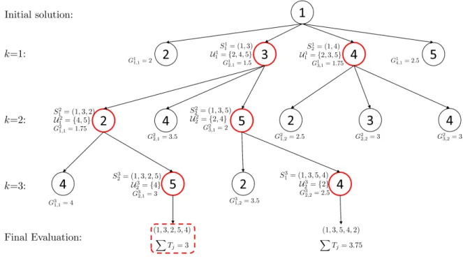
To clarify both the branching and candidate selection phases, a simple example with five jobs
Figure 1: Example of BS
Next, each phase is explained in more detail:
• Initialization (Step 1). The first node is formed by job j∗ with the minimum sum of
completion time on the last machine and weighted idle times,wj. Let us denote such sum
as indexξj, i.e. j∗:= arg minj{ξj}where:
ξj := m X i=1 pij +wj = m X i=1 pij + (n−2) 4 · m X i=2 m·Pi−1 i0=1pi0j i−1 ! , ∀j∈[1, n] (2)
In case of ties, the job with minimumwj is chosen. See Liu and Reeves (2001),
Fernandez-Viagas et al. (2016b), and Fernandez-Fernandez-Viagas and Framinan (2017) for similar initializations.
• Branching (Step 2.1). Each nodeSlk is branched to form n−kchild nodes. Child node v
(with v∈[1, n−k]) is constructed from the node by addingukv,l at the end of the partial
sequence Slk. Note that the number of child nodes in iteration kis γ(n−k).
• Node evaluation (Step 2.2). As mentioned before, the child nodes are evaluated according
– The “genetic” code. This first component measures the genetic offspring of the child node. By doing so, we are able to compare child nodes with different sequenced jobs,
i.e. from different nodes. Obviously, each one of the child nodes of node Slk has the
same genetic code.
– The influence of the last element. It measures the influence of the last job inserted
at the end of the partial sequence.
In order to define both influences, we explore the specific characteristics of the problem.
Regarding the genetic code of node Slk, its goal is twofold. On the one hand, it should
consider the contribution of the partial sequence to the objective function. As jobs in the following iterations are added always at the end of the partial sequence, the total tardiness of the jobs in the partial sequence stays unalterable until the end. On the other hand, it should address the indirect influences on the objective function of the future jobs to be added to the partial sequence. These influences make possible to compare child nodes of different offspring. To achieve these goals, the genetic code incorporates the following aspects which may be considered and balanced:
1. Cumulative total tardiness (T T). It represents the total tardiness of partial sequences
Sk+1
l0 . Note that S
k+1
l0 represents the l
0
th best node of iteration k+ 1 formed by
appending job ukv,l at the end of node Slk. As l and l0 are not necessarily the same
nodes, let us denote by job[l0] such job uv,lk and by branch[l0] such l. Then the
cumulative total tardiness of Sk+1
l0 is computed as follows: T Tk+1 l0 =T T k branch[l0]+T k job[l0],branch[l0], ∀k={2, . . . , n−1}, l 0 ={1, . . . , γ} (3)
where Tjlk is the tardiness of job j of nodeSlk in iteration k.
2. Cumulative total earliness (T E). Analogously, it represents the total earliness of
partial sequencesSk+1
l0 . Denoting byE
k
jlthe earliness of jobjof nodeSlk in iteration
k, the cumulative total earliness of node Sk+1
T Elk0+1=T Ebranchk [l0 ]+E k job[l0],branch[l0], ∀k={2, . . . , n−1}, l 0 ={1, . . . , γ} (4)
3. Cumulative weighted idle time (T I). It represents the cumulative weighted idle time
of each job of partial sequence Sk+1
l0 , which is defined by:
T Ik+1 l0 =T I k branch[l0]+I k job[l0],branch[l0], ∀k={2, . . . , n−1}, l 0 ={1, . . . , γ} (5)
whereIjlk is the weighted idle time between the last job of sequenceSlk and jobj, which is
inserted in the last position of the sequence, see Equation (6).
Ijlk = m X i=2 m·max{Ci−1,j−Ci,[k],0} i−1 + (k−1)·(m−i+ 1)/(n−2) (6)
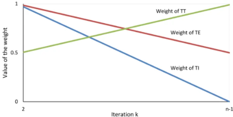
Note that, after the node selection phase, the cumulative total tardiness, total earliness and weighted idle time are updated by incorporating the corresponding value of the last job. Thereby, it avoids to completely re-calculate of them in each iteration. Obviously, the influence of the cumulative total tardiness increases when the sequence contains more jobs, while the weight of the indirect influence (i.e. the cumulative total earliness and idle time) decreases with each iteration. More specifically, in the first iterations of the algorithm, it seems better to choose sequences with high values of total idle times and total earliness times to have more promising partial sequences for the next iterations. In contrast, in the last iterations, the influence of the total tardiness becomes more relevant
as objective function of the problem. AmongT E and T I, the total earliness seems to be
a better estimation of the tardiness of the unscheduled jobs in these last iterations. In
addition, by keepingT E in the last iterations, we break the greedy behaviour of the total
tardiness. To deal with these issues and after some preliminary tests, we propose weights for the three components following the simple linear functions shown in Figure 2.
Figure 2: Values of the weights of total tardiness, total earliness, and total weighted idle
time, depending of the iteration k.
Hence, the genetic code, denoted asFk
l0, of nodel
0
in iterationkhas the following
expres-sion: Flk0 =T Ik l0· n−k−1 n +a·T E k l0· 2n−k−1 2n +b·T T k l0· k−1 +n 2n , ∀k={2, . . . , n−1}, l 0 ={1, . . . , γ} (7)
whereaandbare parameters of the algorithm to balance the contribution of T I,T E and
T T. Implicitly, low values for aand bindicate that the contribution of T I is higher than
T E and T T. So, in order to reduce the number of parameters of the algorithm, only a
and b (forT E and T T, respectively) are considered, and the influence of T I is measured
varying this parameter asT I was normalized.
Regarding the index, denoted as Lkvl, employed to estimate the contribution of the last
job, uk
vl, when evaluating child node v of node Slk, we follow a similar procedure to the
genetic code, where the weighted idle time and the earliness time are chosen as criteria. Note that the influence of the tardiness of the last job is included in the earliness since a tardy job indicates an earliness equals to 0. In addition, once several jobs are tardy, they stay tardy in the following iterations and the influence of other elements should be taken into account to choose the job. Regarding these other elements, several studies (see e.g. Liu and Reeves, 2001; Fernandez-Viagas and Framinan, 2015c) found excellent results by incorporating an estimation of the contribution of the unscheduled jobs. To deal with that,
we add the total tardiness of all jobs ukvl,∀v ∈1, ..., n−k, denoted by Wlk. Note that job
ukvl is also included inWlkindex of child nodev. By doing so, we reduce the computational
effort of this index. Hence, indexLkvl can be defined by Expression (8), wherecand eare
parameters of the algorithm again to balance the contributions ofEukk
vl,l
andWlk. Similarly
toFk
l0, after a preliminary test, we use a decreasing function for the weight of the idle time,
and an increasing one for Wlk (the tardiness of the unscheduled jobs is closer to the real
one in the last iterations than in the first ones).
Lkvl = (n−k−1)·Iukk vll +c·Eukk vl,l + e n−k+ 1·W k l , ∀k={2, . . . , n−1}, l ={1, . . . , γ}, v ={1, . . . , n−k} (8)
Then, each child node v obtained by node Slk is computed using index Gkvl which adds
both contributions:
Gkvl =Flk+Lkvl, ∀k={2, . . . , n−1}, l={1, . . . , γ}, v={1, . . . , n−k} (9)
• Node selection (Step 2.3). Among theγ(n−k) child nodes in iterationk, the bestγ ones
are kept as the set of nodes of iterationk+ 1. More specifically, in iterationk, theγ nodes
with the lowest values of theGkvl indicator (∀v∈ {1, . . . , n−k}, l∈ {1, . . . , γ}) are selected
for the next iteration.
• Final evaluation (Step 3). The total tardiness of the nodes selected in the last iteration, i.e.
nodesSln−1(∀l∈1, ..., γ), is evaluated. The sequence yielding the minimal total tardiness
is the final sequence of the beam search algorithm.
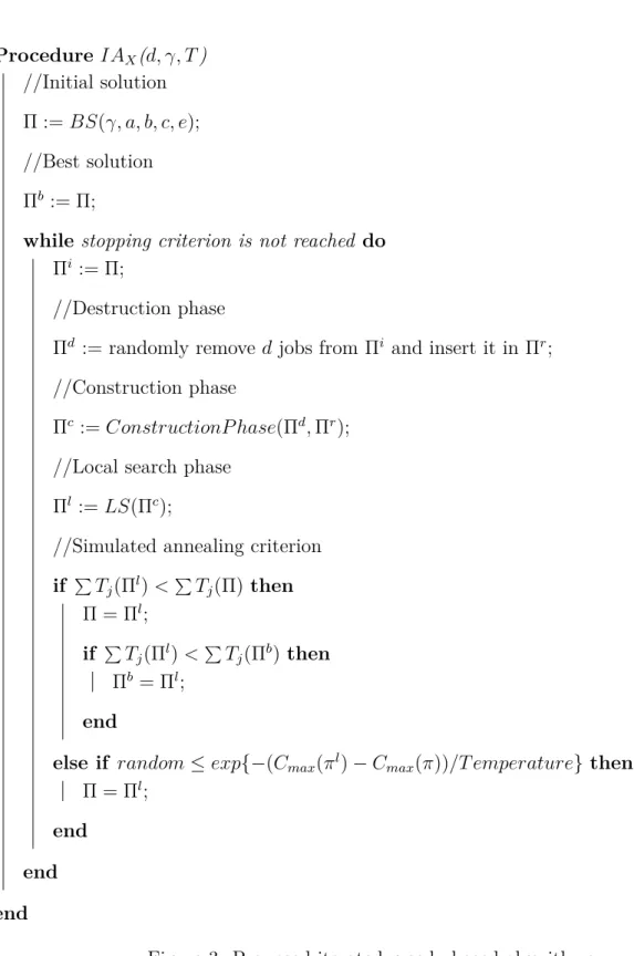
3.2
Iterated-greedy-based algorithms, IA
The iterated greedy algorithm is a single-solution-based metaheuristic, originally proposed for flow-shop-type scheduling problems by Ruiz and Stützle (2007). Starting with an initial solution, this metaheuristic iteratively perturbs a sequence and searches for its local optimum. Then, the
iterated greedy algorithm destructs several jobs of a sequence in each iteration, and constructs
them following a greedy approach. More specifically, in a destruction phase,djobs are randomly
removed from the iteration sequence, denoted as Πi. Let us denote by Πr, Πr := (π1r, . . . , πdr), the
sequence formed by the removed jobs and by Πd the partial sequence of lengthn−d, formed by
Πiwithout the removed jobs. After that, in a construction phase, each job in Πris inserted in the
position of Πdyielding the lowest value of the objective function. Πcis the so obtained sequence.
Finally, this metaheuristic looks for the local optimum of the constructed sequence and performs a basic simulated annealing phase. In this subsection we propose eight simple Iterated Algorithms
based on the iterated greedy metaheuristic4, denoted as IA, consisting on the following same four
phases which are repeated until a stopping criterion is reached: destruction phase; construction phase; local search phase; and a simple simulated annealing phase. As described earlier, the destruction-construction phase plays an important role in the efficiency of the metaheuristic. In order to take it into account, in this paper we propose and compare the following eight different procedures:
1. Random insertion (let us denote by IARI the proposed algorithm using this construction
phase) This procedure replaces the greedy insertion of the traditional iterated greedy by
a random one. More specifically, each removed job πir, ∀i∈1, . . . , d, is randomly inserted
in Πd.
2. Greedy insertion (IAGI). This is the traditional construction phase of the iterated greedy
algorithm, i.e. each removed jobπir,∀i∈1, . . . , d, is inserted in the position of Πdyielding
the lowest total tardiness.
3. Random general swap (IARGS). This procedure replaces the destruction and construction
phase of the algorithm by performing d random exchanges between jobs, i.e., d jobs are
randomly chosen from Πi and exchanged with other jobs of this sequence.
4Note that the iterated greedy algorithm is closely related to the iterated local search and in fact, it
could be considered as a special case of the iterated local search. This latter algorithm begins with an initial solution and iteratively modifies the current solution and looks for its local optimum. Therefore, assuming that a special type of modification of a solution is to perform the destruction and construction phase of the iterated greedy, both algorithms would be considered the same metaheuristic. However, in order to maintain the coherence with previous proposals in the literature, we also use the term “iterated-greedy-based algorithm” in the notation of our proposals.
4. Greedy general swap (IAGGS). In this procedure, a job is randomly chosen from Πi and
exchanged with each job of the sequence. Sequence Πi is replaced by the exchange yielding
the lowest total tardiness. The procedure is repeateddtimes for ddifferent jobs.
5. Random adjacent swap (IARAS). This procedure randomly chooses a job and exchanges
it with the next job of the sequence. The procedure is repeateddtimes.
6. Greedy insertion + Partial adjacent-swap-based local search method (IAGI_ALS). This
procedure is based on Framinan and Leisten (2008). Thereby, each job removedπri,∀i∈
{1, . . . , d} is inserted in the position of Πd yielding the lowest total tardiness (denoted as
positionb), as in the greedy insertion procedure. After that, an adjacent pairwise exchange
is performed for the jobs between the last position of the partial sequence and position b+ 1.
7. Insertion-based Local search + Greedy insertion (IAILS_GI). This procedure adapts the
procedure of destruction and construction proposed by Dubois-Lacoste et al. (2017). The
method performs an insertion-based local search on the partial sequence Πd, i.e. each job
of the sequence is removed and inserted in the best position. The procedure is repeated until there is no improvement in a complete iteration. The best sequence found by the
algorithm replaces Πd. After that, the traditional construction phase (i.e. greedy insertion)
is applied.
8. Greedy insertion + Local search insertion(IAGI_ILS). This procedure is an adaptation of
the method proposed by Pan and Ruiz (2014) and Pan et al. (2017). Similarly as IAGI_ALS,
each removed jobπr
i,∀i∈ {1, . . . , d} is inserted in the positionbof Πdyielding the lowest
total tardiness. After that, jobs in positionsb−1 andb+ 1 are removed and reinserted in
the position yielding the lowest total tardiness.
After the destruction-construction procedure, a local optimum of sequence Πc is obtained
in the local search phase. This phase iteratively removes each job in sequence Πc and inserts
it in the position with the lowest vaue of the objective function. The phase is stopped after a complete iteration without any improvement. Finally, the simulated annealing-like acceptance
criterion proposed by Karabulut (2016) is applied due to its excellent performance. This simple
criterion is a variation of the proposal of Ruiz and Stützle (2007) for F m|prmu|Cmax, which
has been successfully applied to other several objectives and/or scheduling problems (see e.g. Fernandez-Viagas and Framinan, 2015a,b; Ribas et al., 2017). The criterion uses a constant
T emperaturewhich depends on parameterT of the algorithm:
T emperature=T ·
Pn
j=1(LBCmax −dj)
n·10 (10)
where LBCmax is the lower bound of the makespan following the procedure established by
Taillard (1993). The pseudo-code of the proposed metaheuristic is shown in Figure 3. Note that BS is used as the initial solution of the proposed iterated-greedy-based algorithms.
ProcedureIAX(d, γ, T) //Initial solution Π :=BS(γ, a, b, c, e); //Best solution
Πb := Π;
while stopping criterion is not reached do
Πi := Π;
//Destruction phase
Πd := randomly remove d jobs from Πi and insert it in Πr;
//Construction phase
Πc:=ConstructionP hase(Πd,Πr); //Local search phase
Πl :=LS(Πc);
//Simulated annealing criterion
if P Tj(Πl)<PTj(Π)then Π = Πl; if P Tj(Πl)<PTj(Πb)then Πb = Πl; end
else if random≤exp{−(Cmax(πl)−Cmax(π))/T emperature} then
Π = Πl;
end end end
4
Computational Experience
In this section we compare the state-of-the-art algorithms against our proposals. Prior to per-forming this computational evaluation, we establish the conditions adopted to achieve a fair comparison. Firstly, in Subsection 4.1 we present the sets of instances generated. Secondly, the measures to evaluate both the quality of the solutions and the computational requirements of each algorithm are shown in Subsection 4.2. Regarding our proposals, two full experimental parameter tunings are described in Subsection 4.3. Next, in Subsection 4.4, the state-of-the-art algorithms, which are fully re-implemented, are shown. We compare them against our proposals by carrying out two different computational evaluations for heuristics and metaheuristics, see Subsections 4.5 and 4.6, respectively.
4.1
Sets of instances
In this paper, two benchmark testbeds, denoted asβ1 andβ2, are generated for the experiments
of our study. β1 is used for the calibration of the parameters of the proposed algorithms. The
computational evaluations of both heuristics and metaheuristics are carried out on benchmarkβ2.
By doing so, we avoid an over calibration of the parameters of our algorithms in the benchmark of comparison.
• Benchmark β1: This benchmark is generated by the procedure described in Vallada
and Ruiz (2010). It contains 108 different sizes of the problem varying the
parame-ters n, m, T and R. Ten instances are generated for each combination of parameters
n∈ {50,150,250,350}, m∈ {10,30,50}, T ∈ {0.2,0.4,0.6}, andR∈ {0.2, .0.6,1.0}, i.e. a
total of 1,080 instances are generated in this benchmark. T andRare parameters to
gener-ate different types of due dgener-ates for each size of the problem (see Potts and Van Wassenhove, 1982). They generate the processing times and the due dates with a uniform distribution
[1,99] and [P ·(1−T −R/2, P ·(1−T+R/2], respectively, whereP is the lower bound
for the makespan proposed in Taillard (1993).
• Benchmarkβ2: This benchmark is composed of the 540 instances of Vallada et al. (2008).
{0.2,0.4,0.6}, andR∈ {0.2, .0.6,1.0}, with five instances for each combination. Processing
times and due dates are generated following the same distributions than in benchmarkβ1.
4.2
Performance indicators
In our study, two computational evaluations are carried out to compare the most promising heuristics and metaheuristics. As a result, 23 algorithms are tested. To conduct a fair comparison among them, the algorithms are compared under the same conditions. More specifically, the following aspects are considered:
• We use the same computer (an Intel Core i7-3770 with 3.4 GHz, 16 GB RAM, and with
Microsoft Windows 8.1 64 bit operating system).
• We re-code each algorithm using the same programming language (C# under Visual Studio
2013).
• We use the same computational skills, libraries and common functions.
• We use the same stopping criteria for each metaheuristic.
In addition, each algorithm typically requires a different CPU time and obtains a different solution. In order to compare both the quality of the solutions and the computational efforts of the implemented algorithms, the indicators for comparison have to be established. On the one
hand, heuristics are compared using the Average Relative Deviation Index (denoted asARDI1h
for heuristich) and the Average Relative Percentage computation Time (denoted asARP Th for
heuristichfollowing the recommendation established by Fernandez-Viagas and Framinan (2015c)
and Fernandez-Viagas et al. (2017) (see Equations 11 and 12, respectively). On the other hand,
metaheuristics are only compared using theARDI1h as the same CPU times are used.
ARDI1h = I X i=1 RDI1ih I , ∀h= 1, . . . , H (11) ARP Th = 1 + I X i=1 RP Tih I , ∀h= 1, . . . , H (12)
LetI be the number of instances, andHbe the number of considered heuristics. The Relative
Deviation Index of heuristich in instance i,RDI1ih, and the Relative Percentage computation
Time,RP T1ih, are defined by the following expressions, respectively:
RDI1ih= OFih−Besti W orsti−Besti , ∀i= 1, . . . , I, h= 1, . . . , H (13) RP Tih= Tih−ACTi ACTi , ∀i= 1, . . . , I, h= 1, . . . , H (14)
where Besti and W orsti are the best and worst known solution for one run in instance i5,
respectively. Let Tih and OFih be the CPU time and the objective function value obtained by
heuristic h in iteration i, respectively. Finally, ACTi is the average CPU time required by all
compared algorithms in iterationi, which is defined by:
ACTi =
PH
h=1Tih
H , ∀i= 1, . . . , I (15)
Regarding the experimental parameter tuning on benchmarkβ1, we apply a different indicator
of the quality of the solution. More specifically, we usedARDI2, which is a small modification
of ARDI1: ARDI2h = I X i=1 RDI2ih I , ∀h= 1, . . . , H (16) RDI2ih= OFih−Best 0 i W orst0i−Best0i, ∀i= 1, . . . , I, h= 1, . . . , H (17)
whereBest0i and W orst0i are the best and worst total tardiness among the algorithms tested
in the calibration, respectively.
5These values are presented as on-line materials, which are taken from
4.3
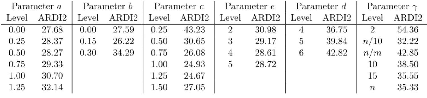
Experimental parameter tuning
In this subsection, two full factorial design of experiments are presented to determine the best combinations of parameters for the proposed algorithms. Both experiments are evaluated on
benchmark β1. Regarding BS, firstly four parameters (a, b, c and e) have been proposed to
balance the contributions in the evaluation of partial sequences. In addition, parameterγ (beam
width) directly influences its complexity,O(max{γ·n2·m, γ2·n2}), and consequently the CPU
time of the proposed beam search. For each value of γ, there is a trade-off between the quality
of solutions and the computational effort. Thus, this parameter is removed of this experimen-tal parameter tuning (see e.g. Liu and Reeves, 2001; Fernandez-Viagas and Framinan, 2015c; Fernandez-Viagas et al., 2016b for similar approaches) to avoid a calibration of each parameter
γ, and its value is set to 15. So the following levels of the parameters are tested:
• a∈ {0,0.25,0.5,0.75,1,1.25} • b∈ {0,0.15,0.3}
• c∈ {0.25,0.5,0.75,1,1.25,1.5}
• e∈ {2,3,4,5}
Regarding the proposed iterated-greedy-based algorithms, they use three parameters: d, γ,
and T. Firstly, we use in this test d ∈ {4,5,6} for the number of destructed jobs. Regarding
the parameter γ, the CPU time of IAi depends on its stopping criterion instead of γ, since
BS is applied as its initial solution. So, different values of γ only perturbs its objective
func-tion value, i.e. we may now measure the influence of γ in the quality of the solutions of the
metaheuristics without altering its CPU time. In this calibration test, we use the following
lev-els, γ ∈ {2, n/10, n/m,10,15, n}. For parameter T, we use the best value found by Karabulut
(2016), i.e. T = 1.0, since its influence has not been found to be statistically significant in several
previous studies (see e.g. Pan and Ruiz, 2014; Fernandez-Viagas and Framinan, 2015a). The
calibration test is carried out for IARI and using n·(m/2)·60 ms.
In this paper, we carry out two non-parametric Kruskal-Wallis analyses to determine the statistical differences between the levels of the parameters. Note that the normality and
ho-Parameter a Parameter b Parameter c Parameter e Parameter d Parameter γ
Level ARDI2 Level ARDI2 Level ARDI2 Level ARDI2 Level ARDI2 Level ARDI2
0.00 27.68 0.00 27.59 0.25 43.23 2 30.98 4 36.75 2 54.36 0.25 28.37 0.15 26.22 0.50 30.65 3 29.17 5 39.84 n/10 32.22 0.50 28.27 0.30 34.29 0.75 26.08 4 28.61 6 42.82 n/m 42.85 0.75 29.33 1.00 24.93 5 28.72 10 38.50 1.00 30.70 1.25 24.67 15 35.55 1.25 32.14 1.50 27.05 n 35.33
Table 1: Average results of RDI2 for each tested parameter.
moscedasticity assumptions were not satisfied. In addition, the indicatorARDI2 has been used
to evaluate the quality of the solutions. The results show that there are statistically significant
differences between the level of each parameter (a,b,c,e,d, andγ), since each p-value obtained
in the tests is 0.000. The best combination of parameters has been found for a= 0, b = 0.15,
c = 1.25, e = 4, d = 4, and γ = n/10. These values of the parameters are used in the next
sections. The average results for each level of the parameters, in terms of ARDI2, are shown in Table 1.
4.4
Implemented algorithms
The proposed algorithms, BS and IAi, are compared against the state-of-the-art algorithms in
two different computational evaluations. Following the discussion in Section 2, the following heuristics and metaheuristics are implemented in this study:
• Heuristics
– NEHedd proposed by Kim (1993).
– TBIT1 and TBTa proposed by Fernandez-Viagas and Framinan (2015d).
– CHi ∀i= 1, . . . ,6 proposed by Li et al. (2015).
– The BS(γ) algorithms proposed in Subsection 3.1, withγ ∈ {2,5, n/10,15, n/m, n}.
• Metaheuristics
– The genetic algorithm GAPR proposed by Vallada and Ruiz (2010).
– The evolutionary algorithm EA proposed by Cura (2015).
– The trajectory scheduling method TSM63 proposed by Li et al. (2015).
– The iterated greedy algorithm KIG proposed by Karabulut (2016).
– The IAi (with i∈ {RI,GI,RGS,GGS,RAS,GI_ALS,ILS_GI,GI_ILS}) algorithms
proposed in Subsection 3.2.
Note that the speed up procedure, proposed by Framinan and Leisten (2008), is applied in each insertion and exchange phase of all the implemented algorithms.
4.5
Heuristics
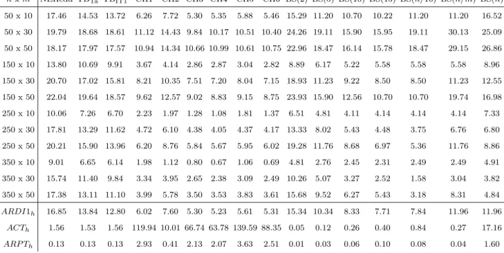
The computational results of the constructive heuristics are shown in Table 2, and in Figure
4. Table 2 shows the results of the ARDI1h for each heuristic h grouped by n and m. The
average results in terms ofACTh,ARP Th, and ARDI1h are shown in the last three rows. The
dominance of each heuristic can be graphically seen in Figure 4 (X-axis and Y-axis indicate the
ARP Th andARDI1h of each heuristich).
The results show that the BS(2), BS(5), BS(10), BS(n/10), and BS(15) algorithms are
ef-ficient for the problem (see red line in Figure 4). To statistically support it (i.e. to discard that they are not statistically better), we perform a non-parametric Wilcoxon signed-rank test
for each one of the following hypotheses: BS(5)=BS(n/m); BS(15)=NEHedd; BS(15)=TBTa;
and BS(15)=TBIT1, where each efficient beam search algorithm has been compared against the
closest heuristic. Thep-value found for each one was 0.000 rejecting each one of the previous
hy-potheses. In addition, several of the proposed beam search algorithms, BS(5), BS(10), BS(n/10),
and BS(15), clearly outpeform the NEHedd and TBIT1 heuristics both in terms of ARDI1 and
ARP T (or ACT). Note that, as stated in Section 1, both heuristics are the key heuristics for
the problem under consideration (the NEHedd heuristic is used as initial solution for most of the algorithms developed for the problem). The excellent performance of the proposed beam search heuristic probably lies in the reduction of the complexity of the evaluation. The complexity of
evaluating a full sequence in theF m|prmu|P
Tj problem is O(nm), while in the proposed
algo-rithm it is onlyO(m) since the jobs are inserted, one by one, at the end of a partial sequence. By
reducing the complexity of this evaluation, the algorithm can evaluate much more sequences in the same CPU time. Regarding the six proposals by Li et al. (2015), which also use the NEHedd as initial solution, they perform better than each other one in terms of quality of the solution
(ARDI1) but requiring much higher CPU times.
nxm NEHedd TBTa TBIT1 CH1 CH2 CH3 CH4 CH5 CH6 BS(2) BS(5) BS(10) BS(15) BS(n/10) BS(n/m) BS(n) 50 x 10 17.46 14.53 13.72 6.26 7.72 5.30 5.35 5.88 5.46 15.29 11.20 10.70 10.22 11.20 11.20 16.52 50 x 30 19.79 18.68 18.61 11.12 14.43 9.84 10.17 10.51 10.40 24.26 19.11 15.90 15.95 19.11 30.13 25.09 50 x 50 18.17 17.97 17.57 10.94 14.34 10.66 10.99 10.61 10.75 22.96 18.47 16.14 15.78 18.47 29.15 26.86 150 x 10 13.80 10.69 9.91 3.67 4.14 2.86 2.87 3.04 2.82 8.89 6.17 5.22 5.58 5.58 5.58 8.96 150 x 30 20.70 17.02 15.81 8.21 10.35 7.51 7.20 8.04 7.15 18.93 11.23 9.22 8.50 8.50 11.23 12.55 150 x 50 22.04 19.64 18.57 9.62 12.57 9.02 8.83 9.15 8.75 23.93 15.90 12.56 10.70 10.70 19.74 16.98 250 x 10 10.06 7.26 6.70 2.23 1.97 1.28 1.08 1.81 1.37 6.51 4.81 4.11 4.14 4.14 4.14 7.33 250 x 30 17.81 13.29 11.62 4.72 6.10 4.38 4.05 4.37 4.17 13.33 8.02 5.43 4.48 3.75 6.76 6.80 250 x 50 20.21 15.90 13.96 6.20 8.76 5.84 5.67 5.95 6.02 19.28 11.76 8.68 6.97 5.36 11.76 8.86 350 x 10 9.01 6.65 6.14 1.98 1.12 0.80 0.67 1.06 0.69 4.81 2.76 2.45 2.31 2.49 2.49 4.91 350 x 30 15.74 11.40 9.84 3.34 3.95 2.65 2.38 3.09 2.49 10.26 5.07 3.27 2.52 1.58 3.04 3.82 350 x 50 17.38 13.11 11.10 3.99 5.78 3.50 3.53 3.83 3.61 15.68 9.52 6.27 5.43 3.18 8.31 4.84 ARDI1h 16.85 13.84 12.80 6.02 7.60 5.30 5.23 5.61 5.31 15.34 10.34 8.33 7.71 7.84 11.96 11.96 ACTh 1.56 1.53 1.56 119.94 10.01 66.74 63.78 139.59 88.35 0.05 0.12 0.26 0.40 0.84 0.27 17.16 ARP Th 0.13 0.13 0.13 2.93 0.41 2.13 2.07 3.63 2.51 0.01 0.03 0.06 0.10 0.08 0.04 1.60
Table 2: ARDI1h for each constructive heuristics grouped by the number of jobs and
machines in each factory. Last three files represent the average results ofARDI1h,ACTh,
Figure 4: ARDI1 versus ARPT for the constructive heuristics
4.6
Metaheuristics
The re-coded algorithms (KIG, TSM63, EA, GAPR, and HA) and our proposals (IARI, IAGI,
IARGS, IAGGS, IARAS, IAGI_ALS, IAILS_GI, and IAGI_ILS) have been run under three different
stopping criteria, i.e. time equals to 60·n·m, 90·n·m, and 120·n·m. The computational results
for these three stopping criteria are shown, grouped by the different levels of each parameter, in Tables 3, 4, and 5, respectively. These results show the good performance of GAPR against the
HA metaheuristic (see hypothesis H1 in Table 6). Regarding the comparison between the last
metaheuristics developed for the problem (i.e. KIG, TSM63, and EA), the KIG metaheuristic
clearly outperforms the other two for the three stopping criteria (hypothesis H2). Regarding our
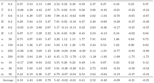
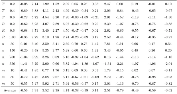
proposals, the following conclusions can be obtained:
1. The random adjacent swap is the best perturbation among our eight proposals, for all time
2. In addition, the IARASis efficient and outperforms each other metaheuristic for the problem
(hypothesis H4).
3. The iterated algorithm based on greedy general swap (IAGGS) performs worst than each
other perturbation method (hypothesis H5).
4. Similarly as in theF m|prmu|Cmax (Dubois-Lacoste et al., 2017), the greedy insertion plus
local search insertion(IAILS_GI) outperforms the greedy insertion (hypothesis H6).
5. The random and greedy insertions (IARI and IAGI, respectively) perform very similar
(hypothesis H7).
To justify each previous conclusion, the following hypotheses are checked for statistical
evi-dence: GAPR=HA (H1);KIG=EA (H2); IAGGS=IAILS_GI(H3);IARAS=KIG (H4); IARAS=IAGI_ILS
(H5); IAGI_ILS=IAGI (H6); and IARI=IAGI (H7). Results are shown in Table 6 for stopping
cri-terion 60·n·m (the same statistical evidences have been found for the other parameters). The
last two columns show the results obtained using Holm’s procedure (see e.g. Pan et al., 2008 and Fernandez-Viagas and Framinan, 2015b for related studies). No statistical evidence has been found only for the hypothesis that the random insertion outperforms the greedy insertion.
In addition, it is worth highlighting that the excellent performance of IARAS probably lies in
performing several small variations in the sequence to decrease the number of “bad” solutions evaluated. The perturbation phase of this iterated algorithm is performed over a sequence which is a local optimum, therefore this sequence is presumably “good” and introducing a high number of changes in this sequence seems to produce, in many cases, sequences that are worse than the initial, but that have to computed, thus wasting CPU effort. Similar results have been found for example both in Rad et al. (2009) and Fernandez-Viagas and Framinan (2015d), which could lead to similar conclusions.
Parameter KIG TSM63 EA GAPR HA IARI IAGI IARGS IAGGS IARAS IAGI_ALS IAILS_GI IAGI_ILS T 0.2 0.27 2.53 2.13 1.69 2.52 0.32 0.49 0.59 2.47 0.27 0.43 0.25 0.37 T 0.4 -0.08 4.39 4.42 2.87 5.75 0.02 0.10 0.56 3.08 -0.43 -0.01 -0.23 -0.24 T 0.6 0.13 6.38 5.07 3.80 7.98 -0.41 -0.62 0.09 2.02 -1.04 -0.70 -0.65 -0.87 R 0.2 0.29 5.94 4.53 3.47 7.91 0.02 -0.16 0.47 2.40 -0.60 -0.28 -0.37 -0.40 R 0.6 -0.05 4.19 3.80 2.67 5.17 -0.14 -0.13 0.32 2.63 -0.46 -0.17 -0.25 -0.37 R 1.0 0.07 3.17 3.29 2.22 3.16 0.05 0.26 0.45 2.53 -0.13 0.16 -0.02 0.04 n 50 0.75 3.97 3.85 5.47 3.20 1.12 1.15 1.77 7.81 0.81 1.06 0.83 0.75 n 150 0.43 5.36 5.47 2.81 5.94 1.19 1.20 1.70 3.43 0.53 1.02 0.90 0.82 n 250 -0.26 4.56 3.69 1.43 6.08 -0.68 -0.68 -0.29 0.14 -1.01 -0.77 -0.83 -0.80 n 350 -0.50 3.84 2.49 1.43 6.45 -1.72 -1.70 -1.53 -1.28 -1.93 -1.69 -1.75 -1.75 m 10 -0.17 2.08 0.94 2.02 3.55 0.26 0.22 0.49 1.81 0.07 0.23 0.23 0.12 m 30 0.05 5.02 4.33 3.07 5.91 -0.26 -0.20 0.21 2.72 -0.63 -0.33 -0.50 -0.52 m 50 0.43 6.19 6.36 3.27 6.79 -0.07 -0.04 0.53 3.04 -0.64 -0.19 -0.37 -0.34 Average 0.10 4.43 3.88 2.79 5.42 -0.02 -0.01 0.41 2.52 -0.40 -0.09 -0.21 -0.25
Table 3: AverageRDI1h of each metaheuristic for stopping criterion 60·n·mms grouped
by the values of the parameters.
Parameter KIG TSM63 EA GAPR HA IARI IAGI IARGS IAGGS IARAS IAGI_ALS IAILS_GI IAGI_ILS T 0.2 0.06 2.32 2.00 1.59 2.23 0.16 0.34 0.46 2.47 0.11 0.28 0.07 0.20 T 0.4 -0.58 4.06 4.20 2.58 5.24 -0.24 -0.15 0.39 3.07 -0.70 -0.30 -0.51 -0.50 T 0.6 -0.39 6.02 4.76 3.40 7.48 -0.64 -0.92 -0.06 2.01 -1.31 -0.98 -0.95 -1.12 R 0.2 -0.28 5.53 4.25 3.12 7.31 -0.23 -0.43 0.31 2.40 -0.88 -0.56 -0.62 -0.71 R 0.6 -0.47 3.90 3.55 2.40 4.72 -0.34 -0.35 0.19 2.63 -0.69 -0.39 -0.54 -0.56 R 1.00 -0.16 2.96 3.16 2.05 2.93 -0.15 0.05 0.30 2.52 -0.33 -0.04 -0.23 -0.15 n 50 0.52 3.67 3.69 5.41 2.85 0.90 0.91 1.59 7.81 0.65 0.80 0.58 0.62 n 150 0.06 4.85 5.32 2.77 5.50 0.87 0.83 1.48 3.43 0.18 0.70 0.47 0.44 n 250 -0.73 4.20 3.39 0.94 5.44 -0.86 -0.89 -0.40 0.13 -1.27 -0.97 -1.01 -1.03 n 350 -1.06 3.81 2.22 0.97 6.16 -1.87 -1.82 -1.61 -1.30 -2.09 -1.85 -1.90 -1.94 m 10 -0.33 1.95 0.84 1.83 3.29 0.14 0.09 0.42 1.79 -0.07 0.11 0.14 -0.03 m 30 -0.41 4.68 4.05 2.80 5.44 -0.48 -0.44 0.03 2.72 -0.88 -0.57 -0.82 -0.78 m 50 -0.17 5.76 6.07 2.94 6.22 -0.38 -0.38 0.33 3.04 -0.95 -0.53 -0.71 -0.62 Average -0.30 4.13 3.65 2.52 4.99 -0.24 -0.24 0.26 2.52 -0.63 -0.33 -0.47 -0.47
Table 4: AverageRDI1h of each metaheuristic for stopping criterion 90·n·mms grouped
Parameter KIG TSM63 EA GAPR HA IARI IAGI IARGS IAGGS IARAS IAGI_ALS IAILS_GI IAGI_ILS T 0.2 -0.08 2.14 1.92 1.52 2.02 0.05 0.25 0.38 2.47 0.00 0.19 -0.01 0.10 T 0.4 -0.89 3.88 4.11 2.42 4.99 -0.39 -0.34 0.24 3.06 -0.84 -0.46 -0.65 -0.67 T 0.6 -0.72 5.72 4.54 3.20 7.20 -0.80 -1.09 -0.21 2.01 -1.52 -1.19 -1.11 -1.30 R 0.2 -0.62 5.25 4.07 2.89 6.97 -0.39 -0.62 0.20 2.39 -1.07 -0.75 -0.75 -0.88 R 0.6 -0.68 3.71 3.40 2.27 4.50 -0.47 -0.47 0.02 2.62 -0.86 -0.55 -0.67 -0.71 R 1.00 -0.38 2.79 3.10 1.98 2.74 -0.28 -0.09 0.19 2.52 -0.44 -0.17 -0.35 -0.27 n 50 0.40 3.40 3.59 5.41 2.69 0.79 0.76 1.42 7.81 0.54 0.66 0.47 0.54 n 150 -0.20 4.48 5.25 2.77 5.28 0.60 0.60 1.32 3.43 -0.05 0.48 0.26 0.20 n 250 -1.04 3.99 3.26 0.69 5.16 -0.97 -1.04 -0.52 0.13 -1.44 -1.13 -1.14 -1.18 n 350 -1.41 3.79 2.00 0.66 5.82 -1.94 -1.89 -1.67 -1.31 -2.21 -1.97 -1.96 -2.04 m 10 -0.41 1.85 0.77 1.76 3.13 0.09 0.00 0.33 1.78 -0.15 0.02 0.07 -0.11 m 30 -0.72 4.42 3.88 2.67 5.17 -0.67 -0.61 -0.09 2.72 -1.06 -0.78 -0.98 -0.93 m 50 -0.55 5.47 5.92 2.71 5.91 -0.56 -0.57 0.17 3.03 -1.16 -0.70 -0.87 -0.82 Average -0.56 3.91 3.52 2.38 4.74 -0.38 -0.39 0.14 2.51 -0.79 -0.49 -0.59 -0.62
Table 5: Average RDI1h of each metaheuristic h for stopping criterion 120·n ·m ms
grouped by the values of the parameters.
Hi Hypothesis p-value Wilcoxon α/(7−i+ 1) Holm’s procedure
H1 GAPR=HA 0.000 R 0.0071 R
H2 KIG=EA 0.000 R 0.0083 R
H3 IARAS=IAGI_ILS 0.000 R 0.0100 R
H4 IARAS=KIG 0.000 R 0.0125 R
H5 IAGGS=IARGS 0.000 0.0167
H6 IAILS_GI=IAGI 0.000 0.0250
H7 IARI=IAGI 0.939 0.0500
Table 6: Holm’s procedure.
5
Conclusions
In this paper we have proposed two different sets of algorithms to solve the permutation flow shop scheduling problem to minimise the total tardiness. Firstly, we have proposed a set of
beam-search-based heuristics varying the size of their population. These are fast heuristics that construct solutions by adding jobs at the end of several partial sequences constructed in parallel. In addition, this set uses properties of the problem both to estimate the performance of each partial sequence and to be able to compare sequences with different jobs. Secondly, we have proposed several simple iterated-greedy-based algorithms with several types of destruction-construction phases. The methods developed to perturb the solutions are based on insertion, general swap, adjacent swap, and partial local searches.
Our proposals have been compared with the state-of-the-art algorithms of the problem under study in a well-known benchmark testbed. More specifically, a total of 14 algorithms have been reimplemented and compared with our proposals (a set of beam search algorithms varying the size of the population, and eight different iterated algorithms). Regarding constructive heuristics, the results show that BS(15) clearly outperforms the NEHedd in terms of quality of solutions
and computational effort. In addition, the proposed heuristics BS(2), BS(5), BS(10), BS(n/10),
and BS(15) are efficient heuristics for the problem. Regarding the computational evaluation
of metaheuristics, the iterated algorithm with a simple random adjacent swap (IARAS) clearly
outperforms the other seven simple and complex perturbation methods of the iterated algorithm, and statistically outperforms each other existing metaheuristic for the problem under study.
Due to the excellent performance of the original iterated greedy in different scheduling prob-lems, it is noteworthy to mention that the conclusions obtained by applying the simple random adjacent swap, such as the destruction-construction phase of the proposed iterated algorithm, could probably be extended for future iterated-greedy-based algorithms developed for either the problem under consideration, or for related scheduling problems.
Acknowledgements
This research has been funded by the Spanish Ministry of Science and Innovation, under projects “ADDRESS” with reference DPI2013-44461-P and “PROMISE” with reference DPI2016-80750-P.
References
Cura, T. (2015). An evolutionary algorithm for the permutation flowshop scheduling problem
with total tardiness criterion. International Journal of Operational Research, 22(3):366–384.
Dong, X., Huang, H., and Chen, P. (2009). An iterated local search algorithm for the permutation
flowshop problem with total flowtime criterion.Computers & Operations Research, 36(5):1664–
1669.
Du, J. and Leung, J. (1990). Minimizing total tardiness on one machine is np-hard.Mathematics
of Operations Research, 15(3):483–495.
Dubois-Lacoste, J., Pagnozzi, F., and Stützle, T. (2017). An iterated greedy algorithm with
optimization of partial solutions for the makespan permutation flowshop problem. Computers
and Operations Research, 81:160–166.
Fernandez-Viagas, V., Dios, M., and Framinan, J. (2016a). Efficient constructive and composite
heuristics for the permutation flowshop to minimise total earliness and tardiness. Computers
and Operations Research, 75:38–48.
Fernandez-Viagas, V. and Framinan, J. (2015a). A bounded-search iterated greedy algorithm for
the distributed permutation flowshop scheduling problem.International Journal of Production
Research, 53(4):1111–1123.
Fernandez-Viagas, V. and Framinan, J. (2015b). Efficient non-population-based algorithms for the permutation flowshop scheduling problem with makespan minimisation subject to a
max-imum tardiness. Computers & Operations Research, 64(0):86 – 96.
Fernandez-Viagas, V. and Framinan, J. (2015c). A new set of high-performing heuristics to
minimise flowtime in permutation flowshops. Computers & Operations Research, 53:68–80.
Fernandez-Viagas, V. and Framinan, J. (2015d). NEH-based heuristics for the permutation
flowshop scheduling problem to minimise total tardiness. Computers & Operations Research,
60:27–36.
Fernandez-Viagas, V. and Framinan, J. (2017). A beam-search-based constructive heuristic for
the pfsp to minimise total flowtime. Computers and Operations Research, 81:167–177.
Fernandez-Viagas, V. and Framinan, J. M. (2014). On insertion tie-breaking rules in heuristics
for the permutation flowshop scheduling problem. Computers & Operations Research, 45(0):60
– 67.
Fernandez-Viagas, V., Leisten, R., and Framinan, J. (2016b). A computational evaluation of constructive and improvement heuristics for the blocking flow shop to minimise total flowtime.
Expert Systems with Applications, 61:290–301.
Fernandez-Viagas, V., Ruiz, R., and Framinan, J. (2017). A new vision of approximate meth-ods for the permutation flowshop to minimise makespan: State-of-the-art and computational
evaluation. European Journal of Operational Research, 257(3):707–721.
Framinan, J. and Leisten, R. (2008). Total tardiness minimization in permutation flow shops:
A simple approach based on a variable greedy algorithm. International Journal of Production
Research, 46(22):6479–6498.
Hasija, S. and Rajendran, C. (2004). Scheduling in flowshops to minimize total tardiness of jobs.
International Journal of Production Research, 42(11):2289–2301.
permutation flowshops. Computers and Industrial Engineering, 98:300–307.
Kim, Y.-D. (1993). Heuristics for flowshop scheduling problems minimizing mean tardiness.
Journal of the Operational Research Society, 44(1):19–28.
Kim, Y.-D., Lim, H.-G., and Park, M.-W. (1996). Search heuristics for a flowshop
schedul-ing problem in a printed circuit board assembly process. European Journal of Operational
Research, 91(1):124–143.
Li, X., Chen, L., Xu, H., and Gupta, J. (2015). Trajectory scheduling methods for minimizing
total tardiness in a flowshop. Operations Research Perspectives, 2:13–23.
Li, X., Wang, Q., and Wu, C. (2009). Efficient composite heuristics for total flowtime
minimiza-tion in permutaminimiza-tion flow shops. OMEGA, The International Journal of Management Science,
37(1):155–164.
Liu, J. and Reeves, C. (2001). Constructive and composite heuristic solutions to the P||Pc
i
scheduling problem. European Journal of Operational Research, 132:439–452.
Naderi, B. and Ruiz, R. (2010). The distributed permutation flowshop scheduling problem.
Computers & Operations Research, 37(4):754–768.
Nawaz, M., Enscore Jr., E., and Ham, I. (1983). A heuristic algorithm for the m-machine, n-job
flow-shop sequencing problem. OMEGA, The International Journal of Management Science,
11(1):91–95.
Pan, Q.-K., Gao, L., Li, X.-Y., and Gao, K.-Z. (2017). Effective metaheuristics for scheduling a
hybrid flowshop with sequence-dependent setup times.Applied Mathematics and Computation,
303:89–112.
Pan, Q.-K. and Ruiz, R. (2013). A comprehensive review and evaluation of permutation flowshop
heuristics to minimize flowtime. Computers & Operations Research, 40(1):117–128.
Pan, Q.-K. and Ruiz, R. (2014). An effective iterated greedy algorithm for the mixed no-idle
permutation flowshop scheduling problem. Omega (United Kingdom), 44:41–50.
Pan, Q.-K., Tasgetiren, M., and Liang, Y.-C. (2008). A discrete differential evolution algorithm
for the permutation flowshop scheduling problem. Computers and Industrial Engineering,
55(4):795–816.
Panwalkar, S., Smith, M., and Seidmann, A. (1982). Common due date assignment to minimize
total penalty for the one machine scheduling problem. Operations Research, 30(2):391–399.
Parthasarathy, S. and Rajendran, C. (1997). A simulated annealing heuristic for scheduling to minimize mean weighted tardiness in a flowshop with sequence-dependent setup times of
jobs-a case study. Production Planning and Control, 8(5):475–483.
Parthasarathy, S. and Rajendran, C. (1998). Scheduling to minimize mean tardiness and weighted
mean tardiness in flowshop and flowline-based manufacturing cell. Computers and Industrial
Engineering, 34(2-4):531–546.
Pinedo, M. (1995). Scheduling: Theory, Algorithms and Systems. Prentice Hall.
Potts, C. and Van Wassenhove, L. (1982). A decomposition algorithm for the single machine
total tardiness problem. Operations Research Letters, 1(5):177–181.
Rad, S. F., Ruiz, R., and Boroojerdian, N. (2009). New high performing heuristics for minimizing
makespan in permutation flowshops. OMEGA, The International Journal of Management