Functional characterization and annotation of trait-associated genomic regions by transcriptome analysis

(1)

Functional characterization

and annotation of

trait-associated genomic regions

by transcriptome analysis

Dissertation zur

Erlangung des akademischen Grades Doktor-Ingenieur (Dr.-Ing.) Promotionsgebiet Bioinformatik Fakultät für Informatik und Elektrotechnik

Universität Rostock

vorgelegt von

Yang Du, geboren am03. Feburar 1983in Tianjin

aus Rostock

(2)

Prof. Dr.-ing. Thomas Kirste (MMIS, Universität Rostock)

Prof. Dr. rer. nat. Klaus Wimmers (Leibniz-Institut für Nutztierbiologie, Dummer-storf)

Prof. Dr. rer. nat. Georg Füllen (IBIMA, Universitätsmedizin Rostock) Prof. Dr. rer. nat. Mario Stanke (MNF, Universität Greifswald)

Datum der Einreichung: 16. Juni2014

(3)

(4)

I would like to first express my very great appreciation to my supervisor at FBN, Prof. Klaus Wimmers, for his generosity, support and patience throughout my work, for which I will always be grateful. With my deepest gratitude, I would also like to thank Prof. Thomas Kirsteand Prof. Georg Füllen, for accepting me and supporting my work, and their insightful comments and useful critiques of this research work. Without their guidance and encouragement, I would not be able to finish this dissertation.

My grateful thanks are also extended to Dr. Siriluck Ponsuksili, Dr. Eduard Murani and Dr. Nares Trakooljul, for their valuable advices and resultful discussions. It has been a great pleasure and learning opportunity to work with them in those past and on-going projects.

I am particularly grateful for the lab assistance given by Ms Hannelore Tychsen during the tiling array experiments. Despite the occasional language barrier, it has been a truly rewarding experience to work with her, and to see for oneself how experiments are done in real world.

I would like to offer my special thanks to Dr. Ronald Brunner, Frieder Hadlich, and also Peter Havemann from the IT department, for their excellent technical support with computational servers and web hosting.

I would also like to extend my thanks to many people from the university, for their openness to help, and for their suggestions and comments in many stages of my thesis preparation. It was truely uneasy for an external PhD student to walk though these process alone.

I wish to thank all my colleagues and friends at FBN, Au, Philipp, Ta, Wiebke, Tum, Milan..., it is impossible to name you all, for those German / Biology101s, for helping me settle down and get through those tough transitions, for those laughters we shared and those fun get-togethers. Thank you all who had been kind to me and made my stay in Germany both scientifically and socially rewarding.

Last but not least, I want to specially thank my family and friends, here and at home, for their love, continuous encouragement and support during the time that I was en-gaged in this study.

(5)

Abstract

Functional genomics is the subject of studying biological data recorded in the com-plete state of a genomic system using high-throughput techniques, to describe the func-tion of DNA and its interacfunc-tions with intermediate RNA transcripts and funcfunc-tional pro-tein products. One of the most crucial issues to deal with in genomics is the ambiguity arising from sequence homology. Duplicated DNA sequences of variable length com-monly exist in most organisms, which impose a great challenge on the technologies used in genome research. As the two flagship high-throughput techniques used to character-ize genomes and trnascriptomes and to quantify the level of various biological activities and redundancy, tiling array and next-generation sequencing both require careful han-dling of non-uniquely mapped features to ensure their accuracies. Thus many works have been done in the field of array probe design and in mapping sequencing reads back to reference or inde novo genome assembly. According to the recent result from the international collaboration effort, The ENCODE project, 80 percent of the human genome are either transcribed or biochemically functional, a number much higher than the known protein coding segments scientists used to believe even in2003, when the human genome was fully sequenced. As a consequence of the growing availability of new high-throughput techniques, many of such novel functional fragments need to be identified and further functionally characterized. In this work, two novel imple-mentations have been presented, which could assist in the design and data analysis of high-throughput genomic experiments. An efficient and flexible tiling probe selection pipeline utilizing the penalized uniqueness score has been implemented, which could be employed in the design of various types and scales of genome tiling task, with high coverage and resolution, while giving more control of the expected hybridization effi-ciency. A novel hidden semi-Markov model (HSMM) implementation is made available within the Bioconductor project, which provides a unified interface for segmenting ge-nomic data in a wide range of research subjects. It was designed specifically for gege-nomic data analysis, with flexible distributional assumption and optional prior learning using annotation or previous studies. The usages and performance of the two novel tools have been illustrated and evaluated using simulation and published datasets. Moreover, through an integrative and detailed case study, in which genome regions previously show to exhibit quantitative trait loci (QTL) should be characterized in terms of en-coding differentially expressed genes, the two implementations have been utilized. The penalized uniqueness score was used to design1M feature tiling arrays that covered a18 Mb region of the porcine genome at a coverage of49%. The HSMM was applied on the data from hybridization experiments of divergent animals enabled detecting candidate genes with trait-dependent expression.

(6)

(7)

Zusammenfassung

Die funktionale Genomik verfolgt als Ziele die allumfassende Auswertung biolo-gischer Daten eines genomischen Systems mittels Hochdurchsatz-Technologien sowie die funktionale Charakterisierung der DNA und ihrer Wechselwirkungen mit RNA-Transkripten und funktionalen Proteinprodukten. Eine der größten Hürden in der Genomik stellt hierbei die Uneindeutigkeit durch Sequenzhomologien dar. Redun-dante DNA-Sequenzen variabler Länge existieren in vielen Organismen und bilden eine enorme Herausforderung an die Technologien in der genomischen Forschung. Sogenan-nte tiling arrays und Next-Generation-Sequenzierung sind Hochdurchsatz-Technologien, deren Daten eine sorgfältige Überprüfung und Bearbeitung hinsichtlich mehrfach kartierter Sequenzen zur Wahrung ihrer Präzision. Folglich wurden bereits viele Anstrengungen unternommen zum Erstellen von Arrayproben und beim Assemblieren von Fragmenten von Sequenzen gegen Referenzgenome bzw. bei der De-novo Assemblierung. Neueste Ergebnisse aus dem ENCODE Projekt, einer internationaler Verbundarbeit, belegen, dass 80 Prozent des menschlichen Genoms entweder transkribiert oder biochemisch funktional sind, also deutlich mehr als Wissenschaftler noch2003bei der Vervollständi-gung des Humangenoms angenommen haben. Als Konsequenz der stetig wachsenden Verfügbarkeit neuer Hochdurchsatz-Technologien müssen viele der neu gefundenen funktionalen Fragmente identifiziert und weiter funktional charakterisiert werden. In dieser Arbeit werden zwei neuartige Implementierungen präsentiert, die im Design und in der Datenanalyse von genomischen Hochdurchsatz-Experiment hilfreich sein können. Die erste Implementierung bildet eine effiziente und flexible Auswahl-Pipeline für tiling Proben basierend auf einem Eindeutigkeitsmaßmit einer Maluswertung (pe-nalized uniqueness score), welches in vielfältigen Formen und Anwendungen für tiling Sonden ein Sondendesign mit einer hohe Abdeckungs- und Auflösungsrate ermöglicht und zudem mehr Kontrolle an erwarteter Hybridisierungeffizienz verspricht. Als zweite Implementierung wurde ein neuartiges Hidden-Semi-Markov-Modell (HSMM) im Bio-conductor Projekt verfügbar gemacht, welches speziell für die genomische Datenanalyse mit flexibler Verteilungsannahme und optionalen Vorkenntnissen in Form von Annota-tionen oder Vorstudien die Segmentierung genomischer Daten in einer weiten Band-breite von Forschungsvorhaben durch ihre einheitliche Schnittstelle unterstützt. An-wendbarkeit sowie Leistungsfähigkeit beider Programme sind mit Hilfe von simulierten und publizierten Daten dargestellt. In einer integrativen und detaillierten Fallstudie am Beispiel von Zuchttieren, bei dem zuvor identifizierte QTL (quantitativ trait loci) Regio-nen hinsichtlich differentiell exprimierter Gene charakterisiert werden sollten, wurden beide Implementationen angewendet Der penalized uniqueness score wurde genutzt um einen tiling array mit1mio Element abzuleiten der eine18mb große region des

(8)

porci-einem Hybridisierungsexperiment mit divergenten Tieren eingesetzt und ermöglichte die Identifizierung von merkmalsabhängig exprimierten Kandidatengene.

(9)

Acronym

A Adenine

aCGH Microarray-based comparative ge-nomic hybridization

AUC area under the curve

BAC bacterial artificial chromosome

BLAST Basic Local Alignment Search Tool

BLAT BLAST-Like Alignment Tool

BP Biological Process

BWT Burrows—Wheeler transform

C Cytosine

CBS Circular Binary Segmentation

CC Cellular Component

CDF cumulative distribution function

cDNA complementary deoxyribonucleic acid (DNA)

CNV copy number variation CT threshold cycle

ChIP chromatin immunoprecipitation

DBN dynamic Bayesian network

DEPs differentially expressed probes

DEGs differentially expressed genes

DMRs differentially methylated regions

DNase deoxyribonuclease

DNA deoxyribonucleic acid

EM expectation—maximization

FDR false discovery rate

FPR false positive rate

FM-index Full-text index in Minute space

G Guanine

GC Guanine-Cytosine

GEO Gene Expression Omnibus

GO Gene Ontology

GWAS Genome Wide Association Studies

HMM Hidden Markov Model

HSMM Hidden semi-Markov Model

IPA Ingenuity pathway analysis

LINEs long interspersed nuclear elements

LOH loss of heterozygosity

LTR long terminal repeat

MAE mean absolute error

MCMC Markov chain Monte Carlo

MDS multidimensional scaling

MeDIP methylated DNA immunoprecipi-tation

MF Molecular Function

(10)

Information

NGS Next-generation sequencing

ORF open reading frame

QC quality control

qPCR quantitative polymerase chain reac-tion

RLE run-length encoding

RMSE rooted mean squared error

SINEs short interspersed nuclear elements

SNP single-nucleotide polymorphism

SNR signal-to-noise ratio

T Thymine

Tm melting temperature

TPR true positive rate

(11)

List of Figures

1.1. A schematic illustration of microarray . . . 2

1.2. Tiling array probe layouts . . . 3

1.3. Microarray data analysis flow . . . 4

1.4. Comparison of Sanger sequencing and NGS work flow . . . 6

2.1. Summary of repetitive DNA sequences in the human genome . . . 14

2.2. Schematic diagram of low MUS coverage and long MUS . . . 19

2.3. Back-to-back box-plot of uniqueness score distributions . . . 21

2.4. ROC curves of uniqueness scores comparison . . . 24

2.5. Palindromic content and uniqueness scores of Agilent ChIP-on-Chip Set 28 2.6. Palindromic content and uniqueness scores of experimental data . . . 29

2.7. Schematic of HMM parametrization . . . 33

2.8. Example of simulated data and estimated segments . . . 42

2.9. ROC curves of segmentation model performance comparison . . . 43

2.10. Copy number profile of Corriell data . . . 50

2.11. Estimated sojourn densities . . . 54

2.12. Novel transcript detection in RNA-seq data . . . 55

2.13. Detected differentially methylated regions . . . 59

3.1. Correlation between Affymetrix GeneChip and customary tiling array . . 68

3.2. Venn diagram of detected DEGs and DEPs regions . . . 69

3.3. Schematic illustration of DEPs definition . . . 70

3.4. Histogram and density plot of the pseudo array probe signal . . . 77

3.5. Correlation of the tiling array and the pseudo array . . . 79

3.6. Example splicing events . . . 81

3.7. MDS plot of mRNA-seq samples . . . 82

3.8. mRNA-seq profiles of intronic DEPs regions . . . 91

3.9. mRNA-seq profiles of exonic DEPs regions . . . 92

3.10. mRNA-seq profiles of DEPs regions with HSMM prediction . . . 93

(14)

(15)

List of Tables

2.1. Nearest-Neighbor parameters for DNA/DNA duplex . . . 12

2.2. Summary of Agilent ChIP-on-Chip Set probe properties . . . 20

2.3. Example of problematic60-mer probes from Agilent ChIP-on-Chip Set . 22 2.4. Parameters of tiling probe selection algorithm . . . 23

2.5. Summary of experiments from ArrayExpress . . . 25

2.6. Design summary and coverage comparison . . . 27

2.7. List of segmentation algorithms compared . . . 40

2.8. Area under the ROC curves of simulation data1. . . 44

2.9. Area under the ROC curves of simulation data2. . . 45

2.10. Processing time and error estimates of the compared models . . . 46

3.1. Populations and Phenotypes . . . 62

3.2. Experimental panel of tiling array samples . . . 63

3.3. Candidate genomic regions to be tiled on the array . . . 65

3.4. Correlation between Affymetrix GeneChip and customary tiling array . . 67

3.5. Common genes overlapped with DEPs regions . . . 71

3.6. Common DEPs genes to GO MF test for over-representation . . . 73

3.7. Common DEPs genes to GO BP test for over-representation . . . 74

3.8. Ingenuity Canonical Pathways of common DEPs genes . . . 75

3.9. Experimental panel of mRNA-seq samples . . . 76

3.10. Distribution of the sum of pseudo array probe signals across samples . . 77

3.11. Correlation of the tiling array and the pseudo array . . . 78

3.12. Significant DEGs and common DEPs genes in mRNA-seq . . . 84

3.13. Commonly detected DEPs regions . . . 88

3.14. Correlation of qPCR expression with tiling array and pseudo array . . . . 89

(16)

(17)

CHAPTER

1

Introduction

As an experimental science, biology used to be a time and labor intensive research subject. While in the last few decades, thanks to laboratory automation and high-throughput technologies, a new branch of contemporary genetics research, genomics, has been created, which is the studying of structure and function of the complete set of DNA from an organism. Transcriptome profiling is one of the first steps to understand complex biological processes, which helps us to move forward from genomic DNA sequences, the most basic genetic materials, to functional proteins. As the two most widely adopted high through-put technologies to survey transcriptome, genome tiling array and next-generation sequencing (NGS) give us the opportunity to unbiasedly cap-ture the transcription activity across genomic regions. In this chapter, we will make brief introduction of these two experimental technologies, and present the key objectives of this dissertation.

1.1. Microarray

A DNA microarray or DNA chip is a highly compact assay of microscopic spots with se-lected specific DNA sequence, the probe, deposited or attached to a solid surface which normally taking the form of quartz slide or plastic chip. Alternative form also includes using immobilized microscopic beads without a solid platform. After hybridization, the signal intensity of the probe is then determined optically by the amount of fluorescently labeled target sample binded to the probe sequence via laser agitation. A schematic illus-tration of microarray is shown in Figure1.11. The application of microarry dates back to 1980s, when some hundreds or thousands of complementary DNA (cDNA) sequences

1

(18)

were spotted onto filter paper to study tissue or treatment specific gene expressions [1;2;3]. The later introduction of computer assisted image scanning and quantification, together with development of robotic spotting and in-situ oligonucleotide synthesizing eventually set the standards of modern miniaturized microarray [4].

Figure1.1.:A schematic illustration of probe hybridization mechanism of microarray.

Various types of microarray are commonly used in genetic research and medical diag-nosis. Gene expression chip, the most popular microarray form, is highly cost efficient to measure expression levels of known genes and transcripts genome-wide. Another fre-quently adopted microarray is the single-nucleotide polymorphism (SNP) array, which is used to survey nucleotide variation in genomic DNA. SNP array is commonly applied in Genome Wide Association Studies (GWAS) of common and complex diseases. Also SNP could serve as both indicators of chromosome copy number and genotype maker, thus enabling the usage of SNP array to study copy number variation (CNV) and loss of heterozygosity (LOH) in cancer.

As another unique variety of high throughout microarray, genome tiling array targets not only known transcripts that are dispersed across the genome, but intensively covers all known contiguous regions on the genome with overlapping or evenly-spaced probes (See Figure1.22), thus being more unbiased than common gene expression arrays. Other than transcriptome profiling, tiling array also aids in discovering sites of DNA/protein interaction (chromatin immunoprecipitation (ChIP)-chip), of DNA methylation (methy-lated DNA immunoprecipitation (MeDIP)-chip) and of sensitivity to deoxyribonucle-ase (DNdeoxyribonucle-ase)-chip) and Microarray-bdeoxyribonucle-ased comparative genomic hybridization (aCGH). Besides whole genome tiling array, region specific tiling also assists in refined

transcrip-2

(19)

1.1. Microarray

Figure1.2.:Common tiling array probe layouts, which could be either overlapping,

end-to-end or with an average spacing between neighbouring probes.

tome profiling of genome regions of interest.

Irrespective of specific microarray types, common work flow (See Figure1.33) of mi-croarray experiment design and data analysis includes statistical power analysis, array quantification, array quality control (QC), statistical analysis and further mining of func-tional genomics data [6].

3

(20)

(21)

1.2. NGS

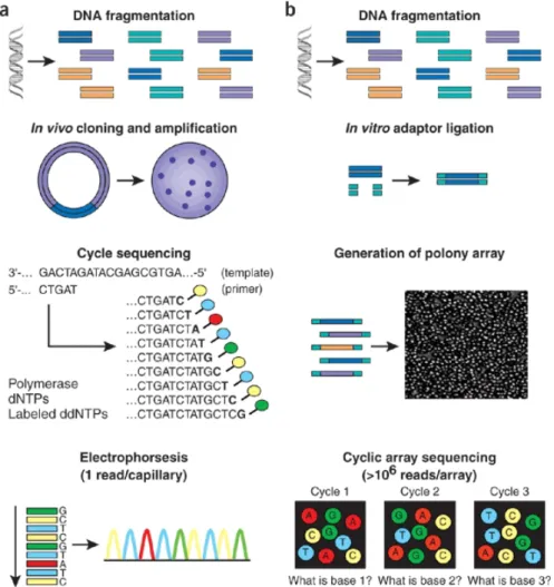
DNA sequencing is the process of sequentially determining the exact order of the four nucleotide bases—Adenine (A), Guanine (G), Cytosine (C), and Thymine (T) in the DNA molecule. To date, the most widely used sequencing method is Sanger sequencing de-veloped by Frederick Sanger and colleagues in 1977. In recent years with advancing technology and lower costs, Next-generation sequencing (NGS) has gained unprece-dented attention in genome research, which has the capability of running hundreds of thousands sequencing operations in parallel (See Figure 1.44 for a simplified compari-son of Sanger sequencing and NGS work flow). With its inherent single-base resolution, NGS achieves higher accuracy in exon boundary mapping and can be used for SNP detection. Furthermore, its unlimited dynamic range enables detection of any subtle changes in gene expressions. Similar to genome tiling array, various types of genomics application can also be addressed by NGS — to quantify mature transcripts and small RNA using mRNA-seq, to survey transcription factor-binding sites with ChIP-seq, to study DNA methylation by MeDIP-seq, and etc [8].

Unlike microarray, for which signals of probes targeting known reference genome sequences can be easily subtracted from image background, the end products of se-quencing experiments are millions of read segments which need to be quantified. The analysis of NGS data is far from mature comparing to microarray data analysis. The alignment of short reads to the reference genome, or de novo assembly of short reads both pose significant challenges to NGS data analysis. Further normalization, visual-ization and statistical modeling of genomic count data are also active fields of ongoing bioinformatics and statistical genetics research.

4

(22)

Figure1.4.:Simplified comparison of Sanger sequencing (a) and NGS (b) work flow. The main differences include the substitution of in vivo cloning with sequencing libraries construction using clonal amplification and the array based parallel cyclic sequencing.

(23)

1.3. Aim of this work

In order to perform scientifically proof research and reveal statistically sensible findings in biology, one of the most basic requirements, the experimental conditions, environ-mental and biological, must be carefully designed and strictly controlled. In addition, a sufficiently large sample of qualified experiment subjects must be available for ma-nipulation. Thus animal models provide an ideal resource for applied agricultural and experimental biology research. Also due to their immense similarities to human, genet-ical and physiologgenet-ical, animal models have been widely used to study human diseases. Functional genomics is the subject of studying biological data recorded in the com-plete state of a genomic system using high-throughput techniques, to describe the func-tion of DNA and its interacfunc-tions with intermediate RNA transcripts and funcfunc-tional pro-tein products. Genome tiling array and next-generation sequencing are the two flagship high-throughput technologies for current functional genomics research.

Unlike gene expression arrays or SNP arrays, high density genome wide tiling arrays are only commercially available for some model organisms, not to mention many other customary tiling arrays of specific purposes. It is also important to note that, due to the well known cross hybridization problem, which haunts microarray technology, and other probe quality issues, successful array based experiment at genome scale requires optimum and proper probe selection method. On the other hand, as the technology progressing, the study of genomics has entered the era of big data. The newly prevailing next-generation sequencing technology has the capability of generating hundreds of gigabytes per run. The accompanying high volume data demands efficient and scalable computational tools to assist in statistical modeling and data visualization.

In this work we will apply custom regional tiling array and next-generation sequenc-ing experiments to identify and functionally characterize traits related genomic re-gions using farm animal model, and contribute to the software development of high-throughput computational biology.

The thesis work presented here is organized as the following,

• Chapter 2: "Methods and models", subdivided into two subsections, surveys and summarizes the common methods and issues involved in tiling array design and genomic segmentation related applications. The development made in the tilling array design using penalized uniqueness score has been published as Yang Du

et al. [9]. The general-purpose genomic segmentation tool implemented has been published inYang Duet al. [10].

(24)

• Chapter3: "Case studies", illustrates the usage of tools developed and presented in the previous chapter through a series of experiments carried out by the re-search group at FBN (Leibniz Institute for Farm Animal Biology, Dummerstorf, Germany).

• Chapter4: "Discussion and Outlooks", further reviews in detail the miscellaneous differences of the proposed methods and models with the existing ones, and dis-cusses related issues in contemporary genomics research. Finally summarizes the works done throughout this dissertation, and discusses further improvements and outlooks in the research fields.

(25)

CHAPTER

2

Methods and Models

In this chapter, I will first review the common methodologies involved in array design, then introduce the concept and usage of penalized uniqueness score in tiling array de-sign. In the second half, the topic will be shifted from experimental design and prepa-ration to statistical modeling and data visualization in genomics. A general-purpose genomic segmentation model will be described and evaluated using simulation and published datasets.

2.1. Custom tiling array design

2.1.1. Common methods and issues

The fundamental bio-chemical principle of microarray technology is the hybridization between two strands of DNA formed by hydrogen bonding of complementary base pairs. Strong and reliable microarray probe signal strength then largely depends on a large number of specific complementary base paring with high sensitivity. Other influ-ential factors contributing to hybridization efficiency are mostly nucleic acid thermody-namics related, like melting temperature (Tm), sequence base compositions, sequence complexity and propensity for secondary structure.

In a successful microarray design, selected probes should have similar hybridization efficiencies under a specified narrow band of temperature, as well as minimal potential for both self-hybridization and cross-hybridization [11]. Further guidelines for the speci-ficity of long oligonucleotides array probe have been discussed in [12], in which the au-thors suggest that candidate probes should exhibit less than75% overall sequence sim-ilarities with non-target sequences and contain no stretch of complementary sequence

(26)

longer than15bases.

However, these selection constraints become much more difficult to satisfy when ap-plied to tiling probes designed for a large genome region [13], and naive method of using a uniform grid is clearly not optimum when considering hybridization efficiency. Among these contributing factors, non-specific binding or cross-hybridization is most problematic, when a non-targeted nucleotide sequence hybridizes to the designed probe. A similar situation with lower specificity also troubles NGS, when short reads need to be either aligned to a reference genome or assembled into contigsde novo[14].

Homogeneity and sensitivity

The melting temperature (Tm), defined as the temperature at which50% of the oligonu-cleotide and its perfect complement are in duplex and the other half are in the random coil state, is essential for the success of stable hybridization, where a narrow band of Tm across all probes is highly desirable [11;13]. It has also been shown that the melting temperature of the probe, among other oligonucleotide properties, might has the most significant impact on hybridization signal intensities [15]. In general, the melting tem-perature is affected by three major factors, oligo concentration, salt concentration and oligo sequence [16]. Common thermodynamics prediction models utilizing only base composition, like GC content or base counts, have been proposed and widely used in practice for short oligonucleotides [17;18;19]. GC content plays a crucial role in probe hybridization, since base pairings between G and C have three hydrogen bonds and are more stable compared to the A / T pairing.

Tm= (#A+#T)×2+ (#G+#C)×4 (2.1)

Tm=64.9+41×(#G+#C−16.4)/(#A+#T+#G+#C) (2.2)

Assuming a standard oligo concentration of 50 nM and pH neutral annealing envi-ronment, Equation (2.1) is valid for sequences shorter than 14 nucleotides [17], while Equation (2.2) is more accurate for sequences longer than 13 nucleotides [18]. Salt ad-justed Tm approximation has also been considered and proposed in length specific se-tups [19]: Equation (2.3) is accurate when oligo length falls in the range of 18-25 mer;

(27)

2.1. Custom tiling array design when sequence is longer than50nucleotides Equation (2.4) gives better estimation.

Tm=100.5+41×(#G+#C)/(#A+#T+#G+#C) −820/(#A+#T+#G+#C) +16.6×log10[Na+] (2.3) Tm=81.5+41×(#G+#C)/(#A+#T+#G+#C) −500/(#A+#T+#G+#C) +16.6×log10[Na+]−0.62×F (2.4)

However, these simple models do not consider the actual probe sequence and base position, but rather use only the summary statistics of the sequence. The loss of in-formation will inevitably lead to lower prediction power. Assuming a set of sequences with same length and GC content but different nucleotides arrangement, all simple models above will yield the same prediction, which would hardly be the real case. The nearest-neighbor model later proposed, taking into account of the nucleotides forma-tion, is considered more robust and accurate [20;21], which could also account for other influential factors like oligo concentration and ionic concentration. Thus in this work, the adapted prediction model of Tm (Equation (2.5)) using the same parameters as in [22;23;20] is utilized, with salt correction approximation,

Tm= ∑ ∆Hd+∆Hi

∑ ∆Sd+∆Si+∆Ssel f +R×logCT/b

+16.6×log[Na+] (2.5)

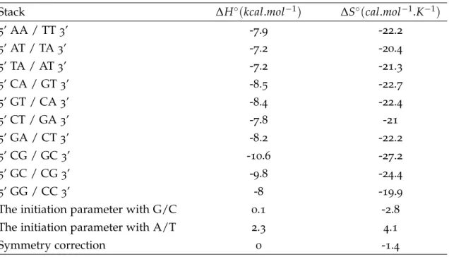
where R is the ideal gas law constant (1.987 cal/K·mol), [Na+] is the given sodium concentration,CTis the total oligonucleotide strand concentration (b=4, if the strands are in equal concentration). Thermodynamics parameters ∆H and ∆S each represents the enthalpy (the amount of heat energy possessed by substances) change and the entropy (the amount of disorder a system exhibits) change. The subscript ’d’ and ’i’ indicate the di-nucleotide pairs parameter values of each nearest neighbor base pair and the initiation parameter.∆S_{sel f} is the additional entropic penalty for the maintenance of the C2 symmetry of self-complementary duplexes. Values of the nearest-neighbor model parameters estimated in [22] are given in Table2.1.

Complexity and repetitive sequence

Given that DNA / RNA sequence are both composed of only 4 possible nucleotide bases, respectively, the chance of seeing some particular pattern of nucleotides, a k-mer,

(28)

Table2.1.:Nearest-Neighbor parameters for DNA/DNA duplex

Stack ∆H◦(kcal.mol−1) ∆S◦(cal.mol−1.K−1)

5’ AA / TT3’ -7.9 -22.2 5’ AT / TA3’ -7.2 -20.4 5’ TA / AT3’ -7.2 -21.3 5’ CA / GT3’ -8.5 -22.7 5’ GT / CA3’ -8.4 -22.4 5’ CT / GA3’ -7.8 -21 5’ GA / CT3’ -8.2 -22.2 5’ CG / GC3’ -10.6 -27.2 5’ GC / CG3’ -9.8 -24.4 5’ GG / CC3’ -8 -19.9

The initiation parameter with G/C 0.1 -2.8

The initiation parameter with A/T 2.3 4.1

Symmetry correction 0 -1.4

repeating itself somewhere else across all chromosomes is unsurprisingly high. Assum-ing that we are lookAssum-ing at a mammalian genome like human, which contains around 3×109nucleotide bases on a single strand, we want to know the probability of a 15bp (k=15) sequence P occurs only once in the whole genome. First, there are 4k different sequence formations, given only4possible bases to choose from. So for any specific lo-cation, the chance of seeing this particular15 bp sequencePis only 1/415=9.31E−10, which is not very likely. However there are N= 3E9 locations one could check against, which would lead to on average 3E9/415 = 2.79 occurrences of this pattern, and this is only counting one strand of the DNA. The chance of a single occurrence is there-fore(1−1/415)(3E9−1)_×₍_1/415₎_×₃_E₉ ₌ _{0.17. In probability theory and statistics, the} number of occurrence (X) of such a random pattern could be considered to follow a Binomial distribution, B(N,p), with the probability of exact matching p = 1/4k _and

the number of comparisons equals to N. Thus by applying the cumulative distribution function (CDF) of Binomial distribution, one can easily get the probability of having this sequence more than once in the genome, P(X >1) =1−P(X ≤1) =0.77, which is quite high. However when, k, the length of P increases, the success rate (p) drops exponentially, thus in turn the chance of having more than1occurrences decreases.

In real genomics, repetitive genomic sequences are sequences that show high degree of similarity or are identical to other parts of the genome. Their existences could be co-incidental combinatorial events or products of complex cellular mechanisms. However such repetitive sequences are observed more frequently than expected. Studies have

(29)

2.1. Custom tiling array design shown for well-characterized genome like human that, nearly 50% of human genome are covered by repeats [24; 25]. Such high degrees of repetitiveness are also present in other lines of organism; for example, in plants, arabidopsis [26] and maize [27] have been found to exhibit large scale genome wide duplication. In prokaryotic microorganisms, repetitive sequences are also detected at a large proportion [28].

For these repetitive sequences, further categorization could be made depending on their sizes, positions and structural adjacency. In general, there are two types of re-peats. Tandem repeats are those with the repeated copies in their immediate adjacency. Centromere and telomere of chromosome are largely comprised of tandem repeats. If the reoccurring copies of the transposable segments are located far from each other, they are termed as interspersed repeats. Due to the nature of complimentary base pairing of nucleotides, there is also another type of repeats, inverted repeats, which are sequences followed by their reverse complements, either immediately (tandem) or intervened by other random sequences (interspersed). When there is no intervening se-quence between the copies, this inverted repeat is also called palindromic. According to RepeatMasker [29; 30], classification of interspersed repeats can be further charac-terize by 4 sub-types, short interspersed nuclear elements (SINEs), long interspersed nuclear elements (LINEs), retrovirus-like elements or long terminal repeat (LTR) and DNA transposons. There are also many forms of tandem repeats, mainly characterized by repeat length, like microsatellites, minisatellites and satellites, which are frequently used as molecular markers in forensic science and population genetics studies.

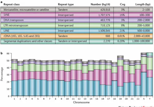
Most repeats are considered not functional, while some are involved in the evolution process [31;32;33], uncoupling intra- and inter-chromosomal gene conversion. Tandem repeats have also been shown to be associated with regulation of transcription factor binding [34], aging process [35], various disease forms including cancer [36; 37]. In-verted repeat and palindromic sequence, unlike most other types of repeats, are not well characterized by tools like RepeatMasker. Due to the special self-complementary structure, they can form secondary structure like stem-loop or hairpin, thus directly af-fecting genome stability [38]. In Figure 2.1, a summary of annotated human repetitive DNA reported by RepeatMasker are cited from [14].

Repetitive regions, as one major source of cross-hybridization and hybridization in-stablity, have been shown to account for a large proportion of mammalian genomes. For normal gene expression array and tilling chip used for transcriptom profiling, such repetitive segments are generally ignored in the probe selection process [13]. The most commonly adopted approach to handle repetitive regions is to exclude them using tools like RepeatMasker [29]or Window Masker [39]. However for tiling array, features re-side in the repetitive proportions identified by repeat masking tools may have particular

(30)

Figure2.1.:Summary of repetitive DNA sequences in the human genome (hg19)

significance [40]. Thus their inclusion should be considered in the chip design, and ef-forts have been made for the selection and interpretation of probes containing repetitive sequences [41;42].

Specificity and probe uniqueness

Probe specificity is the most crucial and problematic factor in microarray design, many experimental techniques and analytical methods have been developed to overcome this issue. Commonly, approaches to evaluate probe uniqueness are mostly alignment based, like using Basic Local Alignment Search Tool (BLAST) [43], other researchers also em-ploy suffix array [44] for faster indexing and matching. There are also attempts to ap-proximate the cross-hybridization potential using thermodynamic models to assess the binding-free energy between probes and non-targeted sequences [45]. Most of these de-velopments are done for the probe selection of gene expression array, where all known transcripts of the organism are targeted.

However when tackling tilling array designs, for mammals like us human (Homo sapi-ens), or other domestic animals like cow (Bos taurus) and pig (Sus scrofa), the total amount of DNA contained within one copy of a single genome is around3billion base pairs. To check if one particular query sequence is unique among the whole genome essentially involves approximately 2×3×109 comparisons, not to mention that for a high-density chip the number of probe sequence easily exceeds1million. For those alignment based

(31)

2.1. Custom tiling array design methods, repetitive searches are accumulatively slow and are not readily capable to han-dle large scale tiling tasks. A simplest form of suffix arrays for the reference genome can be implemented in1₈×n×log₂nbytes in space, which leads to a memory consumption of around23GB. Although those suffix array or suffix tree based approaches can deliver matched pattern in log-linear or linear time, the intensive memory usage could render most modern desktop PC infeasible. Thus a compressed index structure like Full-text index in Minute space (FM-index) [46], which is efficient in both query time and space consumption, is an ideal alternative for biological sequence analysis.

2.1.2. BWT and FM-index

FM-index is a compressed full-text sub-string index structure pairing the Burrows— Wheeler transform (BWT) [47] with suffix array, originally introduced by Ferragina, P. and Manzini, G.. The BWT was proposed by Burrows, M. and Wheeler, David J., which is a technique that reversibly rearrange the sequence in a way that similar characters from reoccurring subsequence would be sorted together. The nature of having consecu-tive runs of repeticonsecu-tive characters allows easy compression using schemes like run-length encoding (RLE).

Here I will first illustrate how BWT works and its pairing with suffix array via R code (see Appendix (A)). The R code here is only used for illustration purpose, thus may not be well optimized for real implementation. The transform function bwt() starts with appending an extra character like ’$’ , which is lexicographically smaller than any of the characters present in S, to the beginning of the input sequence S. Then construct a matrix M with rows representing all possible cyclic shifts of S, then have rows of M sorted lexicographically. The BWT transformation of the input, T, is then the last column of the sorted matrixM. The original sequenceS can also be reconstructed from the BWT transformed stringT, via the inversion functionibwt().

On the other hand, a suffix of S could be denoted as S[i,N], where i = 1, 2, . . . ,N, with the starting positionias pointer to each suffixS[i,N]. A suffix array could then be constructed by sorting all suffixes in the lexicographical order, and assign the associated pointer to each array element. The core of FM-index is the pairing of BWT with suffix array, their connection could be easily seen if we place the suffix array next to the BWT transformed sequence. The jth character in the BWT transformed sequence is just the character one position before thejth suffix. For example, consideringS =’mississippi’, the only ’m’ in the BWT encoded sequence T is ranked at the 5th position, while the corresponding suffix has an index of 2. The character before that suffix with index 2 is just the first character of the(2−1)th suffix which lies in the 6th row.

(32)

When looking at exact pattern matching problem, any matched pattern is essentially a prefix or a suffix of the full sequence. For a suffix array, since rows of suffixes have been sorted lexicographically, all occurrences of the pattern will be stacked together in consecutive rows. With the help of another two auxiliary data utilities,C andOcc, any suffix starts with the given query pattern can then be returned using backward search. C[c] is a look-up table containing the number of occurrences of characters in the full sequence which are alphabetically smaller than c. Occ(k,c)is a function which counts the occurrences of the charactercin thek-th prefix ofT,T[1,k]. Here I pre-computed all possible values ofOcc(k,c)as a matrix for the example sequence.

> occMat(bwt(exStr)) $ i m p s 1 | 0 1 0 0 0 2 | 0 1 0 1 0 3 | 0 1 0 1 1 4 | 0 1 0 1 2 5 | 0 1 1 1 2 6 | 1 1 1 1 2 7 | 1 1 1 2 2 8 | 1 2 1 2 2 9 | 1 2 1 2 3 10| 1 2 1 2 4

(33)

2.1. Custom tiling array design 11| 1 3 1 2 4 12| 1 4 1 2 4 > cMat(exStr) $ i m p s 0 1 5 6 8

For a query pattern P of length p, the start index s and end index e of the sorted suffix array which containsPcan be returned in a maximum of psteps. The searching starts with the last character of the query pattern, P[p], withs =1 and e = p. The two index are then iteratively recalculated using the following mapping scheme for each characterP[i]in the pattern,s′ = C[c] +Occ(s−1,P[i]) +1 ande′ = C[c] +Occ(e,P[i]). The mapping process is illustrated in the example below withP=’iss’. At the last step (p=3), the start and end index of suffix which starts with ’iss’ have been located,s=4 ande =5. S i T 0 1 2 3 1 | $ 12 i | s 2 | i$ 11 p | 3 | ippi$ 8 s | 4 | issippi$ 5 s | s 5 | ississippi$ 2 m | e 6 | mississippi$ 1 $ | 7 | pi$ 10 p | 8 | ppi$ 9 i | 9 | sippi$ 7 s | s 10| sissippi$ 4 s | 11| ssippi$ 6 i | s 12| ssissippi$ 3 i | e e e

2.1.3. Penalized uniqueness score

Gräf et al. [42] proposed the idea of using uniqueness score (U), which is the total number of minimum unique substring (MUS) in a given range, for cross-hybridization control in tiling probe selection. Following their original definition, a genome sequence in question is called G, which is a part of the whole genome assembly GS. If a substring X of G occurs only once in GS and each substring of X occurs more than once in GS, then this substring X is called a minimum unique substring (MUS) of G. At each position of G, if the substring from this position to the end of G is unique within GS, then there

(34)

exists one shortest unique prefix starting from that position, which is called a minimum unique prefix (MUP) at that position. The uniqueness score is then determined by counting the distinct end positions of MUP within the region.

> MUP(exStr, exStr) MUP.length m i s s i s s i p p i 1 *| 1 m 2 | 5 i s s i s 3 | 4 s s i s 4 *| 3 s i s 5 | 5 i s s i p 6 | 4 s s i p 7 | 3 s i p 8 *| 2 i p 9 *| 2 p p 10*| 2 p i 11 | 0

-In the code chunk above, using the same example string S from last section, the function MUPreturns the length of the MUP at each position for string ’mississippi’, with no MUP found at the last position. The searching of MUP takes the advantage of the relationship between suffix and prefix, since each prefix of the sequence is a suffix of the reversed sequence, and thus could be efficiently calculated with FM-index. Each minimum unique substring within are indicated by asterisk (∗). In real implementation, MUP are efficiently located via an external libraryGenomeTools[48].

However, in this definition of the uniqueness score, the author only considered the absolute number of MUS without accounting for the distribution of length and coverage within the probe range. Hypothetically, the first half of a probe could contain no MUS, while the remainder might harbor a large number of MUS (which could be up to the user-specified cut-off). In certain extreme cases, for longer oligonucleotide probes, the original definition would give a score higher than the specified threshold, even though the actual coverage of these MUS is only50%, and cross-hybridization could still occur. Another possible scenario is that compared to sequences with shorter MUS, probes with longer and near-window-sized MUS are more vulnerable to cross hybridization. A schematic illustration of the2aforementioned cases is shown in Figure2.2.

(35)

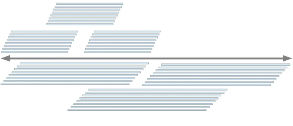
2.1. Custom tiling array design

Figure 2.2.: Schematic diagram of low MUS coverage and long MUS. Hypothetically

extreme cases showing low MUS coverage (above) and long MUS (below).

Hence the penalized uniqueness scoreUpis defined as the following in Equation (2.6),

Up=U×Cmus×(1−mean(Lmus)/Lmax) (2.6)

Cmus is the proportion of the probe covered by all MUS within. Lmus is the length of

individual MUS within the candidate probe. Lmax is the maximum possible length of

MUP, which defaults to30 and could be changed in the MUP searching step according to specific technical limits posed by the chip manufacture. U is the number of MUS within the candidate probe. So in the best case scenario, all MUS cover the whole probe and the coverage will induce no penalty on the uniqueness score. And regarding the average length of MUS, it will normally give a coefficient between 0 (only if all MUS within the probe have maximal length) and 1 (only when there is no MUS available). Thus as a rational number instead of integer count, theUp provides a wider dynamic

range.

To further illustrate the potential role of MUS coverage and length in probe unique-ness, the Agilent catalog array Human Whole Genome ChIP-on-Chip Set244K (available via Agilent’s eArray, see Appendix (B)) were fetched, which in total contains 5930500 probes spanning the whole human genome (hg19:GRCh37). All probes were processed for the two uniqueness scores and other oligonucleotide quality related measures. In ad-dition, BLAST-Like Alignment Tool (BLAT) [49] was used to find hybridization-quality alignments, which is defined as having at most one gap, at least 60% identity of the probe length, and gap length or mismatched bases not more than3. Such alignments are considered to be hybridized well, thus the number of qualified alignment could be

(36)

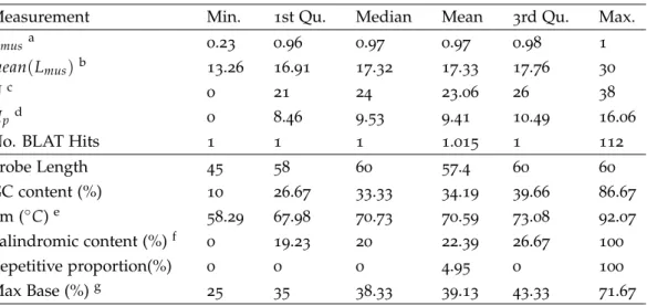
Table2.2.:Summary of Agilent ChIP-on-Chip Set probe properties Measurement Min. 1st Qu. Median Mean 3rd Qu. Max.

Cmusa 0.23 0.96 0.97 0.97 0.98 1

mean(Lmus)b 13.26 16.91 17.32 17.33 17.76 30

Uc 0 21 24 23.06 26 38

Upd 0 8.46 9.53 9.41 10.49 16.06

No. BLAT Hits 1 1 1 1.015 1 112

Probe Length 45 58 60 57.4 60 60 GC content (%) 10 26.67 33.33 34.19 39.66 86.67 Tm (◦C)e 58.29 67.98 70.73 70.59 73.08 92.07 Palindromic content (%)f 0 19.23 20 22.39 26.67 100 Repetitive proportion(%) 0 0 0 4.95 0 100 Max Base (%)g 25 35 38.33 39.13 43.33 71.67

a_{the percentage of the probe region covered by MUS} b_{the average length of all MUS within the probe} c_{the original uniqueness score}

d_{the penalized uniqueness score}

e_{the melting temperature evaluated using Equation (}2.5)

f _{maximal proportion of inverted repeat (IR)} g_{maximal proportion of the four nucleotide bases}

used as an indicator for cross hybridization potential. According to the chromosomal co-ordinates provided in the GEO files shipped together, probes were back-mapped to the same version of RepeatMasker-masked genome sequence (hg19:GRCh37). Proportion of masked bases was calculated for each mapped probe.

In Table 2.2, the calculated probe characteristics are summarized, which gives an overview of the general probe quality of the chip (figures of all parameters’ distribution could be found in Additional files of [9]. In general, the catalog probes show similar hy-bridization efficiency, with an inter quartile range of melting temperature from 67.98◦C to 73.08◦C; low cross hybridization potential, with an average uniqueness score (U) of 23.06 (median24) and the penalized uniqueness score (U_p) of9.412(median 9.53); lim-ited self-hybridization potential, having a mean palindromic content of22.39% (median 20%). Back-mapping of Agilent chip targets to the reference sequence also suggests in-clusion of repetitive sequence, with411292probes having repetitive proportion greater than zero, and199471probes being completely masked as repetitive.

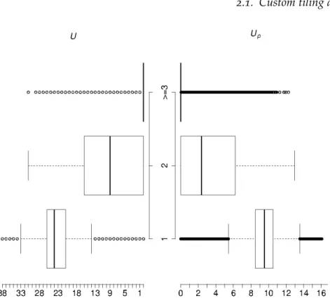
After BLAT alignment, 99.4% of the probes found to have unique quality alignment, while only34274 probes had been mapped to multiple locations. A back-to-back box-plot (Figure2.3) was made for the two scores to visualize the general group differences

(37)

Figure2.3.: Back-to-back box-plot of original uniqueness score (U, left) and the penal-ized uniqueness score (Up, right) distribution within different BLAT hits groups (1, aligned to1position;2, aligned to2positions;≥3, aligned to at least3positions)

in their distributions. Both plots show similar overall pattern, probes with unique align-ment tend to have higher scores than those with multiple hits. A visible difference of the grouping effect between the two scores could be found that, for the penalized uniqueness score the difference of median between group2 and3 is much lower than the difference of median between group2and group1.

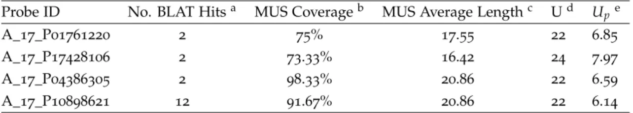
In Table2.3, some exploratory probes are selected from this chip which are potentially vulnerable for cross-hybridization. The four 60 bp probes all show relatively high U values, close to the average level (mean=23.06, median=24) of all probes on the chip, and multiple quality alignments. The first two probes show relatively low coverage, which are far below the first quantile of all probes. The other two probes show relatively long average MUS length, which are above the third quantile (17.76) of all probes. However, when looking at the penalized uniqueness score, all four of them exhibit relatively low level ofUp, below the first quantile (8.46) of all probes on the chip. It is then suggestive that the penalized uniqueness score is more sensitive in assessing cross-hybridization potential, when taking into account of the size and positional distribution of MUS in the analysis.

(38)

Table2.3.:Example of problematic60-mer probes from Agilent ChIP-on-Chip Set Probe ID No. BLAT Hitsa MUS Coverageb MUS Average Lengthc Ud Upe

A_17_P01761220 2 75% 17.55 22 6.85

A_17_P17428106 2 73.33% 16.42 24 7.97

A_17_P04386305 2 98.33% 20.86 22 6.59

A_17_P10898621 12 91.67% 20.86 22 6.14

a_{Number of hybridization-quality alignment to the reference genome.} b_{The percentage of the probe region covered by MUS.}

c_{The average length of all MUS within the probe.} d_{The original uniqueness score.}

e_{The penalized uniqueness score.}

2.1.4. Tiling probe selection algorithm

Tiling probes can be selected in the most straightforward way, either using an end-to-end fashion or with a fixed distance or overlap between neighboring tiles. However, these simple strategies will easily encounter problems like cross-hybridization and low hybridization potential, problems that would eventually contaminate the data. Also, instead of having a high coverage up to100% initially, the number of probes with valid signals could fall significantly after data processing. Thus an optimized and uniform tiling path is highly desirable [13]. Most of the available methods employ a window approach, which first divide the whole target region into non-overlapping fixed-size windows, and then select optimal probes within each window. Thus the resolution of the probe mapping will depend on the initial window size, this approach is preferred in CHIP-on-chip design when studying protein-DNA interaction or when high probe density is not of interest. However when mapping transcriptome, overlapping probes will provide better resolution in locating exon boundaries. To gain more control of the expected quality while giving better resolution and coverage, the following design strategy and pipeline which embed the previously defined penalized uniqueness score is presented. Full selection parameters could be seen in Table2.4.

The algorithm, namelyOTAD, searches for candidate probes in an intuitive growing fashion, from the 5’ of the sequence to the 3’ end. In general, neighboring probes is made to have a fixed size of overlap, if the targeted probe satisfied the user-specified constraints. Otherwise, the adjacent positions overlapping with 1 nucleotide more or less would be tested, and the search would keep shifting until the next valid probe is found or the boundary of the genomic region is reached. The shifting and checking is done intelligently to avoid unnecessary calculation.

(39)

Table2.4.:Parameters of tiling probe selection algorithm Parameter Type Description

-h print help

-P Integer maximal parallel process (default: 1)

-f Directory path of folder containing fasta files with extension ’.(m)fa(.gz)’ -w Char strand to be designed ’b’ (both), ’+’, or ’-’ (default: +)

-l Integer maximal length of the probe (like:60)

-v Integer maximal shrinking of probe length (default: 0)

-o Integer maximal length of overlapping (like: 20)

-u Integer minimal uniqueness score (like:21)

-U Real minimal penalized uniqueness score (like: 9)

-T Real range of Tm calculated with nearest-neighbor model (like: 70-80)

-G Real range of GC content (default: 0.2-0.6)

-s Integer maximal single nucleotide repeats (default: 6)

-d Integer maximal di-nucleotide repeats (default: 4)

-b Real maximal proportion of each bases (default: 0.6)

-c Integer maximal number of synthesis cycles allowed (default: 148)

-p Real maximal proportion of palindromic sequence (like: 0.3)

-r Real maximal proportion of repetitive masked bases (like:0.1)

then the files in the input folder must contain ’mfa(.gz)’

Pseudo code of the detailed selection mechanism is shown in Appendix (C). An evenly-spaced, non-overlapping tiling path can also be achieved by specifying a neg-ative value for the overlap size. Another separate option of variable probe length can be combined with the overlapping option to compensate for coverage in regions where fixed-length probes cannot be placed. The variable length design is also advantageous in selecting isothermal probes to reduce sequence bias [15]. Strand-specific design is also possible; if both strands are present on the same array, offsets between reverse complimentary tiles on the two strands are determined internally.

2.1.5. Penalized uniqueness score evaluation

Comparison of sensitivity and specificity

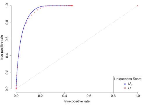
To further validate and evaluate the relative performance of the penalized uniqueness score against the uniqueness score, the previously processed Agilent Human ChIP-on-Chip Set was used. Receiver operating characteristic (ROC) measuring the trade-off between sensitivity and specificity was adopted to directly compare the discrimina-tive power in non-unique probe classification. After the BLAT alignment, number of

(40)

hybridization-quality alignment was determined for each probe. In order to construct the curve, a series of values ranging from the minimum to the maximum of the unique-ness score are used as cut-offs to predict whether the probe has only one hybridization-quality alignment or more. If the probe has a uniqueness score higher than the cut-off, then it is classified as positive and estimated to have only one quality alignment, and negative otherwise. Sensitivity is defined as the true positive rate (TPR), which is the number of probes identified as positive and indeed having only one quality alignment divided by the number of probes with an alignment score equalled to one. Specificity is defined as1minus the false positive rate (FPR), which is the number of probes iden-tified as positive but having more than one quality alignment divided by the number of probes actually having one quality alignment. Curves for both scores are overlaid in Figure2.4. It could be seen that both scores work quite well and strongly deviate from the diagonal. However a visible trace of difference could be observed at the upper left corner, suggesting a clear gain of advantage by the penalized uniqueness score.

Figure 2.4.: ROC curves of using original uniqueness score (U, red) and the penalized

uniqueness score (Up, blue) for BLAT hits group classification.

Benchmarking of public array data

To further illustrate the discriminative power of the penalized uniqueness score, ar-ray data from public repository were evaluated. One popular platform from Agilent

(41)

2.1. Custom tiling array design was chosen, human whole-genome expression array4x44K (ArrayExpress platform ID: A-AGIL-28), which contains41000unique probes. 14single color array datasets are ran-domly selected from this platform, all having proper replicate (at least2) for each factor level. Probes were scored using the penalized uniqueness score. For each experiment, like running a practical microarray analysis, pre-processing and filtering were done us-ing Bioconductor[50] packageAgi4x44PreProcessPedro Lopez-Romero [51]. Experimen-tal designs were derived according to individual experiment description. Procedural and parametric settings of background-correction, normalization and filtering were set to default, and common to all experiments. The filtering in Agi4x44PreProcessis done sequentially: first, control probes are filtered; then probes with signal not well above the local background are filtered; the third criteria is by the Agilent’s FeatureExtraction flag ’gIsFound’; for the next step, probes with signal not well above the negative controls are filtered. So far, the remaining probes all have detectable and valid signal. In the next stage, over-saturated probes are removed, which could be linked to severe cross-hybridization or possible contamination to the slide; In the end, population outliers and non-uniform outliers are filtered, which could also be related to cross-hybridization or other variations in experimental conditions. In this work, probes filtered out in the last2 stages were considered as potential victims of cross-hybridization and had them further investigated for uniqueness.

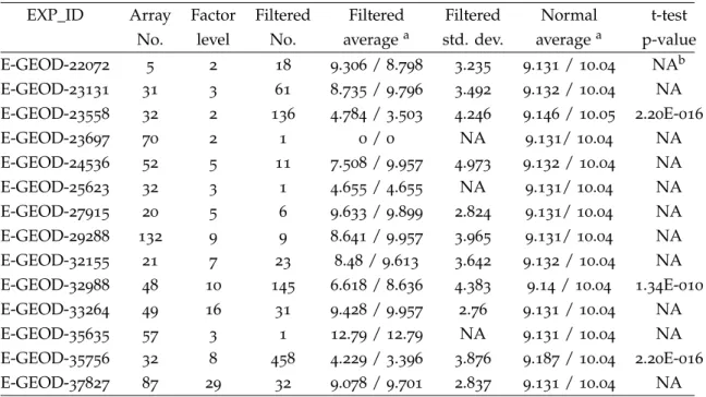
Table2.5.:Summary of experiments from ArrayExpress

EXP_ID Array Factor Filtered Filtered Filtered Normal t-test No. level No. averagea std. dev. averagea p-value E-GEOD-22072 5 2 18 9.306/8.798 3.235 9.131/10.04 NAb E-GEOD-23131 31 3 61 8.735/9.796 3.492 9.132/10.04 NA E-GEOD-23558 32 2 136 4.784/3.503 4.246 9.146/10.05 2.20E-016 E-GEOD-23697 70 2 1 0/0 NA 9.131/10.04 NA E-GEOD-24536 52 5 11 7.508/9.957 4.973 9.132/10.04 NA E-GEOD-25623 32 3 1 4.655/4.655 NA 9.131/10.04 NA E-GEOD-27915 20 5 6 9.633/9.899 2.824 9.131/10.04 NA E-GEOD-29288 132 9 9 8.641/9.957 3.965 9.131/10.04 NA E-GEOD-32155 21 7 23 8.48/9.613 3.642 9.132/10.04 NA E-GEOD-32988 48 10 145 6.618/8.636 4.383 9.14/10.04 1.34E-010 E-GEOD-33264 49 16 31 9.428/9.957 2.76 9.131/10.04 NA E-GEOD-35635 57 3 1 12.79/12.79 NA 9.131/10.04 NA E-GEOD-35756 32 8 458 4.229/3.396 3.876 9.187/10.04 2.20E-016 E-GEOD-37827 87 29 32 9.078/9.701 2.837 9.131/10.04 NA

a_Up_{average column is formated as ’mean / median’.}

(42)

In the end, summary statistics of the penalized uniqueness score for filtered probes were derived, in Table2.5, which are over-saturated or outlying and thus could be re-lated to cross-hybridization. For the analyzed experiments, the number of probe filtered varies from1to458. Interestingly, for all except one experiment (E-GEOD-35635), those filtered-out probes exhibit lower average Up score and thus are less unique according

to the uniqueness measurement. Difference in group mean of penalized uniqueness score was assessed using formal statistical test. In order to achieve statistical power of 0.9 when using a two sided t-test to detect a mean difference of 0.5with standard de-viation of 1, it would require at least 85 observations in each sample. Therefore t-test are only performed for those experiments which has more than 85 probes filtered out. For all three qualified experiments, significantly lower uniqueness are detected for those filtered-out probes. So re-analyzing public array data provided further support of us-ing the penalized uniqueness score to discriminate non-specific probes for microarray design and data analysis.

2.1.6. Design comparison with commercial array

To address the coverage and resolution of the proposed probe selection pipeline, once again the previously processed Agilent Human ChIP-on-Chip Set was used. To simplify the comparison, only those probes targeting chromosome22(GenBank: NC_000022.10) were chosen rather than the whole set. The reference genome sequence was downloaded from the NCBI archive. Knowing that, for experiments like CHIP-chip, the sheared chro-matin fragment is generally around500bp [52], using short oligonucleotides (<100-mer) makes it more cost-efficient to choose an optimal distance between tiles than to solely increase the number of probes and the tiling density. To compare with Agilent’s catalog design, the distribution of the distance between neighboring tiles in the catalog array is summarized, with a median of 202 nucleotides and a mean of 426 nucleotides be-tween adjacent probes. The probe length also varies, ranging from 45-mer to 60-mer (median=53 and mean=52.85). With the proposed implementation, several overlapping sizes (from -325nt to -250nt) have been tested to make the overall probe number close to the Agilent catalog design. The minimum probe length was set to 45-mer, while initial probe length always starts at 60- mer. For probe melting temperature, in Gräf et al. [42] they used the simple GC model like Equation (2.4) and tested two ranges of temperatures, 73−76◦Cand 77−80◦C, which in turn correspond to a GC content range of around30-50% for a50-mer oligo. In contrast, by considering the Tm distribution in the Agilent catalog array, a Tm range of 69−74◦Cwas selected for the nearest neighbor model Equation (2.5) and combined with a controlled GC content range of 30-50% as the criteria for optimal hybridization efficiency. For cross-hybridization control, a

(43)

pe-2.1. Custom tiling array design nalized uniqueness score of9was used as the empirical cut-off. A threshold of30% for palindromic content was used, while all other parameters were kept as the following: no base proportion higher than60%, single nucleotide repeats not exceeding6 and not having more than4di-nucleotide repeats.

With the proposed implementation, it took around2hours on a3.0Ghz single core PC to finish the process, without enabling the parallel mode. In Table2.6, the Agilent cata-log design and several custom designs are summarized, showing that the proposed flex-ible strategy could achieve higher coverage with fewer and, on average, longer probes. The coverage was assessed using two types of measurement, the raw non-redundant bases covered (ambiguous base ’N’ adjusted) and the total length of unit-sized (1000bp) windows in which at least one probe was placed.

Table2.6.:Design summary and coverage comparison

Design Probe No. Probe Len.c _{Inter-Probe Dist.}d _{Base Coverage} _{Window Coverage}e

Agilenta 73373 53/52.85 202/426 11.11% 51.25%

-o -250b 75036 60/57.16 246/411.9 12.29% 53.60%

-o -275 72087 60/57.11 269/431.1 11.80% 53.66%

-o -300 69491 60/57.02 292/449.4 11.35% 53.74%

-o -325 67074 60/56.92 313/467.7 10.94% 53.81%

a_{Agilent Human Whole Genome ChIP-on-Chip Set}244K (Chromosome22only)

b_{Overlapping size set to -}₂₅₀_{, probe length range [}₄₅_,₆₀_{], Tm range [}₆₉_,₇₄_],_Up_{range [}₉_{, Inf),}

palindromic content range [0,30%], GC content range [30%,50%]

c _{Average probes length in nucleotide, cell is formatted as median / mean} d_{Average inter-probe distance in nucleotide, cell is formatted as median / mean}

e _{Using the length of all unit-sized (}1000bp) windows in which at least one probe was placed

2.1.7. Uniqueness of palindromic sequence

With increasing potential for self-hybridization, palindrome sequences play an impor-tant structural role in the biogenesis of microRNA [53;54;55] and also have other func-tional characteristics like acting as restriction enzyme sites [56]. Interestingly, unlike in Gräf et al. [42], where the author claimed that palindromic sequences are more unique in the genome, an opposing relationship between palindromes (measured as the maximal proportion of inverted repeat) and uniqueness are observed (Figure2.5): Agilent’s cata-log probes with higher palindromic content tends to have lower mean uniqueness scores, which causes a left-shifting of their distributions when using a high palindrome cutoff. Small yet significant correlations could also be detected for both uniqueness scores [U, -0.0736428 (p<2.2e-16); U_p, -0.1050423 (p<2.2e-16)] and BLAT hits [0.00209 (p=3.578

(44)

e-07)] with palindromic content. However, the distribution of BLAT scores is extremely left-tilted, since most probes are aligned only once, therefore, despite supporting our findings, the correlation test may not be valid.

Figure2.5.:Distributions of the original uniqueness score (U, left) and penalized unique-ness score (Up, right) of the Agilent Human Whole Genome ChIP-on-Chip Set244K (1to25) probes, using different level of palindromic content as cut-off.

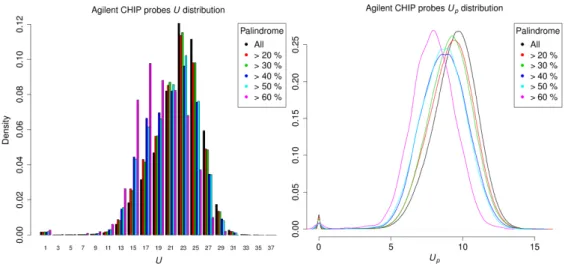
To investigate further the relationship between sequence uniqueness and palindromic content, data from a separate experiment were utilized, in which the proposed imple-mentation has been used to design tiling arrays for several chromosome regions of the pig genome. For one of them, on Sus Scrofa chromosome14 (GenBank: NC_010456.3) from 74377028 bp to 78176022 bp, the profiles of previously listed design parameters were evaluated for all possible 60-mer probes in the indicated region. In total 3328358 candidates were evaluated.

For the two uniqueness scores (Figure 5), unlike for the Agilent catalog array, their distributions are far from normal, both having a peak at zero and a flat, uniform interval followed by a narrow, bell-shaped region. This "twin-peak" distribution makes any formal statistical tests infeasible. However, by thresholding on palindromic content, the density of uniqueness scores were determined for candidates with palindromic content higher than the cut-off; in this way, sequences with higher palindromic content are directly visualized, which are subject to removal in the probe selection process. When using a higher cut-off of palindromic content, the trend of differences resembles that observed for the Agilent chip: the density curves tilt left, with both peaks shrinking and the saddle region raising. In particular, the proportion of sequences with close to 0 uniqueness score remains large in the high-palindrome group (>60%), yet the high

(45)

2.1. Custom tiling array design uniqueness peak vanishes.

Figure 2.6.: Distributions of the original uniqueness score (upper-left) and penalized

uniqueness score (upper-right) using different level of palindromic content as cut-off for60-mer candidate probes on pig chromosome14(Sus ScrofaBuild10, NC_010456.3) region from 74377028 bp to 78176022 bp, and on the lower panel shows their distri-butions after filtering with standard probe selection criteria.

Finally, candidates violating those probe selection parameters were further filtered out, which include a narrow band of melting temperature (69−74◦C), moderate GC content (30%-50%), no base exceeding 60%, and no single and di-nucleotide repeats exceeding the thresholds of 6 and4 respectively. After filtering, a similar pattern per-sists, yet is not so pronounced, suggesting that the filtering removed more candidates with low uniqueness scores. One particular feature is that the candidates with high palindrome (>60%) and0uniqueness scores were removed by filtering.

(46)

The results suggest that with higher palindromic content the sequence tends to have a lower uniqueness score, contrary to what has been previously claimed in [42]. Aside from nucleotide sequence, studied the palindrome in protein sequence using a linguistic measurement, in which they also related palindromes with low sequence complexity. Under the defined uniqueness measurement, lower complexity normally leads to fewer and longer MUS in the region, resulting in a lower penalized uniqueness score. The experimental observations made here could also be explained in plain theory, since a highly palindromic sequence will share a large identical segment with its reverse complement strand; thus there should be fewer unique substrings found in such regions.