C
ALCULATION OF
V
ALUE
-
AT
-R
ISK AND
E
XPECTED
S
HORTFALL
UNDER MODEL UNCERTAINTY
A
LEXANDRA
B ¨
OTTERN
Master’s thesis
2015:E37
Faculty of Engineering
Centre for Mathematical Sciences
Mathematical Statistics
C
E
N
T
R
U
M
S
C
IE
N
T
IA
R
U
M
M
A
T
H
E
M
A
T
IC
A
R
U
M
Abstract
This thesis studies the concept of calculation of Value-at-Risk and Ex-pected Shortfall when the choice of model is uncertain. The method used for solving the problem is chosen to be Bayesian Model Averaging, using this method will reduce the model risk by taking several models into ac-count. Monte Carlo methods are used to perform the model averaging and the calculation of the risk measurements.
A NIG-CIR process is used to generate the data that is to be consid-ered unknown, for which Value-at-Risk and Expected Shortfall is to be calculated. It is chosen since it have behaviour that often occur in finan-cial data. The model averaging is performed using six different processes of varying levels of complexity. Both a weighted average based on BIC and a equally weighted average is calculated for the two risk measurements. The more complex models that are used in the Bayesian Model Averag-ing is GARCH processes, an EGARCH process and a stochastic volatility model, namely the Taylor 82 model. The methods used for parameter estimation are Maximum likelihood estimation and Kalman filtering.
The results in this thesis clearly shows that it is advantageous to cal-culate Value-at-Risk and Expected Shortfall using model averaging. But there is not any clear conclusion on which weights that give the most accurate estimate. But considering the time and effort that goes in to calculating the weights, using equal weight seems preferable.
Preface
Deciding on a topic for my Master thesis was a tricky decision. But after talking to my supervisor assoc. prof. Erik Lindstr¨om, and he presented the idea for this thesis, I made my decision. I found this topic interesting for many reasons, one of them was that the concept of averaging over several models to get better a result felt intriguing.
To average over several values is something we are taught from an early age and to use this concept to better model unknown data was something I found interesting. Of course it was not as easy to calculate the model average as it was to calculate the averages one did when growing up, but that is what makes the process interesting. Another thing I found interesting is that although the area of application in this thesis was towards financial risk measurements, the concept of model averaging is possible to apply in many different areas of study. I have learnt a great deal during this thesis, both knowledge wise and about myself as a person. I would like to begin by thanking my supervisor Erik Lindstr¨om for introducing me to this project but also for your support and guidance during this project. Secondly I would like to thank my family and friends for their support during this time, your support have made this process a lot easier.
I do hope you find the contents of this thesis interesting and to get a brief overview of the topic I would recommend to read the abstract.
Contents
Abbrevations 1
1 Introduction 2
1.1 Problem formulation . . . 2
2 Theory 3 2.1 Stylized facts of financial data . . . 3
2.2 Value at Risk & Expected Shortfall . . . 4
2.3 Bayesian Model Averaging . . . 5
2.4 Bayes Information Criterion . . . 6
2.5 Mathematical methods . . . 8
2.5.1 Monte Carlo Methods . . . 8
2.5.2 Maximum likelihood estimation . . . 10
2.5.3 Kalman Filter . . . 10
2.6 Different mathematical models . . . 11
2.6.1 NIG-CIR . . . 11
2.6.2 GARCH & EGARCH . . . 13
2.6.3 Stochastic Volatility model - Taylor 82 . . . 18
3 Simulations 19 3.1 Creation of the NIG-CIR data . . . 19
3.2 Fitting distributions to the data . . . 22
3.3 BMA . . . 30
4 Results 33 5 Conclusions 40 Appendices 41 A Derivation of the Hessian matrix - MLE . . . 41
A.1 Normal distribution . . . 41
Abbrevations
ACF Auto Correlation Function.
ARCH Autoregressive Conditionally Heteroscedastic.
BIC Bayesian Information Criterion.
BMA Bayesian Model Averaging.
CIR Cox-Ingersoll-Ross.
EGARCH Exponential GARCH.
ES Expected Shortfall.
FSA Fishers Scoring Algorithm.
GARCH Generalized Autoregressive Conditionally Heteroscedastic.
MLE Maximum Likelihood Estimation.
NIG Normal Inverse Gaussian.
SV Stochastic Volatility.
SWN Strict White Noise.
1
Introduction
A problem one never eludes when having unknown data is the process of se-lecting an appropriate model to describe the data. This decision will affect the future results that the calculations based on the selected model yields. To choose an appropriate model is a task that has proven to be difficult and there are several different model selection processes that are regularly used. Despite this, it still is not always enough to get a good model for the data.
When faced with financial data, the data often demonstrates several complex behaviours such as skewness and volatility clustering [5]. Choosing one single model to represent this data will with a high probability prove to be inadequate to use for some purposes, this is a problem called model risk. There are several risk categories often defined in finance i.e. market risk, credit risk and opera-tional risk. The notation of model risk is one that occurs in almost all areas of risk.
This thesis will focus on the two risk measurements Value-at-Risk and Ex-pected Shortfall. Value-at-Risk is one of the most widely used risk measures and is mentioned in Basel II that is recommended to use for calculation of market risk. But due to that Value-at-Risk have problems capturing behaviours such as tail risk, it is in Basel III recommended that Expected Shortfall is to replace VaR. Expected Shortfall is closely related to Value-at-Risk and is becoming more popular as time passes as it is a coherent risk measure. Nevertheless there are some problems with the risk measurements, one of these is model risk. Model risk is the risk that a financial institution obtain losses, due to that their risk-models are misspecified or the underlying assumptions of the model might not be met. For example, if one tries to model losses using a Normal distribution, the occurrence of volatility clustering might go unrecognized by the model.
The most standard practise in statistics is to choose one model that suppos-edly is the one that has generated the data. However this approach disregard the fact that the chosen model might not be, or even most certainly, is not the true model. Consequently rendering an over-confident model which in turn might lead to greater losses due to taking riskier decisions. A way to reduce the model uncertainty, therefore reducing the model risk, is to use model averaging. Bayesian Model Averaging is the method considered in this thesis. By averag-ing over several different models the positive contribution from each model will contribute to the final result, thus yielding a less uncertain measure.
1.1
Problem formulation
Deciding on how to carry out this thesis began by deciding on some main points, i.e. which data should be used to perform the analysis and which method should be used to perform the modelling.
It was decided that a NIG-CIR process should be used as a data source during the simulations and that this data was to be considered unknown. The NIG-CIR process were chosen due to that it has several properties that are common to financial data.
The next problem was to decide on which models that were to be fitted to the data. It was decided to use two simpler models, the Normal distribution and the Student’s t distribution, but also three more complex processes. These three processes are a GARCH process, an EGARCH process and a Stochastic Volatilty model, Taylor 82 model. Fitting these distributions to the data is another topic in this thesis.
The final step is to use these processes to generate the Bayesian Model Av-eraging estimates of the Value-at-Risk and Expected Shortfall estimates. The calculation of the estimates will be performed using Monte Carlo methods. The idea is to show that by averaging over several different models instead of choosing one single model, the estimate will be more accurate. There will be a compari-son between an equally weighted average and a weighted average, where it was decided that the weights were to depend on Bayes Information Criterion, more details on the weights can be seen in 2.3.
2
Theory
2.1
Stylized facts of financial data
Financial data have some special properties that is unusual in other data types. These so called stylized facts are based on empirical observations of financial data [1]. There are several different ones, some of them are mentioned below
• Little to no autocorrelation in the return series
• Conditional expected returns close to zero
• The return series has heavy tails and/or is leptokurtic
• The return often shows signs of skewness
• Volatility clustering often exists
• The absolute value or square of the returns have a clear serial correlation. This is the so called Taylor effect.
Heavy tails & leptokurtosis
The Gaussian distribution is often a poor fit for financial data, the data con-tains much more extreme events than the Gaussian distribution can predict. In general, financial return data seems to have a higher kurtosis than the Gaussian distribution, it is hence said to be leptokurtic. A distribution that is leptokurtic has a higher peak in the middle and heavier and longer tails [1]. This behavior of the data make for a problem when calculating Value at Risk and Expected Shortfall using a Gaussian distribution. When calculating VaR and ES using a Gaussian distribution fitted to financial data, the estimates will be overesti-mated on low confidence levels and underestioveresti-mated on high confidence levels[15]. This is because the financial data have heavier tails than the Gaussian distri-bution have the ability to predict.
Volatility clustering
Volatility clustering is a phenomenon often occurring in financial data. This means that one extreme return often is followed by one or more extreme re-turns, not necessarily with the same sign [1]. That a process is heteroscedastic means that the volatility of the process changes over time. Most heteroscedastic processes contains volatility clusters, examples of these are ARCH and GARCH processes which will be presented in 2.6.2.
2.2
Value at Risk & Expected Shortfall
Value-at-Risk (VaR) [1] is a commonly used risk measure in financial insti-tutions. And as mentioned before, it is the risk measurment that Basel II recommend shall be used for calculating market risk.
Consider a fixed time horizon ∆ the loss distribution and the loss distributions distribution function is then defined according to
L[s,s+∆] :=−(V(s+ ∆)−V(s))
FL(l) =P(L≤l)
(1)
The VaR-measure is calculated as the quantile function of the loss distribu-tion, given a confidence level α, α ∈ [0,1]. In other words it is the smallest valuelsuch that the lossLis not greater thanlwith a probability (1−α). The expression of the VaRαis shown in equation (2)
VaRα= inf{l∈(R) :P(L > l)≤1−α}
= inf{l∈(R) :FL(l)≥α}=qα(FL)
(2)
whereqα(FL) denotes the quantile function. VaR is not a coherent risk
mea-surement, meaning it does not behave in the way we would have wanted. In order for a risk measure % to be coherent it needs to satisfy the four axioms of coherence. The axioms of coherence for a risk measure% :M → R on the convex coneM, follows below
1. Translation invariance.
For allL∈ Mand everyl∈Rwe have %(L+l) =%(L) +l
2. Subadditivity.
For allL1, L2∈ Mwe have %(L1+L2)≤%(L1) +%(L2)
3. Positive homogeneity.
For allL∈ Mand everyλ >0 we have%(λL) =λ%(L) 4. Monotonicity.
ForL1, L2∈ Msuch thatL1≤L2 almost surely we have %(L1)≤%(L2)
VaR does not satisfy all the axioms of coherence, it does not satisfy the axiom of subaddidivity, and thus is not a coherent risk measure. Expected shortfall on the other hand does satisfy all criteria to be coherent. In Basel III it is recommended that ES shall replace VaR for calculation of market risk since ES is able to capture some behaviours VaR can not, i.e. tail risk. Due to this to study both Expected Shortfall and Value-at-Risk in this thesis.
Using the definitions of the loss distribution as in (1) whereE(|L|)<∞the expected shortfall at confidence level α∈ (0,1) is defined as in (3) if the loss distribution is continuous
ESα=
E(L;L≥qα(L))
1−α =E(L|L≥VaRα) (3)
That is, the expected loss given that VaR is exceeded. Another definition that often is used is
ESα= 1 1−α Z 1 α qu(FL)du = 1 1−α Z 1 α VaRu(L)du (4)
It can be interpreted as that expected shortfall is calculated by averaging VaR over all levelsu≤α.
2.3
Bayesian Model Averaging
Bayesian model averaging is a mathematical method, originating from Bayes formula. It assumes that there is a set of different modelsM1, ..., Mk, that all are
a fairly good fit for estimating the quantityµfrom the datay[9]. The parameter
µis defined and has an interpretation that is common for all the models. Instead of using just one of these models, Bayesian Model Averaging (BMA) constructs
π(µ|y), which is the posterior density of µ given y, unconditioned on any of the models. BMA begins by specifying the prior probabilities,P(Mj), for the
different models and by specifying the prior densities,π(θj|Mj), whereθj is the
parameters of modelMj. The integrated likelihood of modelMj is then given
P(Mj|y)∝λn,j(y) =
Z
Ln,j(y, θj)π(θj|Mj)dθj (5)
WhereLn,jis the likelihood function for modelMjandλn,j(y) is the marginal
density of the unobserved data. Using Bayes theorem yields the posterior density of modelMj as (6) P(Mj|y) = P(Mj)λn,j(y) Pk j0=1P(Mj0)λn,j0(y) (6) The next step is to calculate the posterior density ofµ, this can be done as in (7) π(µ|y) = k X j=1 P(Mj|y)π(µ|Mj, y) (7)
This means that instead of assuming one model to be true, the posterior density in (7) is a weighted average of the conditional posterior densities. The weights are the posterior probabilities of each model. Since the method does not condition on any given model, it does not ignore the problem of model uncertainty. The posterior mean and posterior variance can be calculated as in (8) and (9) respectively [9]. E(µ|y) = k X j=1 P(Mj|y)E(µ|Mj, y) (8) V(µ|y) = k X j=1 P(Mj|y) V(µ|Mj, y) + (E(µ|Mj, y)−E(µ|y)) 2 (9) In this thesis the quantity µ is VaR and ES and the average is calculated using Monte Carlo methods. The weight forMj will be calculated as,
wj=e−BIC/2 (10)
which is the posterior model probability seen in (6) and the integrated likeli-hood in (5) is calculated as the approximate BIC seen in (21). Averaging over all considered models has been shown to provide a better predictive ability in average, measured using a logarithmic scoring rule, than using one single model
Mj conditional on all considered models [11].
2.4
Bayes Information Criterion
The Bayesian Information Criterion (BIC) is a measurement on how good es-timate fit a model is and it is a way of deciding which model is the best fit to the data. The BIC is a measurement which punishes model complexity using a Bayesian framework [9]. The criterion takes the form of a penalised log-likelihood function as seen in (11).
BIC(M) = 2logL(M)−log(n)dim(M) (11) WhereM is the model, dim(M) is the number of parameters that is estimated in the model andnis the sample size of the data set. The model with the largest BIC value is the one that is the best fit. The Bayesian approach to model selection, is to select the model that out of several models is the one which is a posteriori the best fit. The posterior probabilities of models,M1, ..., Mk, derived
from Bayes theorem is shown in (12)
P(Mj|y) = P(Mj) f(y) Z Θj f(y|Mj, θj)π(θj|Mj)dθj (12)
where Θj is the parameter space andθj∈Θj andy1, ..., yn is the data. P(Mj)
is the prior probability of model Mj, f(y) is the unconditional likelihood of
the datay, f(y|Mj, θj) = Ln,j(θj) is the likelihood function for the data and
π(θj|Mj) is the prior density ofθjgiven the data. The unconditional likelihood,
f(y), is computed from (13) f(y) = k X j=1 P(Mj)λn,j(y) (13)
λn,j is the marginal likelihood of modelj withθj integrated out with respect
to the prior, as seen in (14) [9]
λn,j=
Z
Θj
Ln,j(θj)π(θj|Mj)dθj (14)
When comparing the posterior probabilitiesP(Mj|y) with respect to the
dif-ferent models, the unconditional density f(y) is irrelevant since it is constant across the models, it isλn,jthat is important to evaluate. Define the exact BIC
estimates, BICexactn,j , as (15), yielding the posterior probabilities in (16) [9]
BICexactn,j = 2logλn,j(y) (15)
P(Mj|y) = P(Mj)e( 1 2BIC exact n,j ) Pk j0=1P(Mj0)e( 1 2BICexactn,j0 ) (16)
these exact BIC measures as seen in (15) are seldom used in practice, since they are very hard to compute numerically [9]. In order to get an expression that is more useful in practice, the approximation seen in (11), one begin with using the Laplace approximation [9].
Begin by writing (14) as (17), the integral is then of the kind where the basic Laplace approximation works [9].
λn,j(y) =
Z
Θ
enhn,j(θ)π(θ|M
wherehn,j = `n,j(θ)
n and` is the log likelihood function, logL. The using the
Laplace approximation yields (18) Z Θ enh(θ)g(θ)dθ=2π n (p/2) enh(θ0)g(θ0)|J(θ0)|− 1 2 +O(n−1) (18) where p is the length of θ, θ0 is the value that maximises h and J is the
Hessian matrix. The approximation is an exact solution if h has a negative quadratic form andg is constant. The maximiser ofhn,j=
ln,j(θ)
n is the
maxi-mum likelihood estimator ˆθjof modelMjandJn,j( ˆθj) is the Fisher information
matrix, which is seen in (19).
λn,j(y)≈ Ln,j(ˆθ)
2π
n
p/2
|Jn,j(ˆθj)|−1/2π(ˆθj|Mj) (19)
Taking the logarithm and multiplying with 2, 2logλn,j(y), yields (20)
BIC∗n,j= 2ln,j(ˆθj)−pjlog(n) +pjlog(2π)−log|Jn,j(ˆθj)|+ 2logπj(ˆθj) (20)
where the first two terms are dominant with sizeOP(n) and log(n)
respec-tively, yielding the BIC (21) as it is usually recognized. 2logλn,j(y)≈BICn,j = 2`n,j,max−pjlog(n)
= 2`(M)−log(n)p
= 2`(M)−log(n)dim(M)
(21)
As can be seen in [10], the BIC can also be defined as (22), which mean that instead of multiplying with a factor 2, we multiply by -2.
BIC(M) =−2logL(M) + log(n)dim(M) (22) With this definition of BIC, the model with the smallest BIC value is the best fit.
2.5
Mathematical methods
In the following section the theory behind the mathematical methods used in this thesis are introduced. There will be a brief introduction to Monte Carlo methods, Maximum Likelihood Estimation and Kalman filtering.
2.5.1 Monte Carlo Methods
Monte Carlo methods is a class of computational algorithms where you repeat-edly generate random numbers to obtain the wanted numerical result.
A common application of Monte Carlo methods is Monte Carlo integration [2]. Consider the integral
τ=E(φ(X)) = Z
Where φ : Rd 7→ R, X ∈ Rd and f is the probability density of X. The
probabilities correspond toφbeing the indicator function.
P(X ∈A) = Z
1{x∈A}f(x)dx (24)
By using the law of large numbers, an approximation toτ is achieved accord-ing to the equation below.
tN =t(x1, . . . , xN) = 1 N N X i=1 φ(xi) (25)
wherex1, . . . , xN are independently drawn fromf.
In this thesis VaR is calculated by generating multiple random numbers from the selected distribution and thereafter calculated as theα-quantile of the ran-dom numbers. The expected shortfall is calculated in a similar way by generat-ing random numbers and averaggenerat-ing over the numbers that exceed the VaR-limit, as shown in (26). ESα=E(L|L≥VaRα) = 1 Nα N X i=1 1{Li≥VaRα}Li (26)
where Nα is the number of random numbers that exceeds VaR. To get a
sample,Nα, of sufficient size one can use the Binomial distribution. Define ˆpas
ˆ
p=Bin(N, p)
N (27)
wherepis the probability level and N is the sample size. By designing N such that it will be possible to calculate what size the original sampleN need to be forNαto be of required size, the expression for this can be seen in below in (29)
E(ˆp) =N p N V(ˆp) = N p(1−p) N2 ≈ p N (28) D(ˆp) =pV(ˆp) =CE(ˆp) (29) Using the calculations in (28) and inserting into (29) yields the expression for the sample size (30)
C p= r p N ⇒ N = 1 p C2 (30)
By applying the notation from this section, the sample size needed to obtain a certain amount (Nα) of samples once the VaR have been calculated can be
seen in (31)
N = 1
C2α (31)
2.5.2 Maximum likelihood estimation
Maximum Likelihood Estimation (MLE) is a method commonly used to estimate the unknown parameters of a model when the data is known. By maximizing the likelihood function, and thereby the pdf of the model, it is possible to calculate the estimates of the unknown parameters that are the most likely to be true given the data [4].
ˆ
θM L= arg max
θ fx(x1, ..., xn|θ) = arg maxθ L(θ, x) (32)
wherexis the data,fx(x1, ..., xn|θ) is the pdf of the data andL(θ, x) is the
likelihood function.
Fishers Scoring Algorithm
A commonly used method to calculate the MLE estimates is Fishers Scoring Algorithm (FSA). This algorithm is a version of the Newton-Raphson algorithm [13]. Given a set of estimatesθ each step in the iteration, using the Newton-Raphson method is calculated as
∆θ=−
∂2`
∂θ∂θ
−1∂`
∂θ (33)
where`is the log-likelihood function. The matrix of second partial derivatives is called the Hessian matrix. This yields the algorithm (34)
θi+1=θi+ ∆θi (34)
where ∆θi is defined as in (33). By replacing the matrix of second partial
derivatives in (33) with their expectation, and thereby yielding the Fisher in-formation matrix, one get the Fisher Scoring Algorithm [13].
2.5.3 Kalman Filter
A Kalman filter produces the optimal linear estimators of the unknown param-eters of the underlying state system (35). It is a recursive algorithm which uses the noisy input data to produce the desired estimates.
xt+1 =Axt+But+et
yt=Cxt+wt
(35) Seen above is the state space representation, whereyt is the measured data
att,A,B andCis known matrices. utis a known input to the system,etis the
process, which includes model uncertainties, andwt is the measurement noise
process, describing the noise that disturbs the observed measurements [4]. The algorithm works in two steps, one prediction step and one estimation step. In the prediction step the filter calculates estimates of the current state and their variances. Thereafter estimates are produced using the predictions
and the data. For the interested reader I reference to [4] with more detailed information on how the Kalman filter works.
The equations used for the different steps of the filter is presented below, for a more detailed derivation of the equations I refer once again to [4]. The prediction ofxand the variance of the prediction is seen in (36) and (37) respectively.
ˆ xt+1|t=Axˆt|t+But (36) V(ˆxt+1|t) =R x,x t+1|t=AR x,x t|tA T+R e (37) V(ˆyt+1|t) =R y,y t+1|t=CR x,x t+1|tC T +R w (38)
Where the initial estimates is set to (39) and (40) respectively. ˆ
x1|0=E(x1) =m0 (39)
Rx,x1|0 =V(x1) =V0 (40)
In (41) it is shown how to calculate the Kalman gain and in (42) and (43) it is shown how to update the reconstruction ofxand the variance ofxrespectively.
Kt=R x,x t|t−1C T[Ry,y t|t−1] −1 (41) ˆ xt|t= ˆxt|t−1+Kt(yt−Cxˆt|t−1) (42) Rx,xt|t = (I−KtC)Rx,xt|t−1 (43)
2.6
Different mathematical models
In this thesis several different mathematical models have been used. Both for the purpose of generating the data that were to be studied and the models that were to be fitted to this unknown data. Following is an introduction to the models used in this thesis.
2.6.1 NIG-CIR
The data studied in this thesis is considered to be unknown. The generated data is a L´evy model with stochastic time, to be more specific, it is a NIG-CIR process [3]. Making the time stochastic will result in stochastic volatility effects in the generated data. The NIG-CIR process in this thesis is generated out of two separate independent stochastic processes, the Normal Inverse Gaussian (NIG) process and the Cox-Ingersoll-Ross (CIR) process.
The characteristic function of the NIG L´evy process, NIG(α, β, δ), is seen in (44).
φN IG(u;α, β, δ) = exp(−δ(
p
α2−(β+ iu)2−pα2−β2)) (44)
Whereα >0,−α < β < αandδ >0. Due to that the characteristic function is infinitely divisible the NIG process can be defined asX(N IG)={Xt(N IG), t≥
0} withX0(N IG) = 0. Resulting in a process which has stationary independent increments that are NIG distributed. The process can be related to an Inverse Gaussian time changed Brownian motion.
In order to simulate the NIG process, one begin with simulating Normal Inverse Gaussian random numbers. This can be obtained by first simulating Inverse Gaussian (IG) random numbers, Ik ∼ IG(1, δ
p
α2−β2). Thereafter
one proceeds by sampling Normal random numbersuk in order to generate the
NIG process random numbersnk
nk=δ2βIk+δ
p
Ikuk (45)
The final sample path for the NIG process is then obtained according to (46), using the random numbersnk∼NIG(α, β, δ∆t), where ∆tare the time points.
X0= 0, Xt=Xtk−1+nk, k≥1 (46)
The second part of the process is the stochastic clock, in this case a CIR stochastic clock. It is the CIR process that gives the data its stochastic volatility behaviour, by time changing the L´evy process above.
The CIR process solving the stochastic differential equation (SDE) (47) is used as a the rate of time change.
dyt=κ(η−yt)dt+λy
1/2
t dWt, y0≥0 (47)
whereW ={Wt, t≥0} is a Brownian motion. Given y0, the characteristic
equation ofYt is known and can be seen in (48)
φCIR(u, t;κ, η, λ, y0) =E[exp (iuYt)|y0] =
=exp(κ
2ηt/λ2) exp(2y
0iu/(κ+γcoth(γt/2)))
(cosh(γt/2) +κsinh(γt/2)/γ)2κη/λ2
(48)
where γ =√κ2−2λ2iu. To simulate a CIR process y ={y
t, t ≥0} the SDE
(47) is discretized. If a first order accurate explicit differencing scheme is used in time, the sample pathy ={yt, t≥0} in the time pointst=n∆t, n= 0,1,2...,
becomes ytn=ytn−1+κ(η−ytn−1)∆t+λy 1/2 tn−1 √ ∆tυn (49)
where{υn, n= 1,2, ...}are independent standard normally distributed random
numbers.
To create the NIG-CIR process one generates the NIG process, using the generated CIR process as ∆tin (46).
2.6.2 GARCH & EGARCH
Generalized Autoregressive Conditionally Heteroscedastic (GARCH) process is a type of time series process. As the name says it is an auto-regressive pro-cess, meaning that it is dependent on the past values of the process. That the process is conditionally heteroscedastic means that the conditional variance of the process is changing over time, creating volatility clusters. Introduction to the GARCH process will begin by some background concepts proceeded by in-troducing the ARCH process, followed by an introduction to the GARCH and EGARCH.
Basic definitions
The different processes in this thesis are all univariate stationary processes which is a foundation for the following definitions. In time series analysis the first two moments are commonly used. These are the mean functionµ(t) and autoco-variance functionγ(s, t), as defined in (50) and (51) respectively [1].
µ(t) =E(Xt), t∈Z (50)
γ(s, t) =E(Xt−µ(t))E(Xs−µ(s)), s, t∈Z (51)
where (Xt)t∈Zis a stochastic process. For the autocovariance function it follows thatγ(t, s) =γ(s, t) for alls, tand thatγ(t, t) =V(Xt).
Next, strict stationarity (2.1) and covariance stationarity (2.2) will be defined. Most often processes are stationary in both these senses or at least in one of them.
Definition 2.1. (Strict stationarity) A process, (Xt)t∈Z, is strictly stationary if,
(Xt1, ..., Xtn) def
= (Xt1+k, ..., Xtn+k) For allt1, ..., tn,k∈Zandn∈N
Definition 2.2. (Covariance stationarity)
A process, (Xt)t∈Z, is covariance stationary if both the first two moments
exist and satisfy,
µ(t) =µ, t∈Z
γ(t, s) =γ(t+k, s+k), s, t, k∈Z
For allt1, ..., tn,k∈Zandn∈N
Definition 2.3. (Auto Correlation Function) For a covariance stationary process the Auto Correlation Function (ACF),is defined as
ρ(h) =ρ(Xh, X0) =
γ(h)
γ(0), ∀h∈Z
This can be seen from the definition of covariance stationarity γ(t−s,0) =
γ(t, s) =γ(s, t) =γ(s−t,0), showing that the covariance between Xt andXs
is only dependent on|t−s|=hwhich is called the lag.
An important concept in time series analysis is white noise. White noise is a stationary process without serial correlation, the definition follows below.
Definition 2.4. (White noise)
A process, (Xt)t∈Z, is a white noise process if it is covariance stationary with ACF
ρ(h) =
1 h= 0 0 h6= 0
Definition 2.5. (Strict white noise)
A process, (Xt)t∈Z, is called a Strict White Noise (SWN) if it is a series of iid random variables with finite variance
Martingale difference
The martingale difference property is another noise concept that is commonly used in the study of ARCH and GARCH processes [1]. A martingale difference sequence is a generalized white noise process and it is a martingale difference process if the following holds
Definition 2.6. (Martingale) A time series (Xt)t∈Z is called a martingale with respect to the filtration (Ft)t∈Z if the following properties hold
I. E|Xt|<∞
II. Xt isFt−measurable
III. E(Xt|Ft−1) = 0, ∀t∈Z
The property saying that the expectation of the next value always is zero, makes it appropriate to apply for financial data [1].
ARCH process
The ARCH process is as the name suggests an Autoregressive Conditionally Heteroscedastic process. Let (Zt)t∈Z be a Strict White Noise (SWN) process, such that (Zt)t∈Z∼SWN(0,1). The process (Xt)t∈Z is defined as an ARCH(p) process if it is strictly stationary and if it for all t ∈ Z and for the strictly
positive process (σt)t∈Z satisfies equation (52) [1]
Xt=σtZt σt2=α0+ p X i=1 αiXt2−i (52) whereα0>0 andαi≥0, i= 1, ..., p.
Ft = σ(XS : s ≤ t) is the sigma algebra which contains the information
(52) one can see that σt is measurable with respect to Ft−1. Provided that
E(|Xt|)<∞, one can calculate
E(Xt|Ft−1) =E(σtZt|Ft−1) =σtE(Zt|Ft−1) =σtE(Zt) = 0 (53)
in (53) one can see that the ARCH process possesses the martingale difference property (2.6) with respect to (Ft)t∈Z. If the process is covariance stationary as well, the process is a white noise. Assuming that the process is covariance sta-tionary (54) yields that its conditional volatility is depending on the previously squared values of the process. Hence generating volatility clustering [1].
v(Xt|Ft−1) =E(σt2Z 2 t|Ft−1) =σt2v(Z 2 t) =σ 2 t (54)
The innovations (Zt)t∈Z can in general be any distribution with zero mean
and unit variance, i.e. the Gaussian distribution or student’s t-distribution.
GARCH process
The GARCH process is a Generalized ARCH process, meaning that the condi-tional volatility is also allowed to depend on previous squared volatilities.
Let once again Zt be a strict white noise, (Zt)t∈Z ∼ SWN(0,1). The time series processXtt∈Zis a GARCH(p,q) process if it for allt∈Zand some strictly
positive valued process (σt)t∈Z holds for (55) and (56).
Xt=σtZt (55) σ2t =α0+ p X i=1 αiXt2−i+ q X j=1 βjσt2−1 (56)
Where α0 > 0, αi ≥ 0, i = 1, ..., p and βj ≥ 0, j = 0, ..., q. In practise
mostly lower ordered GARCH processes is used [1]. A GARCH(1,1) process is a covariance stationary white noise process iffα1+β1<1 [1].
EGARCH
The Exponential GARCH (EGARCH) process is an extension of the GARCH model. Assume (Zt)t∈Z to be a SWN(0,1) process,Xtt∈Z is an EGARCH(p,q) process, if for all t ∈ Z and some strictly positive valued process (σt)t∈Z, it satisfy the following equations [6].
Xt=σtZt (57) logσt2=α0+ p X i=1 αiXt−i+ q X j=1 βjlogσ2t−j (58)
Whereαi, i= 0...p,βj, j= 1...q are real numbers.
σ2t =eα0 p Y i=1 eαiXt−i q Y j=1 σ2j−1βj−1 (59)
In contrast to the classical GARCH process the volatility in the EGARCH have multiplicative dynamics which can be seen in (59) [6]. Since the logarithm can be of any sign, it’s possible to avoid the constraint of strictly positive coefficient, which holds for the GARCH process.
MLE of GARCH and EGARCH parameter estimates
The parameters of a GARCH or EGARCH process can be estimated using Maximum Likelihood Esimation. In this thesis the focus is on GARCH(1,1) and EGARCH(1,1) processes and these will thus set the standard for the rest of this section, but the concept can easily be extend to cover GARCH(p,q) and EGARCH(p,q) processes.
Begin by defining the parameter vectorθ= (α0, α1, β1) which is the argument
that shall be maximized. The log-likelihood function`can be rewritten as (60)
`(θ) =
n
X
t=q+1
`t(θ) (60)
where `t(θ) is the log-likelihood function at time t. As written in 2.5.2 the
algorithm updates the parameters according to (61), each iteration step use both the first and second order derivative of the log-likelihood function. called
∇LandJ respectively [12].
θi+1=θi+J−1(θj)∇L(θj) (61)
Where∇L andJ are defined according to (62) and (63) respectively, andJ
is the Fisher information matrix.
∇L= ∂` ∂θ (62) J=E − ∂ 2` ∂θ∂θ (63) The GARCH(1,1) process is defined as in (55) and (56) as
yt=σtZt
σ2=α0+α1yt2−1+β1σt2−1
(64)
and the EGARCH(1,1) process is defined as
yt=σtZt
logσ2=α0+α1yt−1+β1log(σ2t−1)
(65)
This thesis will consider both the Normal distribution and Student’s t Dis-tribution for the SWN processZt. The log-likelihood function for the Normal
`Nt (θ) =− 1 2log(2π)− 1 2log(σ 2 t)− 1 2 y2 σ2 t (66) For the Normal distribution the first and second order derivative of (66) are defined as in (67) (68). A more detailed calculation of the derivatives can be found in A.1. ∂`N t ∂θ = 1 2σ2 t ∂σ2 t ∂θ y2 t σ2 t −1 (67) ∂2`N t ∂θ∂θ = y2 t σ2 t −1 ∂ ∂θ 1 2σ2 t ∂σ2 t ∂θ ! − y 2 t 2(σ2 t) 3 ∂σ2 t ∂θ ∂σ2 t ∂θ (68) where ∂σ2t
∂θ is updated according to (69) and∇LandJ is calculated as in (70)
and (71). ∂σ2 t ∂θ = (1, y 2 t−1, σ 2 t−1) +β1 ∂σt2−1 ∂θ (69) ∇L=1 2 n X t=2 1 σ2 t ∂σ2 t ∂θ y2 t σ2 t −1 (70) J =1 2 n X t=2 1 σ4 t ∂σ2 t ∂θ ∂σ2 t ∂θ (71) The way of calculating the iteration step for the Student’s t distribution, similar to the way it is calculated for the Normal distribution, but the way one updates the∇LandJmatrices differ. This due to that the first and second order derivatives will differ from the expressions in (67) and (68). The log-likelihood function for the Student’s t distribution can be seen in (72)
`Tt(θ) = log(Γ((ν+ 1)/2))−log(Γ(ν/2))− 1 2log(π) −1 2log(ν−2)− 1 2log(σ 2 t)− ν+ 1 2 log 1 + y 2 (ν−2)σ2 t (72)
For the t-distribution the following functions will replace the functions valid for the Normal distribution. More detailed calculations of the expression can be found in A.2. ∂`T t ∂θ = 1 2σ2 t ∂σ2 t ∂θ y2 t σ2 t G −1 (73) ∂2`T t ∂θ∂θ =− y2 t σ2 t G −1 ∂ ∂θ 1 σ2 t ∂σ2 t ∂θ − y 2 t 2σ2 t ∂σ2 t ∂θ ∂σ2 t ∂θ (ν+ 1)(ν−2) (σ2 t(ν−2) +y2)2 (74)
where G is defined as in (75), which yields the expressions seen in (76) and (77) for∇LandJ respectively
G= ν+ 1 (ν−2) + yσ22 t (75) ∇L= 1 2 n X t=2 1 σ2 t ∂σ2 t ∂θ y2 t σ2 t G −1 (76) J = 1 2 n X t=2 1 σ4 t (ν+ 1)(ν−2) ((ν+ 2) + 1)2 ∂σ2 t ∂θ ∂σ2 t ∂θ (77) Studying the EGARCH(1,1) process shown in the system (65) the SWN pro-cess have been chosen to be Normal distributed, implying that most of the equations will remain the same as in the case of GARCH(1,1) with Normal dis-tribution. The difference will be to (69) which instead will be updated according to (78) ∂σ2 t ∂θ = (1, yt−1,logσ 2 t−1)e (α0+α1yt−1+β1logσ2t−1)+β 1 ∂σ2 t−1 ∂θ (78)
2.6.3 Stochastic Volatility model - Taylor 82
Stochastic Volatility (SV) models are an alternative to the GARCH model, which also generates volatility clustering, but with SV models the volatility is assumed to be driven by it’s own stochastic process. The SV process studied in this thesis is the classical SV model introduced in 1982 by S.J Taylor [7]. This is a standard Gaussian autoregressive SV process in discrete time and is defined according to (79) and (80) [8].
yt=eht/2zt zt∼N(0,1) (79)
ht=a0+a1ht−1+σηt ηt∼N(0,1) (80)
whereytis the log return at timetandhtis the log volatility. The error terms
zt and ηt are Gaussian white noise processes. Comparing with the GARCH
model the major difference is, conditional on the information setFt−1,h2t is an
unobserved random variable [7].
The Taylor 82 model can be fitted to the data by using a Kalman filter. By squaring and taking the logarithm of (79), one see similarities to a state space system (81).
ut= logyt2=ht+ logzt2 zt∼N(0,1) (81)
where E(logz2
t) = −1,27 and V(logzt2) = π2
2 . This yields (82) which have
clear similarities to the state space system defined in (35) in the section about the Kalman filter.
ut=ht+ logzt2 zt∼N(0,1)
ht+1=a0+a1ht+σηt ηt∼N(0,1)
(82) The initial estimates of the mean, (39), and variance, (40), are seen in (83) and (84) respectively. m0=E(x1) = a0 1−a1 (83) V0=V(x1) = σ2 1−a2 1 (84) This knowledge yields an opportunity to use a Kalman filter to estimate the unknown parametersa0,a1andσ.
3
Simulations
The main part of the thesis is based on simulations performed in Matlab. This section will consist of a summary of the simulation steps.
3.1
Creation of the NIG-CIR data
In section 2.6.1 it is described how to create NIG-CIR distributed data. The data set that was generated consisted of two NIG-CIR processes, with slightly different parameters, that were concatenated to one. The reason for the slight change of parameters in the data is to see how well the method can follow when the conditions change.
The parameters for the two processes were chosen as
First set of parameters:
α= 21.1975 β=−1.1804 δ= 7.0867 κ= 5.7101 η= 5.5507 λ= 2.7864 y0= 1
Second set of parameters:
α= 20.1975 β=−1.3804 δ= 7.0867 κ= 5.2101 η= 5.5507 λ= 2.7864 y0= 1
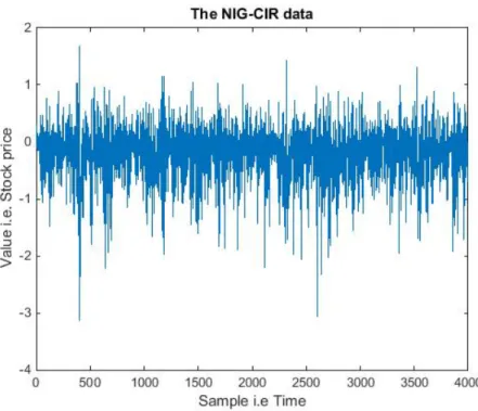
The parameter choices was influenced by parameters found in [3]. Generating the NIG-CIR data with these parameters yields the plots seen in Figure 1 and Figure 2 shows a closer look at the first 500 samples. This NIG-CIR data process is the one that is considered to be the true loss function and it is this one that the VaR and ES measurements are supposed to be calculated for using model averaging.
Figure 1: A plot over the data set used to estimate the parameters of the different processes. The first parameter set is used to generate the first 2000 samples and the remaining samples are generated using the second parameter set, seen on the previous page.
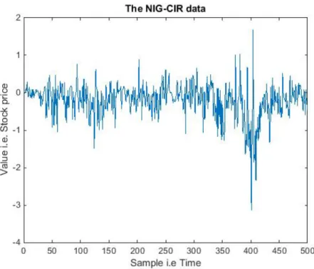
Figure 2: A closer look at the first 500 samples of the NIG-CIR data set. In this plot it is possible to see that the process have stochastic volatility.
3.2
Fitting distributions to the data
Once the data that was to be used as foundation for the simulations was gen-erated, the next step was to fit the different distributions to the data. The generated data set was 4000 samples long and for each fitting of parameter es-timates 1000 samples were used, iterating forward with 50 samples at a time finally yielding 60 parameter estimates for each distribution. The distributions that were fitted are:
• Normal Distribution
• Student’s t Distribution
• GARCH process with Normal Distribution
• GARCH process with Student’s t Distribution
• EGARCH with Normal Distribution
• Stochastic Volatility process - Taylor 82
Although six different distributions were fitted, only five were used in the pro-ceeding calculations. This is due to that the parameter estimates generated for the GARCH process with student’s t distribution sometimes yielded an unsta-ble processes. It is known from [14] that fitting staunsta-ble parameters to a GARCH process with student’s t distribution could be tricky and they have come up with a solution to this problem based on Generalized Auto regressive Scoring algorithms. But this article was found rather late in the process of this thesis and the method is hence not used in this thesis, instead the GARCH with Stu-dent’s t distribution is excluded when calculating the average. The interested reader can read more about the Generalized Autoregressive Scoring algorithms in [14].
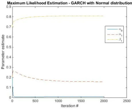
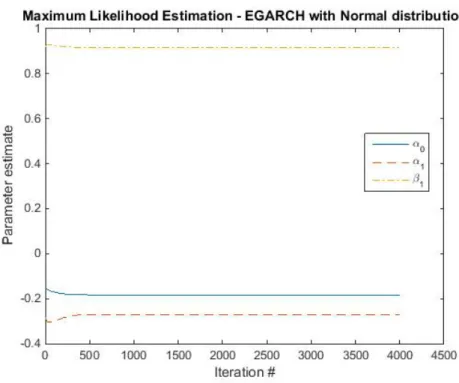
The Normal and Student’s t distribution were generated using the built in functions makedist and fitdist in Matlab. The fitting of the GARCH and EGARCH processes was done using MLE as explained in 2.6.2. To establish numerical stability and make sure that the estimator converged to the correct values, some tricks were performed. I.e. when taking the inverse of the Fisher matrix an eigenvalue matrix with small values were added to avoid zeros along the diagonal and the pseudo inverse, pinv, was used to calculate the inverse. And in order for the estimator not to take too big steps at each iteration, each step size was reduced and the number of iterations were increased to complement the reduced step size. In figure 3 and 4 the iteration process of the parameter estimates of the MLE procedure is showed.
Figure 3: The estimation of the parameters of the GARCH(1,1) with Normal distribution as the iteration proceeds
Figure 4: The estimation of the parameters of the EGARCH(1,1) as the iteration proceeds.
To calculate the parameters for the Taylor 82 process a Kalman filter was used.
Figure 5 to 9 shows the parameter estimates of the five different processes for the 60 different data sets. Comments on the different plots can be found in the captions.
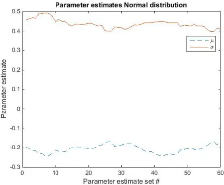
Figure 5: The parameter estimates of the Normal distribution for each of the 60 data sets. As seen the estimated parameters seem to be rather stable over the entire data set, even when the parameters have changed slightly it remains stable.
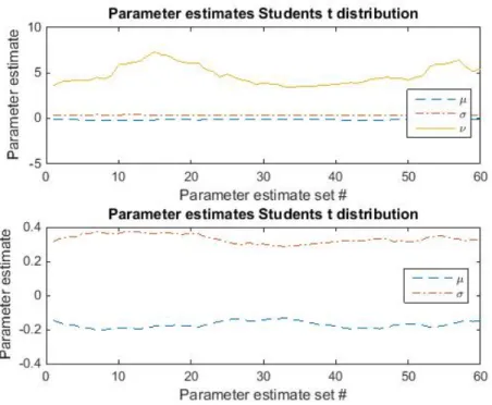
Figure 6: The parameter estimates of the Student’s t distribution for each of the 60 data sets. The most notable in this plot is how much the degrees of freedom,
ν changes. The reason for this is not something discussed closer in this thesis, but it is a behavior that is present rather often.
Figure 7: The parameter estimates of the GARCH(1,1) with Normal distribu-tion for each of the 60 data sets. The parameter estimates are rather consistent through out the plot and it is possible to see a small peak and dip in the esti-mates around sample no. 30. This is when there have been a slight change in the parameters generating the NIG-CIR process.
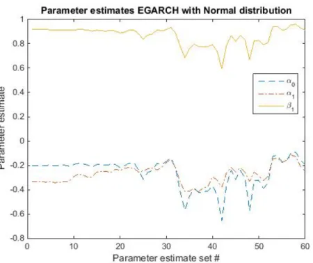
Figure 8: The parameter estimates of the EGARCH(1,1) distribution for each of the 60 data sets. The parameter estimates for the EGARCH process is not as stable for the second half of the data. Around 30 a clear dip is seen which is followed with more varying behavior. But it is possible to see that if there is a dip/peak in one of the estimated values, the other parameter estimates will also have a dip/peak at that time.
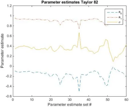
Figure 9: The parameter estimates of the Taylor 82 process for each of the 60 data sets. The parameter estimates for the Taylor 82 model show similarities to the EGARCH estimates in the sense that they are more stable in the first half, have a clear peak/dip around 30 and a more varying behavior in the second part.
3.3
BMA
The next step is to calculate weights used for the BMA. When calculating the weights BIC is used, the calculated BIC measures is of magnitude BIC ∼
1000−4000. If calculating the weights using (10) the magnitude of the BIC measure will become a problem, since the weights then become very large and approach infinity. Adjusting this as in (85) is the same thing as when using the unadjusted weights. This can be seen when normalizing the weights as in (86).
w=e(−BIC2 )=e(− BIC±A 2 )=e A 2e(− BIC−A 2 ) (85) Which yields wj= e(−BICj 2 ) Pn l=1e(− BICl 2 ) = e A 2e(− BICj−A 2 ) Pn l=1e A 2e(− BICl−A 2 ) = e (−BICj−A 2 ) Pn l=1e(− BICl−A 2 ) (86)
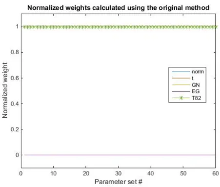
A problem with this way of calculating the weights is that due to the consider-ably different sizes of BIC only one of the models is considered, that is the Taylor 82 model which can be seen in 10. The way of calculating the log-Likelihood function have been validated by testing it on GARCH data, in which case the GARCH with Normal distribution and Taylor 82 model preforms equally well. The conclusion to draw from this is that considered the data in this thesis the Taylor 82 model is a significantly better fit than the other models, and hence it is the only one used.
But if instead adjusting the BIC according to (87)
w=e−(BIC2/A) (87)
all models get considered, even though the BIC values differs rather much. In both cases the constantAwas set to be BICmax which is the maximum BIC
from this set of values. Different choices of the value A was tested, i.e. the mean of the BIC values, but it was decided to use BICmaxsince it yielded good
results. The weights that were used was calculated according to (87) and can be seen in Figure 11. As seen in the figure this will yield a result that is rather close to equal weights. But with a slight consideration of the BIC measurements.
Figure 10: The calculated weights using the weight in (10). As seen in the figure only Taylor 82 is chosen.
Figure 11: The calculated weights using the weight in (87). All models will be considered almost equally, but the will be a preference of the Taylor 82, and a slight preference of the GARCH and EGARCH process.
Before finally calculating the BMA estimates for VaR and ES, the sample size used for the BMA need to be established. This was done according to (31), with the constantC= 10−2andα= 0.1 the sample sizeNαwas calculated to be
Nα=
1
0.1·(10−2)2 = 100 000 (88)
This means that using anα-level of 0.1 there will be∼10 000 samples that are used to calculate the ES estimate, which was deemed a sufficient amount of samples for the result to be relevant. Since VaR essentially is theα-quantile of the data, the matlab function prctile was used to calculate the VaR es-timates. When knowing the VaR estimates it is straight forward to calculate the ES estimates using (26). To be sure that the averaging of the VaR and ES estimates was not a problem the averaging was performed by creating a new mixed data sample, where the mixture was based on the weights. It was from this new weighted and mixed data sample the VaR and ES estimates finally were calculated.
4
Results
The calculated estimates for VaR and ES can be seen in Figure 12 to 15. It is the unconditional 1-step prediction of VaR and ES that is calculated. Due to that Monte Carlo methods is used to calculate VaR and ES, it is trivial to calculate the n-step prediction. As previously mentioned, when using the unadjusted weights only the Taylor 82 model is chosen is chosen, since it has the best fit for the data. That means that when it is written Taylor 82 in the figures, that correspond to the original weights and the parts where it is written weighted corresponds to the adjusted weights.
Figure 12: The different calculated VaR estimates. In the picture it is possible to see both the estimated values and the true value. One thing that is possible to see in this figure is that most of the functions under estimate the VaR, the idea was that GARCH with student’s t were to compensate for this, since the t distribution usually yields higher estimates, which also is possible to see in the picture.
Figure 13: A closer look at the more interesting VaR estimates, the different weighted averages, where the line corresponding to Taylor 82 also corresponds to the original weights.
Figure 15: A closer look at the more interesting ES estimates calculated using the different averaging processes. The line corresponding to Taylor 82 also corresponds to the original weights.
The first thing that is noticed when studying the different pictures is that there is not any average or model that outperforms the others, but they are all rather similar. One thing that is easy to see is that using only the Normal distribution will make for a underestimation of the risk. This is due to that the data has heavier tails than the Normal distribution is able to predict. Another thing that is seen in the figures is that the different estimates follow each other, if the one of the estimates increases in value, most of the others does the same at approximately the same time. A further interesting thing is that the EGARCH estimates yields an even worse estimate than the Normal distribution, the reason for this is unclear. In order to see if there seems to be any model that is performing better than the others the absolute value of the errors is analysed and the results are presented in the tables below.
Error of the Value-at-Risk estimates
Distribution Mean SD
Weighted average adjusted weights 0.6331 0.2741 Weighted average original weights 0.5641 0.2368 Equally weighted average 0.6320 0.2728 Normal distribution 1.0091 0.1569
Errors of the Expected Shortfall estimates
Distribution Mean SD
Weighted average adjusted weights 0.6324 0.2752 Weighted average original weights 0.6594 0.2802 Equally weighted average 0.6363 0.2803 Normal distribution 1.3041 0.2066
When studying the errors the previous guess that the different averaging estimates were similarly good is confirmed. Their mean errors are very similar to each other and they deviate approximately equally much from the true curve. It is known that an equally weighted portfolio sometimes outperforms a minimum variance portfolio when it is out of sample [16]. Considering the results in this thesis it is reasonable to assume that the same principle might be valid to this area of application.
There might be several reasons for these slightly vague results. One of these could be that there were some problems when fitting the different models to the unknown data, as it was with the GARCH with Student’s t distribution, so that the parameters did not converge to the optimal values. These problems could be due to the chosen parameters of the NIG-CIR process. Another problem is that the BIC values varied quite a lot, which lead to difficulties calculating the weights which in turn resulted in that solely the Taylor 82 process was chosen or that the averaging was performed with either equal or close to equal weights. Figure 16 shows a histogram of the NIG-CIR data used as validation of the estimates. The red line in the figure is a fitted Normal distribution. A closer
study of this figure shows that it has several of the properties that are common to financial data i.e. leptokurtosis, skewness and heavy tails. This is best seen by comparing to the Normal distribution in the picture. The peak is more narrow and higher than for the Normal distribution yielding that is it leptokurtic and the highest peak of the histogram is slightly shifted from that of the Normal distribution. By a closer study of the tails, it is possible to see that the NIG-CIR data has heavier tails than the Normal distribution. This explains why the VaR and ES estimates using only the Normal distribution is underestimated, as mentioned in 2.1.
Figure 16: A histogram of the NIG-CIR data, the red line corresponds to a Normal distribution fitted to the histogram.
5
Conclusions
As stated in the results, in this thesis, there is not one averaging process calcu-lating an average over several models or using one model, that fits remarkably better than the other. But calculating an average, regardless of the weights used, is extensively better than assuming that the data is Normal distributed. If the amount of time and work that is needed to calculate the different weights are taken into account when deciding on how good a fit the model is the con-clusion, based on the results in this thesis, is that the equally weighted average would be preferable over the weighted ones. This is due to that the accuracy of the estimates differ very little between the weighted and the equally weighted averages.
The main problem with the result in this thesis is that when using the intended weights, the fit of the Taylor 82 model was significantly better than for the other models to the extent where the Taylor 82 model was the only model chosen. If more models would have been considered it is likely that several of these would have given an equally good or even better fit than the Taylor 82 model. More models would also change the estimated weights which in turn might yield even better estimates.
And even though this thesis did not shine any light on which weights are the best to use to get the most accurate estimation fit, it is possible to draw the conclusion that using model averaging for calculating Value-at-Risk and Expected Shortfall is a good method. More considered models might also yield a more stable estimate.
A way to continue the research within this topic is to consider how to cal-culate the weights. There are many different information criterion’s that could be considered and that is just a small part all the possibilities for developing new weights. The interested reader can read more about different information criterions in [9].
Appendices
A
Derivation of the Hessian matrix - MLE
A.1 Normal distributionDeriving the expressions forJ originates from the log-Likelihood function. The log-likelihood function for the Normal distribution is seen in (89)
`Nt (θ) =−1 2log(2π)− 1 2log(σ 2 t)− 1 2 y2 σ2 t (89) The first derivative is
∂`Nt ∂θ = 1 2σ2 t ∂σt2 ∂θ yt2 σ2 t −1 (90) Yielding the second derivative to be
∂2`N t ∂θ∂θ = y2 t σ2 t −1 ∂ ∂θ 1 2σ2 t ∂σ2 t ∂θ ! + 1 2σ2 t ∂σ2 t ∂θ ∂ ∂θ y2 t σ2 t −1 = = y2 t σ2 t −1 ∂ ∂θ 1 2σ2 t ∂σ2 t ∂θ ! + y 2 t 2σ2 t ∂σ2 t ∂θ ∂(1/σ2 t) ∂σ2 t ∂σ2 t ∂θ = = yt2 σ2 t −1 ∂ ∂θ 1 2σ2 t ∂σ2t ∂θ ! − y 2 t 2(σ2 t) 3 ∂σt2 ∂θ ∂σt2 ∂θ (91)
Defining the standardized residuals asZt=yt/σtwhere Ztis SWN, so that
we haveZt|ψt−1∼SW N(0,1) [12]. The following results is known
E(Zt|ψt−1) = 0, E(Zt2|ψt−1) = 1, E(Zt2−1|ψt−1) = 0 (92)
Sinceσ2t only depends on past values of the residualsZi andσt2are
indepen-dent. Knowing this yields [12]
E Z 2 t (σ2 t) 2 ψt ! =E(Zt2)E 1 (σ2 t) 2 ! = 1 (σ2 t) 2 (93)
Combining the concept of standardized residuals with the expression in (91) yields the expression forJ
J =−E 1 2σ2 t (Zt2−1) ∂2σ2 t ∂θ∂θ − Z2 t 2(σ2 t) 2 ∂σ2 t ∂θ ∂σ2 t ∂θ ! =− 1 2σ2 t E(Zt2−1) ∂2σ2 t ∂θ∂θ + E(Z2 t) 2(σ2 t) 2 ∂σ2 t ∂θ ∂σ2 t ∂θ = 1 2σ4 t ∂σ2t ∂θ ∂σt2 ∂θ (94)
A.2 Student’s t distribution
The same calculations can be performed on the Student’s t distribution. Begin with the log-likelihhod function of the t distriution as seen in (95), the first derivative can then be seen in (96)
`Tt(θ) = log(Γ((ν+ 1)/2))−log(Γ(ν/2))−1 2log(π) −1 2log(ν−2)− 1 2log(σ 2 t)− ν+ 1 2 log 1 + y 2 (ν−2)σ2 t (95) ∂`Tt ∂θ = 1 2σ2 t ∂σt2 ∂θ yt2 σ2 t G −1 (96) WhereG is defined as in (97) G= ν+ 1 (ν−2) + yσ22 t (97) The second order derivative then becomes
∂2`T t ∂θ∂θ = y2 t σ2 t G −1 ∂ ∂θ 1 2σ2 t ∂σ2 t ∂θ ! + 1 2σ2 t ∂σ2 t ∂θ ∂ ∂θ y2 t σ2 t G −1 = = y2 t σt2 G −1 ∂ ∂θ 1 2σt2 ∂σ2 t ∂θ ! + y 2 t 2σt2 ∂σ2 t ∂θ ∂ ∂θ y2 t σt2 ν+ 1 (ν−2) +yσ22 t −1 ! = y2 t σ2 t G −1 ∂ ∂θ 1 2σ2 t ∂σt2 ∂θ ! − y 2 t 2σ2 t ∂σt2 ∂θ ∂σ2t ∂θ (ν+ 1)(ν−2) (σ2 t(ν−2) +yt2)2 (98) Using standardized residuals yields an expression forJ
J =−E 1 2σ2 t (Zt2 ν+ 1 (ν−2) +Z2 t −1)∂ 2σ2 t ∂θ∂θ− Zt2 2(σ2 t) 2 ∂σt2 ∂θ ∂σt2 ∂θ (ν+ 1)(ν−2) (ν−2)2+ 2(ν−2)Z2 t + (Zt2)2 ! =− 1 2σ2 t (E(Zt2) ν+ 1 (ν−2) +E(Z2 t) −1)∂ 2σ2 t ∂θ∂θ+ E(Zt2) 2(σ2 t) 2 ∂σ2t ∂θ ∂σ2t ∂θ (ν+ 1)(ν−2) (ν−2)2+ 2(ν−2)E(Z2 t) +E((Zt2)2) = 1 2(σ2 t) 2 (ν+ 1)(ν−2) ((ν−2) + 1)2 ∂σt2 ∂θ ∂σt2 ∂θ (99)
References
[1] Alexander J. McNeil, R¨udiger Frey, Paul Embrechts Qutantitative Risk Management, Princeton University press, Princeton, 2005.
[2] Martin Sk¨old Computer Intensive Statistical methods , Lund University, Lund, 2005.
[3] Andreas Kyprianou, Wim Schoutens, Paul WilmottExotic option pricing and advanced L´evy models, John Wiley & Sons Ldt., Chichester, 2005. [4] Andreas JakobssonTime Series Analysis and Signal modelling, Lund
Uni-versity, Lund, Edition 1:1, 2012.
[5] Erik Lindstr¨om, Henrik Madsen, Jan Nygaard Nielsen Statistics for Fi-nance, CRC Press, Boca Ranton, 2015.
[6] Christian Francq, Jean-Michel Zako¨ıanGARCH Models - structure, sta-tistical inference and financial applications , John Wiley & Sons Ldt., Chichester, 2010.
[7] Luc Bauwens, Christian Hafner, Sebastien LaurentHandbook of Volatility models and their applications, John Wiley & Sons Ldt., Chichester, 2012. [8] Nikolaus Hautsch, Yangguoyi OuDiscrete-Time Stochastic Volatility Mod-els and MCMC-Based Statistical Inference, SFB 649 Discussion Paper 2008-063, http://sfb649.wiwi.hu-berlin.de/papers/pdf/SFB649DP2008-063.pdf , 2008.
[9] Gerda Claeskens, Nils Lid HjorthModel Selection and Model Averaging, Cambridge University Press, Cambridge, 2008.
[10] Sadanori Konishi, Genshiro KitagawaInformation Criteria and Statistical modeling, Springer, New York, 2008.
[11] Jennifer A. Hoeting, David Madigan, Adrian E. Raftey, Chris T. Volinsky
Bayesian Model Averaging: A Tutorial, Statistical Science, Vol 14, No. 4, 1999 ,p. 382-417.
[12] George Levy Computational finance - numerical instruments for pricing financial instruments, Butterworth-Heinemann, Elsevier, Oxford, 2004. [13] R.I. Jennrich, P. F. Sampson Newton-Raphson and related Algorithms
for Maximum Likelihood Variance Component Estimation, Technometrics, 18:1, 1976 ,p. 11-17.
[14] Drew Creal, Siem Jan Koopman, Andr´e LucasGeneralized Autoregressive Score Models with applications, Journal of applied econometrics, 28, 2013 ,p. 777-795.
[15] Carol AlexanderMarket Risk Analysis Volume IV- Value-At-Risk Models, John Wiley & Sons Ltd, Chichester, 2008.
[16] Victor DeMiguel, Lorenzo Garlappi, Raman UppalOptimal Versus Naive Diversification: How Inefficient is the 1/N Portfolio Stratergy, Oxford University Press, Oxford, 2007.
Calculation of VaR and Expected Shortfall under
model uncertainty
Alexandra B¨ottern∗
∗Lund University
A common problem for financial institutions is to decide which model should be used when modelling prices and risks, in this article we focus on the risk aspect. When you have unknown data, for ex-ample losses, it is always a problem to decide which model to use when making the simulations, this is a concept called model risk. In this thesis the two risk measures calculated are Value-at-Risk and Expected Shortfall and they are calculated using a model averaging approach.
Value-at-Risk | Expected Shortfall | Bayesian Model Averaging
Value-at-Risk, or VaR as it is more commonly called, is a very common risk measurement used by financial institutions. It is often used to calculate market risk. Market risk is the risk of losses that a financial institution obtains due to factors affecting the financial market. An example of a market risk is that there might be a natural disaster or terrorist attack, this will affect the market as a whole. In Basel II, the second Basel accord, it is written that VaR is the preferred method for cal-culating market risk. But there are some problems with using VaR, for example it does not capture tail risk. And Value-at-Risk is not a coherent risk measure. This means that it does not fulfill the four axioms of coherence that follow below, the axiom it does not fulfill is the one for subadditivity.
1. Monotonicity- which can be explained as, if portfolio A is consistently better than portfolio B under almost all sce-narios then the risk of A should be less than the risk of B.
2. Subadditivity - meaning that the risk of portfolio A and B together cannot be worse than adding the risks for A and B separately.
3. Positive homogeneity - this means that if you double the size of your portfolio, you double the size of your risk. 4. Translation invariance- meaning that if you have one
port-folio A with a guaranteed return and a portport-folio B, the portfolio A is the same thing as adding cash to your port-folio B.
Since there is some problems with using VaR, the Basel committee have in Basel III decided that Expected Shortfall (ES) shall be used instead of VaR. Expected Shortfall is a risk measure that is closely related to Value-at-Risk, but it is
a coherent risk measure and it captures a lot of the behaviours that VaR does not.
Financial data often behaves in a special way and contain many complex behaviours. An example of this is that finan-cial data often is leptokurtic, meaning it have a more narrow and higher peak and heavier tails than the Normal distribu-tion. It is also common that it is skewed and that it contains volatility clustering. That a data series have volatility clus-ters means that one extreme event is likely to be followed by several extreme events.
These complex behaviours of financial data can be hard to model and predict if the underlying model is unknown, which usually is the case. In this thesis we use model aver-aging to solve this problem. By using model averaver-aging, or more specifically Bayesian Model Averaging, the model risk is reduced. This is due to that we now consider several mod-els instead of just choosing one. By choosing several modmod-els each one of them get to contribute with their unique behav-ior and generate a more confident final prediction. But there are some problems one is faced with when performing the av-eraging and one of these is how to select the weights used to calculate the average. We tried two different approaches when choosing the weights. One more naive approach using equal weights, which have proven to be rather good in the past. And one where the weights are calculated using Bayes Information Criterion (BIC). Bayes Information Criterion is a method of deciding which model is the best fit to the data using a Bayesian framework. The measurement is based on the log-likelihood function and punishes based on model com-plexity.
The different simulations performed shows that it is ad-vantageous to use BMA rather than using just one model. But due to some problems with the modelling the results are inconclusive regarding which weights are best to use. But if the time it took to calculate the weights is taken into consid-eration, the equally weighted average is to prefer since it is a lot faster to calculate and yielded an equally good result. Considering that Basel III states that Expected Shortfall is to be the recommended measurement to use when calculating market risk and that the BMA showed good results, I do be-lieve that this method is something that financial institutions can benefit from implementing.