A Two-Phase Augmented Lagrangian Method For Convex Composite Quadratic Programming

METHOD FOR CONVEX COMPOSITE

QUADRATIC PROGRAMMING

LI XUDONG

(B.Sc., University of Science and Technology of China)

A THESIS SUBMITTED

FOR THE DEGREE OF DOCTOR OF PHILOSOPHY

DEPARTMENT OF MATHEMATICS

NATIONAL UNIVERSITY OF SINGAPORE

2015

I hereby declare that the thesis is my original work and it has

been written by me in its entirety. I have duly acknowledged all

the sources of information which have been used in the thesis.

This thesis has also not been submitted for any degree in

any university previously.

Li, Xudong

21 January, 2015

I would like to express my sincerest thanks to my supervisor Professor Sun Defeng. Without his amazing depth of mathematical knowledge and professional guidance, this work would not have been possible. His mathematical programming module introduced me into the field of convex optimization, and thus, led me to where I am now. His integrity and enthusiasm for research has a huge impact on me. I owe him a great debt of gratitude.

My deepest gratitude also goes to Professor Toh Kim Chuan, my co-supervisor and my guide to numerical optimization and software. I have benefited a lot from many discussions we had during past three years. It is my great honor to have an opportunity of doing research with him.

My thanks also go to the previous and present members in the optimization group, in particular, Ding Chao, Miao Weimin, Jiang Kaifeng, Gong Zheng, Shi Dongjian, Wu Bin, Chen Caihua, Du Mengyu, Cui Ying, Yang Liuqing and Chen Liang. In particular, I would like to give my special thanks to Wu Bin, Du Mengyu, Cui Ying, Yang Liuqing, and Chen Liang for their enlightening suggestions and helpful discussions in many interesting optimization topics related to my research.

I would like to thank all my friends in Singapore at NUS, in particular, Cai Ruilun, Gao Rui, Gao Bing, Wang Kang, Jiang Kaifeng, Gong Zheng, Du Mengyu,

Ma Jiajun, Sun Xiang, Hou Likun, Li Shangru, for their friendship, the gatherings and chit-chats. I will cherish the memories of my time with them.

I am also grateful to the university and the department for providing me the four-year research scholarship to complete the degree, the financial support for conference trips, and the excellent research conditions.

Although they do not read English, I would like to dedicate this thesis to my parents for their unconditionally love and support. Last but not least, I am also greatly indebted to my fianc´ee, Chen Xi, for her understanding, encouragement and love.

Acknowledgements vii

Summary xi

1 Introduction 1

1.1 Motivations and related methods . . . 2

1.1.1 Convex quadratic semidefinite programming . . . 2

1.1.2 Convex quadratic programming . . . 8

1.2 Contributions . . . 11

1.3 Thesis organization . . . 13

2 Preliminaries 15 2.1 Notations . . . 15

2.2 The Moreau-Yosida regularization . . . 17

2.3 Proximal ADMM . . . 21

2.3.1 Semi-proximal ADMM . . . 22

2.3.2 A majorized ADMM with indefinite proximal terms . . . 27

3 PhaseI: A symmetric Gauss-Seidel based proximal ADMM for

con-vex composite quadratic programming 33

3.1 One cycle symmetric block Gauss-Seidel technique . . . 34

3.1.1 The two block case . . . 35

3.1.2 The multi-block case . . . 37

3.2 A symmetric Gauss-Seidel based semi-proximal ALM . . . 44

3.3 A symmetric Gauss-Seidel based proximal ADMM . . . 50

3.4 Numerical results and examples . . . 60

3.4.1 Convex quadratic semidefinite programming (QSDP) . . . 61

3.4.2 Nearest correlation matrix (NCM) approximations . . . 75

3.4.3 Convex quadratic programming (QP) . . . 79

4 Phase II: An inexact proximal augmented Lagrangian method for convex composite quadratic programming 89 4.1 A proximal augmented Lagrangian method of multipliers . . . 90

4.1.1 An inexact alternating minimization method for inner sub-problems . . . 96

4.2 The second stage of solving convex QSDP . . . 100

4.2.1 The second stage of solving convex QP . . . 107

4.3 Numerical results . . . 111

5 Conclusions 121

This thesis is concerned with an important class of high dimensional convex com-posite quadratic optimization problems with large numbers of linear equality and inequality constraints. The motivation for this work comes from recent interests in important convex quadratic conic programming problems, as well as from convex quadratic programming problems with dual block angular structures arising from network flows problems, two stage stochastic programming problems, etc. In order to solve the targeted problems to desired accuracy efficiently, we introduce a two phase augmented Lagrangian method, with Phase I to generate a reasonably good initial point and Phase II to obtain accurate solutions fast.

In Phase I, we carefully examine a class of convex composite quadratic program-ming problems and introduce a one cycle symmetric block Gauss-Seidel technique. This technique allows us to design a novel symmetric Gauss-Seidel based proximal ADMM (sGS-PADMM) for solving convex composite quadratic programming prob-lems. The ability of dealing with coupling quadratic term in the objective function makes the proposed algorithm very flexible in solving various multi-block convex optimization problems. The high efficiency of our proposed algorithm for achieving low to medium accuracy solutions is demonstrated by numerical experiments on various large scale examples including convex quadratic semidefinite programming

(QSDP) problems, convex quadratic programming (QP) problems and some other extensions.

In Phase II, in order to obtain more accurate solutions for convex composite quadratic programming problems, we propose an inexact proximal augmented La-grangian method (pALM). We study the global and local convergence of our posed algorithm based on the classic results of proximal point algorithms. We pro-pose to solve the inner subproblems by inexact alternating minimization method. Then, we specialize the proposed pALM algorithm to convex QSDP problems and convex QP problems. We discuss the implementation of a semismooth Newton-CG method and an inexact accelerated proximal gradient (APG) method for solving the resulted inner subproblems. We also show that how the aforementioned symmetric Gauss-Seidel technique can be intelligently incorporated in the implementation of our Phase II algorithm. Numerical experiments on a variety of high dimensional convex QSDP problems and convex QP problems show that our proposed two phase framework is very efficient and robust.

Chapter

1

Introduction

In this thesis, we focus on designing algorithms for solving large scale convex com-posite quadratic programming problems. In particular, we are interested in convex quadratic semidefinite programming (QSDP) problems and convex quadratic pro-gramming (QP) problems with large numbers of linear equality and inequality con-straints. The general convex composite quadratic optimization model we considered in this thesis is given as follows:

min ✓(y1) +f(y1, y2, . . . , yp) +'(z1) +g(z1, z2, . . . , zq)

s.t. A⇤

1y1+A⇤2y2+· · ·+A⇤pyp+B⇤1z1 +B2⇤z2+· · ·+B⇤qzq=c,

(1.1)

where p and q are given nonnegative integers, ✓ : _Y1 ! ( 1,+1] and ' : Z1 !

( 1,+1] are simple closed proper convex function in the sense that their proximal mappings are relatively easy to compute, f : _Y1 ⇥Y2 ⇥. . .⇥ Yp ! < and g :

Z1 ⇥Z2 ⇥. . .⇥Zq ! < are convex quadratic, possibly nonseparable, functions,

Ai : X ! Yi, i = 1, . . . , p, and Bj : X ! Zj, j = 1, . . . , q, are linear maps, c 2 X

is given data, Y1, . . . ,Yp,Z1, . . . ,Zq and X are real finite dimensional Euclidean

spaces each equipped with an inner product _h·,_·i and its induced norm_k·k.In this thesis, we aim to design efficient algorithms for finding a solution of medium to high accuracy to convex composite quadratic programming problems.

1.1

Motivations and related methods

The motivation for studying general convex composite quadratic programming model (1.1) comes from recent interests in the following convex composite quadratic conic programming problem: min ✓(y1) + 1 2hy1, Qy1i+hc, y1i s.t. y1 2K1, A⇤1y1 b2K2, (1.2)

where _Q : _Y1 ! Y1 is a self-adjoint positive semidefinite linear operator, c 2 Y1

and b _{2 X} are given data, _K1 ✓ Y1 and K2 ✓ X are closed convex cones. The

Lagrangian dual of problem (1.2) is given by max ✓⇤( s) 1

2hw, Qwi+hb, xi s.t. s+z Qw+A1x=c,

z 2K⇤

1, w2W, x2K⇤2,

where _{W ✓ Y}1 is any subspace such that Range(Q)✓ W, K⇤1 and K⇤2 are the dual

cones of K1 and K2, respectively, i.e., K⇤1 := {d 2 Y1 | hd, y1i 08y1 2 K1}, ✓⇤(·)

is the Fenchel conjugate function [53] of ✓(_·) defined by ✓⇤_{(s) = sup}

y12Y1{hs, y1i

✓(y1)}.

Below we introduce several prominent special cases of the model (1.2) including convex quadratic semidefinite programming problems and convex quadratic pro-gramming problems.

1.1.1

Convex quadratic semidefinite programming

An important special case of convex composite quadratic conic programming is the following convex quadratic semidefinite programming (QSDP)

min 1

2hX, QXi+hC, Xi

s.t. _AEX =bE, AIX bI, X 2S+n\K,

where Sn

+ is the cone of n⇥n symmetric and positive semidefinite matrices in the

space ofn_⇥nsymmetric matrices_Sn_{endowed with the standard trace inner product}

h·, ·i and the Frobenius norm k·k, Q is a self-adjoint positive semidefinite linear operator from _Sn _toSn_{, A}

E : Sn ! <mE and AI : Sn ! <mI are two linear maps,

C 2 Sn_{, b}

E 2 <mE and bI 2 <mI are given data, K is a nonempty simple closed

convex set, e.g.,_K=_{W _2Sn_{: LW U}withL, U 2S}n_{being given matrices.}

The dual of problem (1.3) is given by

max _K⇤( Z) 1₂hX0, QX0i+hbE, yEi+hbI, yIi s.t. Z QX0+S+A⇤ EyE +A⇤IyI =C, X0 2Sn_{, y} I 0, S 2S+n, (1.4)

where for any Z 2Sn_, ⇤

K( Z) is given by

⇤

K( Z) = _Winf_2KhZ, Wi= sup W2Kh

Z, W_i. (1.5)

Note that, in general, problem (1.4) does not fit our general convex composite quadratic programming model (1.1) unlessyI is vacuous from the model or K⌘Sn.

However, one can always reformulate problem (1.4) equivalently as min ( ⇤ K( Z) + <mI+ (u)) + 1 2hX0, QX0i+ Sn+(S) hbE, yEi hbI, yIi s.t. Z QX0_+S+A⇤ EyE +A⇤IyI =C, u yI = 0, X0 2Sn, (1.6) where _<mI

+ (·) is the indicator function over <

mI

+ , i.e., _<mI₊ (u) = 0 if u 2 <m+I and

<mI+ (u) =1 if u /2 <

mI

+ . Now, one can see that problem (1.6) satisfies our general

optimization model (1.1). Actually, the introduction of the variable u in (1.6) not only fits our model but also makes the computations more efficient. Specifically, in applications, the largest eigenvalue of AIA⇤I is normally very large. Thus, to

make the variable yI in (1.6) to be of free sign is critical for efficient numerical

computations.

Due to its wide applications and mathematical elegance [1, 26, 31, 50], QSDP has been extensively studied both theoretically and numerically in the literature. For the

recent theoretical developments, one may refer to [49, 61, 2] and references therein. From the numerical aspect, below we briefly review some of the methods available for solving QSDP problems. In (1.6), if there are no inequality constraints (i.e., AI and

bI are vacuous andK=Sn), Toh et al [63] and Toh [65] proposed inexact primal-dual

path-following methods, which belong to the category of interior point methods, to solve this special class of convex QSDP problems. In theory, these methods can be used to solve QSDP with any numbers of inequality constraints. However, in practice, as far as we know, the interior point based methods can only solve moderate scale QSDP problems. In her PhD thesis, Zhao [72] designed a semismooth Newton-CG augmented Lagrangian (NAL) method and analyzed its convergence for solving the primal formulation of QSDP problems (1.3). However, NAL algorithm may encounter numerical difficulty when the nonnegative constraints are present. Later, Jiang et al [29] proposed an inexact accelerated proximal gradient method mainly for least squares semidefinite programming without inequality constraints. Note that it is also designed to solve the primal formulation of QSDP. To the best of our knowledge, there are no existing methods which can efficiently solve the general QSDP model (1.3).

There are many convex optimization problems related to convex quadratic conic programming which fall within our general convex composite quadratic program-ming model. One example comes from the matrix completion with fixed basis coef-ficients [42, 41, 68]. Indeed the nuclear semi-norm penalized least squares model in [41] can be written as min X2<m⇥n 1 2kAFX dk 2_+⇢(kXk ⇤ hC, Xi) s.t. _AEX =bE, X2K:={X |kR⌦Xk1↵}, (1.7)

where kXk⇤ is the nuclear norm of X defined as the sum of all its singular values,

k·k1 is the element-wise l1 norm defined by kXk1 := max_i=1,...,mj=1max_,...,n|Xij|, AF :

<m⇥n _{! <}nF _and A

E : <m⇥n ! <nE are two linear maps, ⇢ and ↵ are two given

positive parameters, d _{2 <}nF_{, C 2 <}m⇥n _{and b}

E 2 <nE are given data, ⌦ ✓

are not fixed,R⌦ :<m⇥n ! <|⌦|is the linear map such thatR⌦X := (Xij)ij2⌦.Note

that when there are no fixed basis coefficients (i.e.,⌦=_{1, . . . , m_}⇥{1, . . . , n_}and AE are vacuous), the above problem reduces to the model considered by Negahban

and Wainwright in [45] and Klopp in [30]. By introducing slack variables ⌘, R and W, we can reformulate problem (1.7) as

min 1 2k⌘k 2_{+⇢ kRk} ⇤ hC, Xi + K(W) s.t. _AFX d=⌘, AEX =bE, X =R, X =W. (1.8)

The dual of problem (1.8) takes the form of

max _K⇤( Z) 1₂k⇠k2_{+hd, ⇠i+hb}

E, yEi

s.t. Z +A⇤

F⇠+S+A⇤EyE = ⇢C, kSk2 ⇢,

(1.9)

where _kS_k2 is the operator norm of S, which is defined to be its largest singular

value.

Another compelling example is the so called robust PCA (principle component analysis) considered in [66]: min _kA_k⇤+ 1kEk1+ 2 2kZk 2 F s.t. A+E+Z =W, A, E, Z _{2 <}m⇥n_, (1.10)

where W _{2 <}m⇥n _{is the observed data matrix, k·k}

1 is the elementwise l1 norm

given by _kE_k1 :=Pmi=1

Pn

j=1|Eij|, k·kF is the Frobenius norm, 1 and 2 are two

positive parameters. There are many di↵erent variants to the robust PCA model. For example, one may consider the following model where the observed data matrix W is incomplete: min _kA_k⇤+ 1kEk1+ 2 2 kP⌦(Z)k 2 F s.t. _P⌦(A+E+Z) = P⌦(W), A, E, Z 2 <m⇥n, (1.11)

i.e. one assumes that only a subset ⌦ _{✓ {}1, . . . , m_}⇥{1, . . . , n_} of the entries of W can be observed. HereP⌦:<m⇥n ! <m⇥n is the orthogonal projection operator

defined by P⌦(X) = 8 > < > : Xij if (i, j)2⌦, 0 otherwise. (1.12)

In [62], Tao and Yuan tested one of the equivalent forms of problem (1.11). In the numerical section, we will see other interesting examples.

Due to the fact that the objective functions in all above examples are separable, these examples can also be viewed as special cases of the following block-separable convex optimization problem:

minnXn i=1 i(wi)| Xn i=1H ⇤ iwi =c o , (1.13)

where for each i _{2 {}1, . . . , n_}, _Wi is a finite dimensional real Euclidean space

equipped with an inner producth·, ·iand its induced normk·k, i :Wi !( 1,+1]

is a closed proper convex function,_Hi :X !Wi is a linear map andc2X is given.

Note that the quadratic structure in all the mentioned examples is hidden in the sense that each i will be treated equally. However, this special quadratic structure

will be thoroughly exploited in our search for an efficient yet simple algorithm with guaranteed convergence.

Let >0 be a given parameter. The augmented Lagrangian function for (1.13) is defined by

L (w1, . . . , wn;x) :=P_in₌₁ i(wi) +hx, Pn_i=1H⇤iwi ci+ ₂kPn_i=1H⇤iwi ck2

for wi 2 Wi, i = 1, . . . , n and x 2 X. Choose any initial points w0i 2 dom( i),

i = 1, . . . , q and x0 _{2 X. The classical augmented Lagrangian method consists of}

the following iterations:

(w₁k+1, . . . , wk_n+1) = argminL (w1, . . . , wn;xk), (1.14) xk+1 = xk+⌧ ⇣Xn i=1H ⇤ iwki+1 c ⌘ , (1.15)

where ⌧ ₂ (0,2) guarantees the convergence. Due to the non-separability of the quadratic penalty term in L , it is generally a challenging task to solve the joint

minimization problem (1.14) exactly or approximately with high accuracy. To over-come this difficulty, one may consider the following n-block alternating direction methods of multipliers (ADMM):

w₁k+1 = argmin_L (w1, w2k. . . , wnk;xk), ... wk_i+1 = argmin_L (wk₁+1, . . . , wk_i+1₁, wi, wik+1, . . . , wnk;xk), ... (1.16) wk_n+1 = argmin_L (wk₁+1, . . . , wk_n+1₁, wn;xk), xk+1 _{= x}k_+⌧ ⇣Xn i=1H ⇤ iwik+1 c ⌘ .

Note that although the above n-block ADMM can not be directly applied to solve general convex composite quadratic programming problem (1.1) due to the nonsepa-rable structure of the objective functions, we still briefly discuss recent developments of this algorithm here as it is close related to our proposed new algorithm. In fact, the above n-block ADMM is an direct extension of the ADMM for solving the fol-lowing 2-block convex optimization problem

min_{ 1(w1) + 2(w2)| H1⇤w1+H⇤2w2 =c}. (1.17)

The convergence of 2-block ADMM has already been extensively studied in [18, 16, 17, 14, 15, 11] and references therein. However, the convergence of the n-block ADMM has been ambiguous for a long time. Fortunately this ambiguity has been addressed very recently in [4] where Chen, He, Ye, and Yuan showed that the direct extension of the ADMM to the case of a 3-block convex optimization problem is not necessarily convergent. This seems to suggest that one has to give up the direct extension of m-block (m 3) ADMM unless if one is willing to take a sufficiently small step-length ⌧ as was shown by Hong and Luo in [28] or to take a small penalty parameter if at least m 2 blocks in the objective are strongly convex [23, 5, 36, 37, 34]. On the other hand, the n-block ADMM with ⌧ 1 often

works very well in practice and this fact poses a big challenge if one attempts to develop new ADMM-type algorithms which have convergence guarantee but with competitive numerical efficiency and iteration simplicity as the n-block ADMM.

Recently, there is exciting progress in this active research area. Sun, Toh and Yang [59] proposed a convergent semi-proximal ADMM (ADMM+) for convex pro-gramming problems of three separable blocks in the objective function with the third part being linear. The convergence proof of ADMM+ presented in [59] is via establishing its equivalence to a particular case of the general 2-block semi-proximal ADMM considered in [13]. Later, Li, Sun and Toh [35] extended the 2-block semi-proximal ADMM in [13] to a majorized ADMM with indefinite semi-proximal terms. In this thesis, inspired by the aforementioned work, we aim to extend the idea in ADMM+ to solve convex composite quadratic programming problems based on the convergence results provided in [35].

1.1.2

Convex quadratic programming

As a special class of convex composite quadratic conic programming, the following high dimensional convex quadratic programming (QP) problem is also a strong motivation for us to study the general convex composite quadratic programming problem. The large scale convex quadratic programming with many equality and inequality constraints is given as follows:

min

⇢

1

2hx, Qxi+hc, xi|Ax=b, ¯b Bx2C, x2K , (1.18) where vector c_{2 <}n _{and positive semidefinite matrixQ 2S}n

+ define the linear and

quadratic costs for decision variable x 2 <n_{, matrices A 2 <}mE⇥n _{and B} 2 <mI⇥n

respectively define the equality and inequality constraints, _{C ✓ <}mI is a closed

convex cone, e.g., the nonnegative orthant _C = _{x¯ _{2 <}mI _{| x¯ 0}, K ✓ <}n _{is a}

being given vectors. The dual of (1.18) takes the following form

max ⇤

K( z) 12hx0, Qx0i+hb, yi+h¯b, y¯i

s.t. z Qx0_+A⇤_y+B⇤_{y¯=c, x}0 _{2 <}n_{, y¯2C ,}

(1.19)

where _C is the polar cone [53, Section 14] of _C. We are more interested in the case when the dimensions n and/ormE+mI are extremely large. Convex QP has been

extensively studied for over the last fifty years, see, for examples [60, 19, 20, 21, 8, 7, 9, 10, 70, 67] and references therein. Nowadays, main solvers for convex QP are based on active set methods or interior point methods. One may also refer tohttp://www. numerical.rl.ac.uk/people/nimg/qp/qp.html for more information. Currently, one popular state-of-the-art solver for large scale convex QP problems is the interior point methods based solver Gurobi[22]⇤. However, for high dimensional convex QP problems with a large number of constraints, the interior point methods based solvers, such as Gurobi, will encounter inherent numerical difficulties as the lack of sparsity of the linear systems to be solved often makes the critical sparse Cholesky factorization fail. This fact indicates that an algorithm which can handle high dimensional convex QP problems with many dense linear constraints is needed.

In order to handle the equality and inequality constraints simultaneously, we propose to add a slack variable ¯x to get the following problem:

min 1 2hx, Qxi+hc, xi s.t. 2 6 4 A B I 3 7 5 2 4 x ¯ x 3 5 = 2 4 b ¯ b 3 5, x2K, x¯2C. (1.20)

The dual of problem (1.20) is given by

max ( ⇤_K( z) _C⇤( ¯z)) 1₂hx0, Qx0i+hb, yi+h¯b, y¯i s.t. 2 4 z ¯ z 3 5 2 4 Qx0 0 3 5+ 2 4 A⇤ B⇤ I 3 5 2 4 y ¯ y 3 5 = 2 4 c 0 3 5. (1.21)

Thus, problem (1.21) belongs to our general optimization model (1.1). Note that, due to the extremely large problem size, ideally, one should decomposex0 _{into smaller}

pieces but then the quadratic term about x0 in the objective function becomes non-separable. Thus, one will encounter difficulties while using classic ADMM to solve (1.21) since classic ADMM can not handle nonseparable structures in the objective function. This again calls for new developments of efficient and convergent ADMM type methods.

A prominent example of convex QP comes from the two-stage stochastic opti-mization problem. Consider the following stochastic optiopti-mization problem:

min

x

n₁

2hx, Qxi+hc, xi+E⇠P(x;⇠)|Ax=b, x2K}, (1.22) where ⇠ is a random vector and

P(x;⇠) = min

⇢

1

2hx, Q¯ ⇠x¯i+hq⇠, x¯i|B⇠x¯= ¯b⇠ B⇠x, x¯2K⇠ ,

where _K⇠ 2X is a simple closed convex set depending on the random vector ⇠. By sampling N scenarios for ⇠, one may approximately solve (1.22) via the following deterministic optimization problem:

min 1₂hx, Qxi+hc, xi+PN_i=1(1₂hx¯i, Qix¯ii+hc¯i, x¯ii) s.t. 2 6 6 6 6 6 6 6 4 A B1 B1 ... . .. BN BN 3 7 7 7 7 7 7 7 5 2 6 6 6 6 6 6 4 x ¯ x1 ... ¯ xN 3 7 7 7 7 7 7 5 = 2 6 6 6 6 6 6 4 b ¯_b1 ... ¯_bN 3 7 7 7 7 7 7 5 , x2K, x¯= [¯x1;. . .; ¯xN]2K=K1⇥· · ·⇥KN, (1.23)

where Qi =piQi and ¯ci =piqi with pi being the probability of occurrence of theith

with the ith scenario. The dual problem of (1.23) is given by min (PN_j=1 ⇤ Kj( zj) + K⇤( z)) + 1 2hx0, Qx0i+ PN i=1 1 2hx¯0i, Qix¯0ii hb, yi PN j=1h¯bj,y¯ji s.t. 2 6 6 6 6 6 6 4 z ¯ z1 .. . ¯ zN 3 7 7 7 7 7 7 5 2 6 6 6 6 6 6 4 Q Q1 . .. QN 3 7 7 7 7 7 7 5 2 6 6 6 6 6 6 4 x0 ¯ x0 1 .. . ¯ x0N 3 7 7 7 7 7 7 5 + 2 6 6 6 6 6 6 4 A⇤ _B⇤ 1 · · · B⇤N B⇤1 . .. B⇤N 3 7 7 7 7 7 7 5 2 6 6 6 6 6 6 4 y ¯ y1 .. . ¯ yN 3 7 7 7 7 7 7 5 = 2 6 6 6 6 6 6 4 c ¯ c1 .. . ¯ cN 3 7 7 7 7 7 7 5 . (1.24)

Clearly, (1.24) is another perfect example of our general convex composite quadratic programming problems.

1.2

Contributions

In order to solve the convex composite quadratic programming problems (1.1) to high accuracy efficiently, we introduce a two-phase augmented Lagrangian method, with Phase I to generate a reasonably good initial point and Phase II to obtain ac-curate solutions fast. In fact, this two stage framework has been successfully applied to solve semidefinite programming (SDP) problems with partial or full nonnegative constraints where ADMM+ [59] and SDPNAL+ [69] are regraded as Phase I algo-rithm and Phase II algoalgo-rithm, respectively. Inspired by the aforementioned work, we propose to extend their ideas to solve large scale convex composite quadratic programming problems including convex QSDP and convex QP.

In Phase I, to solve convex quadratic conic programming, the first question we need to ask is that shall we work on the primal formulation (1.2) or the dual for-mulation (1.3)? Note that since the objective function in the dual problem contains quadratic functions as the primal problem does and has more blocks, it is natural for people to focus more on primal formulation. Actually, the primal approach has been used to solve special class of QSDP as in [29, 72]. However, as demonstrated in [59, 69], it is usually better to work on the dual formulation than the primal formulation for linear SDP problems with nonegative constraints (SDP+). [59, 69] pose the following question: for general convex quadratic conic programming (1.2),

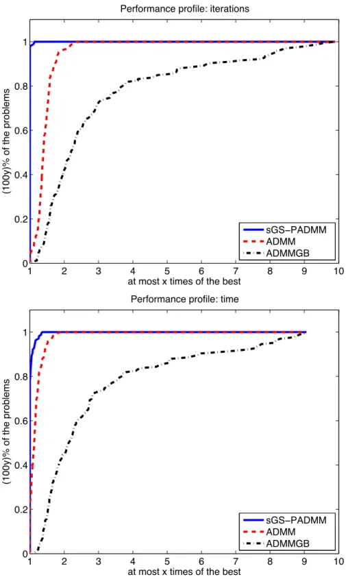
can we work on the dual formulation instead of primal formulation, as for the lin-ear SDP+ problems? So that when the quadratic term in the objective function of QSDP reduced to a linear term, our algorithm is at least comparable with the algorithms proposed [59, 69]. In this thesis, we will resolve this issue in a unified way elegantly. Observe that ADMM+ can only deal with convex programming problems of three separable blocks in the objective function with the third part being lin-ear. Thus, we need to invent new techniques to handle the quadratic terms and the multi-block structure in (1.4). Fortunately, by carefully examining a class of convex composite quadratic programming problems, we are able to design a novel one cy-cle symmetric block Gauss-Seidel technique to deal with the nonseparable structure in the objective function. Based on this technique, we then propose a symmetric Gauss-Seidel based proximal ADMM (sGS-PADMM) for solving not only the dual formulation of convex quadratic conic programming, which includes the dual formu-lation of QSDP as a special case, but also the general convex composite quadratic optimization model (1.1). Specifically, when sGS-PADMM is applied to solve high dimensional convex QP problems, the obstacles brought about by the large scale quadratic term, linear equality and inequality constraints can thus be overcome via using sGS-PADMM to decompose these terms into smaller pieces. Extensive nu-merical experiments on high dimensional QSDP problems, convex QP problems and some extensions demonstrate the efficiency of sGS-PADMM for finding a solution of low to medium accuracy.

In Phase I, the success of sGS-PADMM of being able to decompose the non-separable structure in the dual formulation of convex quadratic conic programming (1.3) depends on the assumptions that the subspace _W in (1.3) is chosen to be the whole space. This in fact can introduce unfavorable property of the unbounded-ness of the dual solution w to problem (1.3). Fortunately, it causes no problem in Phase I. However, this unboundedness becomes critical in designing our second phase algorithm. Therefore, in Phase II, we will take _W = Range(_Q) to eliminate the unboundedness of the dual optimal solution w. This of course will introduce

numerical difficulties as we need to maintain w 2 Range(Q), which, in general, is a difficult task. However, by fully exploring the structure of problem (1.3), we are able to resolve this issue. In this way, we can design an inexact proximal augmented Lagrangian (pALM) method for solving convex composite quadratic programming. The global convergence is analyzed based on the classic results of proximal point algorithms. Under the error bound assumption, we are also able to establish the local linear convergence of our proposed algorithm pALM. Then, we specialize the proposed pALM algorithm to convex QSDP problems and convex QP problems. We discuss in detail the implementation of a semismooth Newton-CG method and an inexact accelerated proximal gradient (APG) method for solving the resulted inner subproblems. We also show that how the aforementioned symmetric Gauss-Seidel technique can be intelligently incorporated in the implementation of our Phase II algorithm. The efficiency and robustness of our proposed two phase framework is then demonstrated by numerical experiments on a variety of high dimensional convex QSDP and convex QP problems.

1.3

Thesis organization

The rest of the thesis is organized as follows. In Chapter 2, we present some pre-liminaries that are relate to the subsequent discussions. We analyze the property of the Moreau-Yosida regularization and review the recent developments of proximal ADMM. In Chapter 3, we introduce the one cycle symmetric block Gauss-Seidel technique. Based on this technique, we are able to present our first phase algo-rithm, i.e., a symmetric Gauss-Seidel based proximal ADMM (sGS-PADMM), for solving convex composite quadratic programming problems. The efficiency of our proposed algorithm for finding a solution of low to medium accuracy to the tested problems is demonstrated by numerical experiments on various examples including convex QSDP and convex QP. In Chapter 4, for Phase II, we propose an inexact proximal augmented Lagrangian method for solving our convex composite quadratic

optimization model and analyze its global and local convergence. The inner subprob-lems are solved by an inexact alternating minimization method. We also discuss in detail the implementations of our proposed algorithm for convex QSDP and convex QP problems. We also show that how the aforementioned symmetric Gauss-Seidel technique can be wisely incorporated in the proposed algorithms for solving the re-sulted inner subproblems. Numerical experiments conducted on a variety of large scale convex QSDP and convex QP problems show that our two phase framework is very efficient and robust for finding high accuracy solutions for convex composite quadratic programming problems. We give the final conclusions of the thesis and discuss a few future research directions in Chapter 5.

Chapter

2

Preliminaries

2.1

Notations

Let X and Y be finite dimensional real Euclidian spaces each equipped with an inner product _h·,_·i and its induced norm _k·k. Let _M : _{X ! X} be a self-adjoint positive semidefinite linear operator. Then, there exists a unique positive semidef-inite linear operator _N with _N2 _{= M. Thus, we define M}1_{2 =} p_{M = N.}

Define h·, ·iM : X ⇥ X ! < by hx, yiM = hx, Myi for all x, y 2 X. Let

k· kM : X ! < be defined as kxkM =

p

hx, x_iM for all x _{2 X}. If, _M is fur-ther assumed to be positive definite, h·, ·iM will be an inner product and k·kM

will be its induced norm. Let _Sn

+ be the cone of n ⇥ n symmetric and

posi-tive semidefinite matrices in the space of n ⇥n symmetric matrices Sn _endowed

with the standard trace inner product _h·,_·i and the Frobenius norm _{k ·k}. Let

svec:Sn_{! <}n(n+1)/2 _{be the vectorization operator on symmetric matrices defined}

by svec(X) := [X11, p 2X12, X22, . . . , p 2X1n, . . . , p 2Xn 1,n, Xnn]T.

Definition 2.1. A function F : X ! Y is said to be directionally di↵erentiable at

x_2X if

F0(x;h) := lim

t!0+

F(x+th) F(x)

t exists

for all h2X and F is directionally di↵erentiable if F is directionally di↵erentiable

at every x2X.

Let F : _{X ! Y} be a Lipschitz continuous function. By Rademacher’s theorem [56, Section 9.J],F is Fr´echet di↵erentiable almost everywhere. LetDF be the set of

points in _X where F is di↵erentiable. The Bouligand subdi↵erential of F at x_2X is defined by @BF(x) = ⇢ lim xk_!xF 0_(xk_{), x}k 2DF ,

whereF0_(xk_{) denotes the Jacobian ofF atx}k _2D

F and the Clarke’s [6] generalized

Jacobian of F at x2X is defined as the convex hull of @BF(x) as follows

@F(x) = conv_{@BF(x)}.

First introduced by Miffin [43] for functionals, the following concept of semismooth-ness was then extended by Qi and Sun [51] to cases when a vector-valued function is not di↵erentiable, but locally Lipschitz continuous. See also [12, 40]

Definition 2.2. LetF :_{O ✓X !Y} be a locally Lipschitz continuous function on

the open set O. F is said to be semismooth at a point x2O if 1. F is directionally di↵erentiable at x; and

2. for any x_2X and V ₂@F(x+ x) with x_!0, F(x+ x) F(x) V x=o(k xk).

Furthermore,F is said to be strongly semismooth atx_2X ifF is semismooth at xand for any x2X and V 2@F(x+ x) with x!0,

F(x+ x) F(x) V x=O(_k x_k2).

In fact, many functions such as convex functions and smooth functions are semis-mooth everywhere. Moreover, piecewise linear functions and twice continuously di↵erentiable functions are strongly semismooth functions.

2.2

The Moreau-Yosida regularization

In this section, we discuss the Moreau-Yosida regularization which is a useful tool in our subsequent analysis.

Definition 2.3. Let f : X ! ( 1,1] be a closed proper convex function. Let

M:_{X !X} be a self-adjoint positive definite linear operator. The Moreau-Yosida regularization 'f_M :X ! < of f with respect to Mis defined as

'f_M(x) = min z2X ⇢ f(z) + 1 2kz xk 2 M , x2X. (2.1)

From [44, 71], we have the following proposition.

Proposition 2.1. For any given x 2 X, the problem (2.1) has a unique optimal

solution.

Definition 2.4. The unique optimal solution of problem (2.1), denoted by proxf_M(x),

is called the proximal point ofxassociated withf. When_M=_I, for simplicity, we write prox_f(x)⌘proxf_I(x) for all x2X, where I :X !X is the identity operator. Below, we list some important properties of the Moreau-Yosida regularization.

Proposition 2.2. Let g :X !( 1,+1] be defined as g(x)⌘f(M 12x)8x2X.

Then,

proxf_M(x) =M 12prox

g(M

1

2x) 8x2X.

Proof. Note that, for any given x2X,

proxf_M(x) = argmin_{f(z) + 1 2kz xk 2 M} = argmin{f(z) + 1 2kM 1 2z M 1 2xk2}.

By change of variables, we have proxf_M(x) =_M 12y, where

y = argmin{f(M 12y) + 1 2ky M 1 2xk2}= argmin{g(y) + 1 2ky M 1 2xk2} = prox_g(_M12x).

That is proxf_M(x) =M 12proxg

I(M

1

Proposition 2.3. [32, Theorem XV.4.1.4 and Theorem XV.4.1.7] Let f : X ! ( ₁,+₁] be a closed proper convex function. Let _M : _{X ! X} be a given self-adjoint positive definite linear operator, 'f_M(x) be the Moreau-Yosida regularization of f, and proxf_M : _{X !X} be the associated proximal mapping. Then the following properties hold.

(i) argminx2Xf(x) = argminx2X'fM(x).

(ii) Both proxf_M andQf_M :=I proxf_M (I :X !X is the identity map) are firmly non-expensive, i.e., for any x, y _2X,

kproxf_M(x) proxf_M(y)k2

M  hproxfM(x) prox f

M(y), x yiM, (2.2)

kQf_M(x) Qf_M(y)_k2_{M  h}Qf_M(x) Qf_M(y), x y_iM. (2.3) (iii) 'f_M is continuous di↵erentiable, and further more, it holds that

r'f_M(x) =_M(x proxf_M(x))₂@f(proxf_M(x)). Hence,

f(v) f(proxf_M(x)) +_hx proxf_M(x), v proxf_M(x)_{iM 8}v _2X.

Proposition 2.4 (Moreau Decomposition). Let f :X !( 1,+1]be a closed

proper convex function and f⇤ _{be its conjugate. Then any z 2 X has the}

decompo-sition

z= proxf_M(z) +_M 1proxf_M⇤ 1(Mz).

Proof: For any given z _2X, by definition of proxf_M(z), we have

02@f(proxf_M(z)) +M(proxf_M(z) z), i.e., z proxf_M(z) _{2 M} 1_@f(proxf

M(z)). Define function g : X ! ( 1,+1] as

g(x) ⌘f(M 1_{x). By [53, Theorem 9.5], g is also a closed proper convex function.}

By [53, Theorem 12.3 and Theorem 23.9], we have

respectively. Thus, we obtain

z proxf_M(z)₂@g(_Mproxf_M(z)).

Then, by [53, Theorem 23.5 and Theorem 23.9], it is easy to have that Mproxf_M(z)2@g⇤(z proxf_M(z)) =M@f⇤ M(z proxf_M(z)) . Therefore, M(z proxf_M(z)) = argmin_y2X ⇢ f⇤(y) + 1 2ky Mzk 2 M 1 = proxf_M⇤ 1(Mz).

Thus, we complete the proof.

Now let us consider a special application of the aforementioned Moreau-Yosida regularization.

We first focus on the case where the function f is assumed to be the indicator function of a given closed convex set _K, i.e.,f(x) = _K(x) where _K(x) = 0 ifx_2K and _K(x) = 1if x /2K. For simplicity, we also let the self-adjoint positive definite linear operator _M to be the identity operator _I. Then, the proximal point of x associated with indicator function f(·) = _K(·) with M =I is the unique optimal solution, denoted by ⇧_K(x), of the following convex optimization problem:

min 1

2kz xk

2

s.t. z 2K.

(2.4)

In fact, ⇧_K : _{X ! X} is the metric projector over _K. Thus, the distance function is defined by dist(x,K) = kx ⇧_K(x)k. By Proposition 2.3, we know that ⇧_K(x) is Lipschitz continuous with modulus 1. Hence, ⇧_K(_·) is almost everywhere Fr´echet di↵erentiable in X and for every x 2X, @⇧_K(x) is well defined. Below, we list the following lemma [40], which provides some important properties of @⇧_K(_·).

Lemma 2.5. Let _{K ✓ X} be a closed convex set. Then, for any x _{2 X} and _{V 2}

1. V is self-adjoint. 2. hh, Vhi 0 8h2X. 3. _hh, _Vh_{i kV}h_k2 _8h2X.

Let _K = _{W _{2 S}n _{| L  W  U} with L, U 2 S}n _{being given matrices. For}

X 2 Sn_{, let Y = ⇧}

K(X) be the metric projection of X onto the subset K of Sn

under the Frobenius norm. Then, Y = min(max(X, L), U). Define linear operator W0 _:Sn_!Sn _by W0(M) = ⌦ M, M _2Sn, where ⌦ij = 8 > > > < > > > : 0 if Xij < Lij, 1 if Lij Xij Uij, 0 if Xij > Uij. (2.5)

Observing that ⇧_K(X) now is in fact a piecewise linear function, we have W0 _{is an}

element of the set @⇧_K(X). LetK=Sn

+, i.e., the cone ofn⇥n symmetric and positive semidefinite matrices.

GivenX _2Sn_{, letX}

+ =⇧Sn

+(X) be the projection ofXontoS

n

+under the Frobenius

norm. Assume that X has the following spectral decomposition X =P⇤PT,

where ⇤ is the diagonal matrix with diagonal entries consisting of the eigenvalues

1 2 · · · k > 0 k+1 . . . n of X and P is a corresponding

orthogonal matrix of eigenvectors. Then

X+=P⇤+PT,

where ⇤+ = max{⇤,0}. Sun and Sun, in their paper [58], show that ⇧Sn

+(·) is

strongly semismooth everywhere in Sn_{. Define the operator W}0 _:Sn _!Sn _by

where ⌦= 0 @ Ek ⌦ ⌦T 0 1 A, ⌦ij = i i j , i_2{1, . . . , k_}, j _2{k+ 1, . . . , n_},

where Ek is the square matrix of ones with dimension k (the number of positive

eigenvalues), and the matrix ⌦has all its entries lying in the interval [0,1]. In their paper [47], Pang, Sun and Sun proved that W0 _{is an element of the set@⇧}

Sn

+(X).

Next we examine the case when the functionf is chosen as follows: f(x) = _K⇤( x) = inf

z2Khz, xi= supz2Kh

z, x_i, (2.7)

where Kis a given closed convex set. Then, by Proportion 2.3 and Proposition 2.4, we have the following useful results.

Proposition 2.6. Let '(¯x) := min ⇤_K( x) +

2kx x¯k

2_{, the following results hold:}

(i) x+ _{= argmin} ⇤ K( x) + ₂kx x¯k2 = ¯x+ 1 ⇧_K( x¯). (ii) r'(¯x) = (¯x x+_{) = ⇧} K( x¯). (iii) '(¯x) = h x+, ⇧_K( x¯)i+ 1 2 k⇧K( x¯)k 2 _{= hx,¯ ⇧} K( x¯)i 1 2 k⇧K( x¯)k 2_.

2.3

Proximal ADMM

In this section, we review the convergence results for the proximal alternating direc-tion method of multipliers (ADMM) which will be used in our subsequent analysis. Let X, Y and Z be finite dimensional real Euclidian spaces. Let F : Y ! ( ₁,+₁] and G:_{Z !}( ₁,+₁] be closed proper convex functions, _F :_{X !Y} andG :X !Z be linear maps. Let@F and@Gbe the subdi↵erential mappings ofF and G, respectively. Since both @F and @G are maximally monotone [56, Theorem 12.17], there exist two self-adjoint and positive semidefinite operators ⌃F and ⌃G

[13] such that for all y,y˜₂dom(F), ⇠₂@F(y), and ˜⇠ ₂@F(˜y), h⇠ ⇠˜, y y˜i ky y˜k2

and for all z,z˜2dom(G), ⇣ 2@G(z), and ˜⇣ 2@G(˜z),

h⇣ ⇣˜, z z˜_{i k}z z˜_k2_⌃G. (2.9)

2.3.1

Semi-proximal ADMM

Firstly, we discuss the semi-proximal ADMM proposed in [13]. Consider the convex optimization problem with the following 2-block separable structure

min F(y) +G(z) s.t. _F⇤_y+G⇤_z=c.

(2.10)

The dual of problem (2.10) is given by

min_{hc, x_i+F⇤(s) +G⇤(t)_{| F}x+s= 0, _Gx+t= 0_}. (2.11) Let >0 be given. The augmented Lagrangian function associated with (2.10) is given as follows:

L (y, z;x) = F(y) +G(z) +hx, F⇤_y+G⇤_{z ci+}

2kF

⇤_y+G⇤_{z ck}2_.

The semi-proximal ADMM proposed in [13], when applied to (2.10), has the following template. Since the proximal terms added here are allowed to be posi-tive semidefinite, the corresponding method is referred to as semi-proximal ADMM instead of proximal ADMM as in [13].

Algorithm sPADMM: A generic 2-block semi-proximal ADMM for solv-ing (2.10).

Let >0 and⌧ ₂(0,₁) be given parameters. Let _TF and TG be given self-adjoint

positive semidefinite, not necessarily positive definite, linear operators defined on Y and _Z, respectively. Choose (y0_{, z}0_{, x}0_{)2dom(F)⇥dom(G)⇥X.Fork = 0,1,2, ...,}

perform the kth iteration as follows:

Step 1. Compute yk+1 = argmin_y L (y, zk;xk) + 2ky y k_k2 TF. (2.12) Step 2. Compute zk+1 = argmin_{z L} (yk+1, z;xk) + 2kz z k k2TG. (2.13) Step 3. Compute xk+1 _=xk_{+⌧ (F}⇤_yk+1_+G⇤_zk+1 _{c). (2.14)}

In the above 2-block semi-proximal ADMM for solving (2.10), the presence ofTF

and _TG can help to guarantee the existence of solutions for the subproblems (2.12)

and (2.13). In addition, they play important roles in ensuring the boundedness of the two generated sequences _{yk+1_{} and {z}k+1_{}. Hence, these two proximal terms}

are preferred. The choices of TF and TG are very much problem dependent. The

general principle is that both _TF and TG should be as small as possible while yk+1

and zk+1 _{are still relatively easy to compute.}

For the convergence of the 2-block semi-proximal ADMM, we need the following assumption.

Assumption 1. There exists (ˆy,zˆ)2ri(domF ⇥domG) such that F⇤_yˆ+G⇤_zˆ=c.

Theorem 2.7. Let ⌃F and ⌃G be the self-adjoint and positive semidefinite

(2.10)is nonempty and that Assumption 1 holds. Assume that TF andTGare chosen

such that the sequence _{(yk_{, z}k_{, x}k_{)} generated by Algorithm sPADMM is well}

de-fined. Then, under the condition either (a)⌧ 2(0,(1+p5 )/2)or (b)⌧ (1+p5 )/2

but P1_k=0(_kG⇤_(zk+1 _zk_)k2_+⌧ 1_kF⇤_yk+1_+G⇤_zk+1 _ck2_{)<1, the following results}

hold:

(i) If(y1_{, z}1_{, x}1_{)is an accumulation point of{(y}k_{, z}k_{, x}k_{)}, then(y}1_{, z}1_)solves

problem (2.10) and x1 _{solves (2.11), respectively.}

(ii) If both 1_⌃

F +TF +FF⇤ and 1⌃G+TG+GG⇤ are positive definite, then

the sequence _{(yk_{, z}k_{, x}k_{)}, which is automatically well defined, converges to a}

unique limit, say, (y1_{, z}1_{, x}1_{) with (y}1_{, z}1_{) solving problem (2.10) and x}1

solving (2.11), respectively.

(iii) When the y-part disappears, the corresponding results in parts (i)–(ii) hold under the condition either ⌧ ₂(0,2) or ⌧ 2 but P_k1_=0kG⇤_zk+1 _ck2 _<1.

Remark 2.8. The conclusions of Theorem 2.7 follow essentially from the results

given in [13, Theorem B.1]. See [59] for more detailed discussions.

As a simple application of the aforementioned semi-proximal ADMM algorithm, we present a special semi-proximal augmented Lagrangian method for solving the following block-separable convex optimization problem

min PN_i=1✓i(vi)

s.t. PN_i=1A⇤

ivi =c,

(2.15)

where N is a given positive integer, ✓i : Vi ! ( 1,+1], i = 1, . . . , N are

closed proper convex functions, _Ai : X ! Vi, i = 1, . . . , N are linear operators,

V1, . . . ,VN are all real finite dimensional Euclidean spaces each equipped with an

V := V1 ⇥ V2⇥, . . . ,VN. For any v 2 V, we write v ⌘ (v1, v2, . . . , vN) 2 V.

De-fine the linear map _A :_{X !V} such that its adjoint is given by A⇤v = N X i=1 A⇤ivi 8v 2V. Additionally, let ✓(v) = N X i=1 ✓i(vi) 8v 2V.

Given > 0, the augmented Lagrange function associated with (2.15) is given as follows:

L✓_{(v;x) = ✓(v) +hx, A}⇤_{v ci+}

2kA

⇤_{v ck}2_{. (2.16)}

In order to handle the non-separability of the quadratic penalty term in _L✓_{, as well} as to design efficient parallel algorithm for solving problem (2.15), we propose the following novel majorization step

AA⇤ ₌ 0 B B B @ A1A⇤1 · · · A1A⇤N ... . .. ... ANA⇤1 . . . ANA⇤N 1 C C C A (2.17) M:= Diag(_M1, . . . ,MN), with _Mi ⌫ AiA⇤i + P j6=i(AiA⇤jAjA⇤i) 1

2. Let S : Y ! Y be a self-adjoint linear

operator given by

S :=M AA⇤_{. (2.18)}

Here, we state a useful proposition to show that _S is indeed a self-adjoint positive semidefinite linear operator.

Proposition 2.9. It holds that S =M AA⇤ _⌫0.

Proof. The proposition can be proved by observing that for any given matrix

X 2 <m⇥n_{, it holds that} 0 @ X X⇤ 1 A 0 @ (XX⇤) 1 2 (X⇤X)12 1 A.

Define T✓ : V ! V to be a self-adjoint positive semidefinite, not necessarily positive definite, linear operator given by

T✓ := Diag(T✓1, . . . ,T✓N), (2.19)

where fori= 1, . . . , N, each_T✓i is a self-adjoint positive semidefinite linear operator

defined onViand is chosen such that the subproblem (2.20) is relatively easy to solve.

Now, we are ready to propose a semi-proximal augmented Lagrangian method with a Jacobi type decomposition for solving (2.15).

Algorithm sPALMJ: A semi-proximal augmented Lagrangian method with a Jacobi type decomposition for solving (2.15).

Let >0 and⌧ 2(0,1) be given initial parameters. Choose (v0_{, x}0_{)2dom(✓)⇥X.}

For k= 0,1,2, ..., generate vk+1 _{according to the following iteration:}

Step 1. Fori= 1, . . . , N, compute

v_ik+1 = argmin_vi 8 < : L✓_((vk 1, . . . , vik 1, vi, vik+1, . . . , vNk);xk) +₂kvi vikk2Mi AiiA⇤ii + 2kvi v k ik2T✓_i 9 = ;. (2.20) Step 2. Compute xk+1 =xk+⌧ (_A⇤vk+1 c). (2.21)

The relationship between Algorithm sPALMJ and Algorithm sPADMM for solv-ing (2.15) will be revealed in the next proposition. Hence, the convergence of Algo-rithm sPALMJ can be easily obtained under certain conditions.

Proposition 2.10. For any k 0, the point (vk+1_{, x}k+1_{) obtained by Algorithm}

sPALMJ for solving problem (2.15)can be generated exactly according to the follow-ing iteration: vk+1= argmin_{v L}✓(v;xk) + 2kv v k k2S+ ₂kv vkk2T✓. xk+1 =xk+⌧ (_A⇤vk+1 c).

Proof. The equivalence can be obtained by carefully examining the optimality conditions for subproblems (2.20) in Algorithm sPALMJ.

2.3.2

A majorized ADMM with indefinite proximal terms

F(y) = p(y) +f(y) and G(z) = q(z) +g(z),

where p : _{Y !} ( ₁,+₁] and q : _{Z !} ( ₁,+₁] are closed proper convex (not necessarily smooth) functions; f : Y ! ( 1,+1] and g : Z ! ( 1,+1] are closed proper convex functions with Lipschitz continuous gradients on some open neighborhoods of dom(p) and dom(q), respectively. Problem (2.10) now takes the form of

min p(y) +f(y) +q(z) +g(z) s.t. _F⇤_y+G⇤_{z =c.}

(2.22)

Since both f(·) and g(·) are assumed to be smooth convex functions with Lip-schitz continuous gradients, we know that there exist two self-adjoint and positive semidefinite linear operators⌃f and⌃g such that for anyy, y0 2Y and anyz, z0 2Z,

f(y) f(y0) +_hy y0, _rf(y0)_i+1 2ky y 0_k2 ⌃f, (2.23) g(z) g(z0) +_hz z0, _rg(z0)_i+1 2kz z 0_k2 ⌃g; (2.24)

moreover, there exist self-adjoint and positive semidefinite linear operators⌃bf ⌫⌃f

and ⌃bg ⌫⌃g such that for any y, y0 2Y and any z, z0 2Z,

f(y) _ fˆ(y;y0) :=f(y0) +_hy y0, _rf(y0)_i+ 1 2ky y 0_k2 b ⌃f, (2.25) g(z) _ gˆ(z;z0) :=g(z0) +_hz z0, _rg(z0)_i+ 1 2kz z 0_k2 b ⌃g. (2.26)

The two functions ˆf and ˆg are called the majorized convex functions of f and g, respectively. Given >0, the augmented Lagrangian function is given by

L (y, z;x) :=p(y) +f(y) +q(z) +g(z) +hx, F⇤y+G⇤z ci+ 2kF

⇤_y+G⇤_{z ck}2_.

Similarly, for given (y0_{, z}0_{) 2 Y ⇥Z, 2 (0,+1) and any (x, y, z) 2 X ⇥Y ⇥Z,}

define the majorized augmented Lagrangian function as follows:

b L (y, z; (x, y0, z0)) := 8 < : p(y) + ˆf(y;y0_{) +q(z) + ˆg(z;z}0₎ +_hx,_F⇤_y+G⇤_{z ci+} 2kF⇤y+G⇤z ck 2 9 = ;, (2.27)

where the two majorized convex functions ˆf and ˆg are defined by (2.25) and (2.26), respectively. The majorized ADMM with indefinite proximal terms proposed in [35], when applied to (2.22), has the following template.

Algorithm Majorized iPADMM: A majorized ADMM with indefinite proximal terms for solving (2.22).

Let >0 and ⌧ ₂ (0,₁) be given parameters. Let _S and _T be given self-adjoint, possibly indefinite, linear operators defined on Y and Z, respectively such that

M:=⌃bf +S+ FF⇤ ⌫0 and N :=⌃bg +T + GG⇤ ⌫0.

Choose (y0_{, z}0_{, x}0_{) 2 dom(p)⇥dom(q)⇥X. For k = 0,1,2, ..., perform the kth}

iteration as follows: Step 1. Compute yk+1= argmin_y Lb (y, zk; (xk, yk, zk)) + 1 2ky y k_k2 S. (2.28) Step 2. Compute zk+1 = argmin_{z L}b (yk+1, z; (xk, yk, zk)) + 1 2kz z k k2T. (2.29) Step 3. Compute xk+1 =xk+⌧ (F⇤yk+1+G⇤zk+1 c). (2.30)

There are two important di↵erences between the Majorized iPADMM and the semi-proximal ADMM. Firstly, the majorization technique is imposed in the Ma-jorized iPADMM to make the correspond subproblems in the semi-proximal ADMM more amenable to efficient computations, especially when the functionsf and g are not quadratic or linear functions. Secondly, the Majorized iPADMM allows the added proximal terms to be indefinite.

Note that in the context of the 2-block convex composite optimization problem (2.22), Assumption 1 takes the following form:

Assumption 2. There exists (ˆy,zˆ)2ri(domp⇥domq) such that F⇤_yˆ+G⇤_zˆ=c.

Theorem 2.11. [35, Theorem 4.1, Remark 4.4] Suppose that the solution set of

problem (2.22) is nonempty and that Assumption 2 holds. Assume that S and T

are chosen such that the sequence _{(yk_{, z}k_{, x}k_{)} generated by Algorithm sPADMM is}

well defined. Then, the following results hold:

(i) Assume that ⌧ ₂(0,(1 +p5)/2)and for some ↵₂(⌧/min(1 +⌧,1 +⌧ 1_{), 1],}

b ⌃f +S ⌫0, 1 2⌃f +S+ (1 ↵) 2 FF ⇤ _⌫0, 1 2⌃f +S+ FF ⇤ ₀ and 1 2⌃bg +T ⌫0, 1 2⌃g+T + min(⌧, 1 +⌧ ⌧ 2_{) ↵} GG⇤ 0.

Then, the sequence _{(yk_{, z}k_{)} converges to an optimal solution of problem}

(2.22)and{xk_{}converges to an optimal solution of the dual of problem (2.22).}

(ii) Suppose that G is vacuous, q ⌘0 and g ⌘0. Then, the corresponding results in part (i) hold under the condition that ⌧ ₂(0,2)and for some ↵ ₂(⌧/2,1],

b ⌃f +S ⌫0, 1 2⌃f +S+ (1 ↵) 2 FF ⇤ _⌫0, 1 2⌃f +S+ FF ⇤ _0.

In order to discuss the worst-case iteration complexity of the Majorized iPADMM, we need to rewrite the optimization problem (2.22) as the following variational in-equality problem: find a vector find a vector ¯w:= (¯y,z,¯ x¯)2W :=Y⇥Z⇥X such

that ✓(u) ✓(¯u) +_hw w, H¯ ( ¯w)_i 0 ₈w_2W (2.31) with u:= 0 @ y z 1 A, ✓(u) :=p(y)+q(z), w:= 0 B B B @ y z x 1 C C C A and H(w) := 0 B B B @ rf(y) +_Fx rg(z) +Gx (_F⇤y+_G⇤z c) 1 C C C A. (2.32)

Denote by VI(_W, H,✓) the variational inequality problem (2.31)-(2.32); and by_W⇤

the solution set of VI(W, H,✓), which is nonempty under Assumption 2 and the fact that the solution set of problem (2.22) is assumed to be nonempty. Since the map-pingH(·) in (2.32) is monotone with respect to W, we have, by [12, Theorem 2.3.5], the solution set _W⇤ _{of VI(W, H,✓) is closed and convex and can be characterized}

as follows:

W⇤ := \

w2W

{w˜ _{2W |}✓(u) ✓(˜u) +_hw w, H˜ (w)_i 0_}.

Similarly as [46, Definition 1], the definition for an "-approximation solution of the variational inequality problem is given as following.

Definition 2.5. w˜_2W is an"-approximation solution of VI(_W, H,✓) if it satisfies

sup

w2B( ˜w)

✓(˜u) ✓(u)+_hw w, H˜ (w)_{i }", where _B( ˜w) := w_{2W |k}w w˜_{k }1 . By this definition, the worst-case O(1/k) ergodic iteration-complexity of the Algorithm Majorized iPADMM will be presented in the sense that one can find a

˜

w_2W such that

✓(˜u) ✓(u) +_hw˜ w, F(w)_{i }" ₈w_2B( ˜w)

with "=O(1/k), after k iterations. Denote

˜ xk+1 _:=xk_{+ (F}⇤_yk+1_+G⇤_zk+1 _{c), xˆ}k ₌ 1 k k X i=1 ˜ xi+1, ˆ yk₌ 1 k k X i=1 yi+1, zˆk = 1 k k X i=1 zi+1. (2.33)

Theorem 2.12. [35, Theorem 4.3] Suppose that Assumption 2 holds. For ⌧ 2 (0,1+p5

2 ), under the same conditions in Theorem 2.11, we have that for any

itera-tion point {(yk_{, z}k_{, x}k_{)} generated by Majorized iPADMM,(ˆy}k_,zˆk_,xˆk_{)is an O(1/k)}

-approximate solution of the first order optimality condition in variational inequality form.

Chapter

3

Phase I: A symmetric Gauss-Seidel based

proximal ADMM for convex composite

quadratic programming

In this chapter, we focus on designing the Phase I algorithm, i.e., a simple yet efficient algorithm to generate a good initial point for our general convex composite quadratic optimization model. Recall the general convex composite quadratic optimization model given in the Chapter 1:

min ✓(y1) +f(y1, y2, . . . , yp) +'(z1) +g(z1, z2, . . . , zq)

s.t. _A⇤

1y1+A⇤2y2+· · ·+A⇤pyp+B⇤1z1 +B2⇤z2+· · ·+B⇤qzq=c,

(3.1)

where p and q are given nonnegative integers, ✓ : _Y1 ! ( 1,+1] and ' : Z1 !

( 1,+1] are simple closed proper convex function in the sense that their proxi-mal mappings can be relatively easy to compute, f : _Y1 ⇥Y2 ⇥. . .⇥Yp ! < and

g : Z1 ⇥ Z2 ⇥. . .⇥Zq ! < are convex quadratic, possibly nonseparable,

func-tions, _Ai : X ! Yi, i = 1, . . . , p and Bj : X ! Zj, j = 1, . . . , q are linear maps,

Y1, . . . ,Yp,Z1, . . . ,Zq and X are all real finite dimensional Euclidean spaces each

equipped with an inner product _h·, _·i and its induced norm _k·k. Note that, the functions f and g are also coupled with non-smooth functions ✓ and ' through the

variables y1 and z1, respectively.

For notational convenience, we let_Y :=_Y1⇥Y2⇥, . . . ,Yp,Z :=Z1⇥Z2⇥, . . . ,Zq.

We write y ⌘ (y1, y2, . . . , yp) 2 Y and z ⌘ (z1, z2, . . . , zq) 2 Z. Define the linear

maps _A :_{X !Y} and _B:_{X !Z} such that the adjoint maps are given by A⇤y= p X i=1 A⇤iyi 8y2Y, B⇤z = q X j=1 Bj⇤zj 8z 2Z.

3.1

One cycle symmetric block Gauss-Seidel

tech-nique

Let s 2 be a given integer and D := D1 ⇥ D2 ⇥. . .⇥ Ds with all Di being

assumed to be real finite dimensional Euclidean spaces. For any d _{2 D}, we write d⌘(d1, d2, . . . , ds)2D. LetH :D !Dbe a given self-adjoint positive semidefinite

linear operator. Consider the following block decomposition

Hd⌘ 0 B B B B B B @ H11 H12 · · · H1s H⇤ 12 H22 · · · H2s ... ... ... ... H⇤ 1s H⇤2s · · · Hss 1 C C C C C C A 0 B B B B B B @ d1 d2 ... ds 1 C C C C C C A ,

where _Hii:Di !Di, i= 1, . . . , sare self-adjoint positive semidefinite linear

opera-tors,Hij :Dj !Di, i= 1, . . . , s 1, j > iare linear maps. Letr ⌘(r1, r2, . . . , rs)2

D be given. Define the convex quadratic function h :_{D ! <}by h(d) := 1

2hd, Hdi hr, di, d 2D.

3.1.1

The two block case

In this subsection, we consider the case for s= 2. Assume thatH22 0. Define the

self-adjoint positive semidefinite linear operator _Ob:_D1 !D1 by

b

O =H12H221H⇤12.

Let r1 2D1 and r2 2D2 be given. Let 1+ 2D1 be an error tolerance vector in D1,

0

2 and 2+ be two error tolerance vectors inD2, which all can be zero vectors. Define

⌘( 0₂, ₂+) = 0 @ H12H 1 22( 02 +2) + 2 1 A.

Let ( ¯d1,d¯2)2D1 ⇥D2 be given two vectors. Define (d+1, d+2)2D1⇥D2 by

(d+₁, d+₂) = argmin_d1,d2 (d1) +h(d1, d2) + 1 2kd1 d¯1k 2 b O h + 1 , d1i+h⌘( 20, 2+), di. (3.2)

Proposition 3.1. Suppose that _H22 is a self-adjoint positive definite linear operator

defined on D2. Define d02 2D2 by

d0₂ = argmin_d2 ( ¯d1) +h( ¯d1, d2) h 02, d2i=H221(r2+ 20 H⇤12d¯1). (3.3)

Then the optimal solution (d+₁, d+₂) to problem (3.2) is generated exactly by the fol-lowing procedure 8 > < > : d+₁ = argmin_d1 (d1) +h(d1, d02) h 1+, d1i, d+₂ = argmin_d2 (d+₁) +h(d+₁, d2) h 2+, d2i = H221(r2+ 2+ H⇤12d+1). (3.4)

Furthermore, let ¯ := H12H221(r2 + 02 H⇤12d¯1 H22d¯2), then (d+1, d+2) can also be

obtained by the following equivalent procedure

8 > < > : d₁+ = argmin_d1 (d1) +h(d1,d¯2) +h¯, d1i h 1+, d1i, d+₂ = argmin_d2 (d+₁) +h(d+₁, d2) h 2+, d2i = H221(r2+ 2+ H⇤12d+1). (3.5)

Proof. First we show the equivalence between (3.2) and (3.4). Note that (3.4) can be equivalently rewritten as

02@ (d+₁) +H11d1++H12d02 r1 1+, (3.6)

d+₂ =_H221(r2+ +2 H⇤12d+1). (3.7)

By using the definition ofd0₂ =H 1

22(r2+ 20 H⇤12d¯1), we know that (3.6) is equivalent

to

02@ (d+1) +H11d+1 +H12H221(r2+ 02 H⇤12d¯1) r1 1+, (3.8)

which, in view of (3.7), can be equivalently recast as follows 0₂@ (d+ 1) +H11d+1 +H12d+2 +H12H221H⇤12(d+1 d¯1) +H12H221( 20 2+) r1 1+. Thus, we have 8 > < > : 0₂@ (d+₁) +_H11d1++H12d+2 +H12H221( 20 2+) r1 1++Ob(d+1 d¯1), d+₂ =H 1 22(r2+ 2+ H⇤12d+1),

which are equivalently to

(d+₁, d+₂) = argmin_d1,d2 8 < : (d1) +h(d1, d2) h 1+, d1i+ 1₂kd1 d¯1k2_Ob +_hH12H221( 20 2+), d1i h 2+, d2i 9 = ;.

Next, we prove the equivalence between (3.4) and (3.5). By using the definition of ¯ :=_H12H221(r2+ 20 H12⇤ d¯1 H22d¯2), we have that (3.8) is equivalent to

0₂@ (d+

1) +H11d+1 +H12d¯2 r1 1++ ¯,

i.e.,

d₁+= argmin_d1 (d1) +h(d1,d¯2) +h¯, d1i h +1, d1i.

Remark 3.2. Under the setting of Proposition 3.1, if (d1)⌘0, 1+= 0, 20 = 2+ = 0

and _H11 0, then, by Proposition 3.1, we have (d+1, d+2) = argmind1,d2h(d1, d2) +

1 2kd1 d¯1k2_Ob and 8 > > > > < > > > > : d0 2 = H221(r2 H⇤12d¯1), d+₁ = _H111(r1 H12d02), d+₂ = H 1 22(r2 H⇤12d+1). (3.9)

Note that, procedure (3.9) is exactly one cycle symmetric block Gauss-Seidel itera-tion for the following linear system

Hd_⌘ 0 @ H11 H12 H⇤ 12 H22 1 A 0 @ d1 d2 1 A= 0 @ r1 r2 1 A (3.10)

with the starting point chosen as ( ¯d1,d¯2).

3.1.2

The multi-block case

Now we consider the multi-block case for s 2. Here, we further assume that Hii, i= 2, . . . , sare positive definite. Define

d_i := (d1, d2, . . . , di), d i := (di, di+1, . . . , ds), i= 0, . . . , s+ 1

with the convention that d0 =ds+1 =d0 =d s+1 =;. Let

Oi := 0 B B B @ H1i ... H(i 1)i 1 C C C AH 1 ii ⇣ H⇤ 1i · · · H⇤(i 1)i ⌘ , i= 2, . . . , s.

Define the following self-adjoint linear operators: _Ob2 :=O2.

b