Active Online Anomaly Detection using Dirichlet Process Mixture Model and Gaussian Process Classification

Active Online Anomaly Detection using Dirichlet Process Mixture Model and

Gaussian Process Classification

Jagannadan Varadarajan

, Ramanathan Subramanian

, Narendra Ahuja

,

Pierre Moulin

and Jean-Marc Odobez

1

_{Advanced Digital Sciences Center, Singapore}

_,

_{International Institute of Information Technology, India}

_{University of Illinois at Urbana-Champaign, IL USA}

_,

_{Idiap Research Institute, Martigny, Switzerland}

[email protected]

,

,

,

Abstract

We present a novel anomaly detection (AD) system for streaming videos. Different from prior methods that rely on unsupervised learning of clip representations, that are usu-ally coarse in nature, and batch-mode learning, we propose the combination of two non-parametric models for our task: i) Dirichlet process mixture models (DPMM) based mod-eling of object motion and directions in each cell, and ii) Gaussian process based active learning paradigm involv-ing labelinvolv-ing by a domain expert. Whereas conventional clip representation methods adopt quantizing only motion direc-tions leading to a lossy, coarse representation that are in-adequate, our clip representation approach results in fine grained clusters at each cell that model the scene activi-ties (both direction and speed) more effectively. For active anomaly detection, we adapt a Gaussian Process frame-work to process incoming samples (video snippets) sequen-tially, seek labels for confusing or informative samples and and update the AD model online. Furthermore, the pro-posed video representation along with a novel query crite-rion to select informative samples for labeling that incorpo-rates both exploration and exploitation criteria is proposed, and is found to outperform competing criteria on two chal-lenging traffic scene datasets.

1. Introduction

Heightened security concerns in the present day envi-ronment have led to the proliferation of CCTV camera net-works monitoring public spaces such as airports, metro sta-tions, traffic junctions and shopping malls. This in turn, has led to the stunning rise of surveillance feeds, and necessi-tated a strong demand for methods that can automatically detect anomalous or suspicious events to generate video highlights for future inspection and examination.

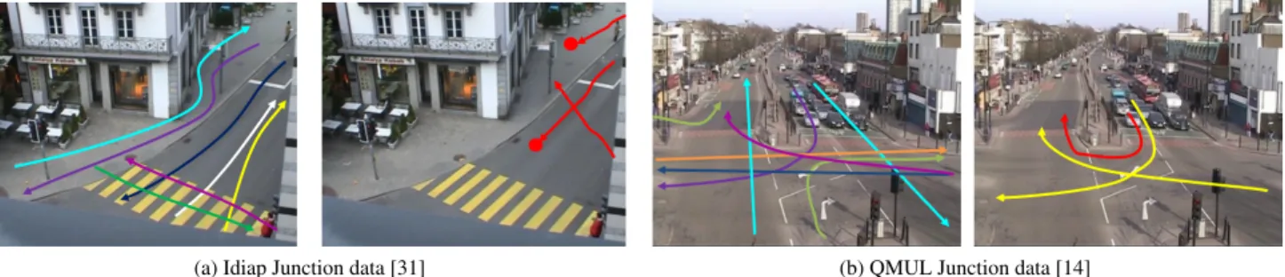
This work expressly focuses onabnormal event

detec-tionfrom surveillance feeds of traffic scenes (Fig.2). An-alyzing traffic scenes is challenging as a variety of events occur simultaneously, with vehicles moving in different di-rections at varying speeds along with pedestrians moving on sidewalks or crossing the road. Events of interest in such scenes include accidents, traffic congestion, abrupt changes in traffic patterns, pedestrian movement in prohibited areas and jay-walking. Automated detection of abnormal traffic events is formidable as they are often subtle and highly con-textual, and therefore difficult to model. Moreover, factors such as low video resolution, camera perspective, lighting changes, occlusions, variance in object size and motion and the rarity of anomalous exemplars strongly impede detec-tion.

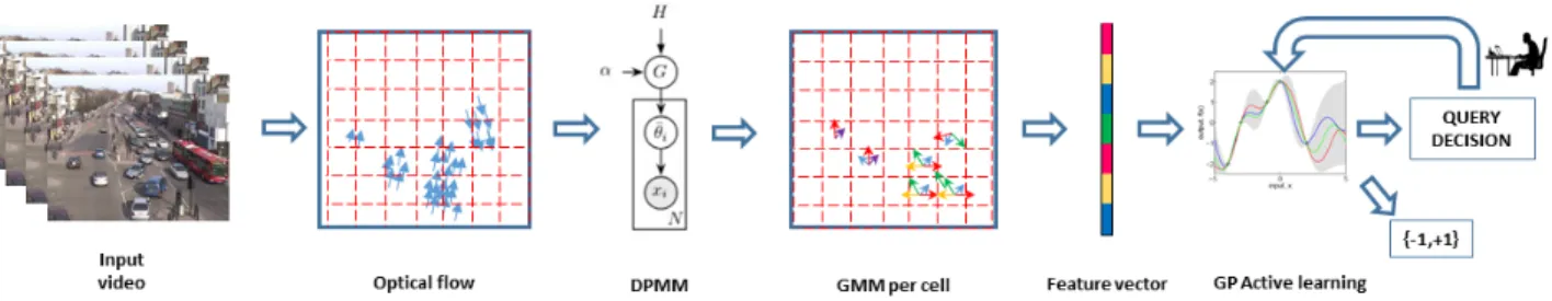
Prior traffic anomaly detection (AD) approaches [3, 31, 35] typically adopt an unsupervised, one-class learning ap-proach, where a model of normal behaviors is learned first, and used to subsequently detect abnormalities during the test phase. However, these methods do not effectively deal with the AD problem because of two main reasons: i) lack of effective video representations, and ii) the model of nor-mal behaviors is learned offline andnot updatedas new data arrive. To address this issue, we propose a non-parametric approach to anomaly detection that models local features more effectively and explores ahuman-in-the-loopAD sys-tem relying onactiveandonlinelearning framework, where a domain expert labels confusing (or alternatively, infor-mative) examples, which are then employed for refining the AD model (Fig. 1).

This work makes two research contributions. As our first contribution, we propose aDirichlet process mixture model (DPMM)-based modeling of object motion and di-rections within each cell of pixels to generate a fine-grained representation of scene activities. In contrast, traditional methods achieve unsupervised learning of coarse-grained scene activities which are often inadequate for AD. Also, since it would be unreasonable and expensive to query the

(a) Idiap Junction data [31] (b) QMUL Junction data [14]

Figure 2:Problem Illustration:One exemplar image from two traffic datasets is shown above. Arrows indicate direction of normal/abnormal activities. For each dataset, the left image shows normal activities, while the right image shows some ab-normal activity patterns (red arrows). Typical abab-normal activities include jay-walking by pedestrians, cars entering pedestrian zone (solid red dot), vehicles taking an illegal U-turn, near collisionsetc.(see Table 1).

Figure 1: Online and active anomalous event detection overview:Each video clip, represented in a feature space, is first put through a query criteria todecide whetherit is to be presented to the expert for labeling. Clips thus selected (as denoted by the orange dot) are actively labeled, and added to the existing list of labeled samples (events) for updating the classifier model.

expert for every clip (sample), confusing samples are de-termined such that AD performance improves after every query. To this end, our second contribution involves the proposition of a novel criterion, termedQrel, to evaluate if

a sample is to be queried for labeling. Qrel incorporates

and evaluates two related criteria, namely, (i)exploration– where sample labeling enables discovering unseen regions in the feature space, and (ii)exploitation, where sample la-beling refines inter-class boundaries as (orange sample in Fig.1). Furthermore, unlike AD methods (such as [5, 11]) that rely on batch-based active learning (AL), we propose an AL paradigm where samples aresequentiallyprocessed by the expert as in a real-life scenario. Different from previ-ous works [17, 18] which rely on simple classifiers, our AL module employs a more powerful Gaussian Process (GP)

classifier, and several interesting properties of GP motivated its choice for active AD: (i) Uncertainty measures such as

predictive meanandcovarianceof GPs naturally facilitate an AL paradigm [4, 11, 12]; (ii) Bayesian formulation of a GP allows for a sequential update of the AD model in closed-form [4], and (iii) The feature distributions of nor-mal activities varies smoothly over time, which is encapsu-lated by the GP covariance. Employing a GP classifier with ourQrel criterion enables superior performance relative to

other AL methodologies, as confirmed by experiments on two traffic surveillance datasets (illustrated in Fig. 2).

2. Related Work

Research areas closely related to this work are i) video representation for AD and ii) stream-based active learning. Below, we present a review of each of these topics.

Most existing work on abnormality detection rely on un-supervised methods to derive a representation of scene ac-tivities due to difficulty in labeling several hours of video data. Conventional AD methods are mostly trajectory based [19, 21, 25]. Here, object trajectories are used to learn dominant motion patterns of normal activities, which are then used for identifying outlier trajectories using likelihood measures [13,31] or classifiers such as one-class SVM [21]. Due to difficulties in obtaining reliable object trajectories, recent trends have explored variants of probabilistic topics models [15,31] and dynamic Bayesian networks [3,7,30] to describe a video clip via a learned patterns of activities. The activity patterns are in turn learned by applying topic mod-els such as probabilistic latent semantic analysis (pLSA) on low-level visual features from foreground pixels and their optical flow.

All aforementioned methods quantize (only) motion an-gles computed from optical flow vectors by determining the range of the quantization binsa-priori. While this approach is simple to use, it i) completely ignores object speed infor-mation that is readily available, ii) is not well adapted to the scene, and iii) results in large vocabularies when additional contextual cues are added. Furthermore, when scene

activ-ities are represented by mid-level topics learned from the scene, anomaly measures become less sensitive to changes or violations in low-level features.

To address these issues, we propose to quantize the flow vectors arising from each non-overlapping block of pixels1

using a Dirichlet process mixture model (DPMM), a non-parametric approach to learn mixture models that also infers the number of clusters in a data-driven manner. Learning a DPMM from optical flows results in a scene-centric vo-cabulary, while also incorporating both direction and speed information without increasing its size. Non-parametric methods, especially Hierarchical Dirichlet Processes [28] have been used by many earlier works [2, 17, 34] to model scene activities. Nevertheless, they are geared towards high-level learning of patterns and use pre-defined vocabularies. Another important problem faced by existing AD meth-ods is that they train a model in batch mode, which pre-cludes the interactive labeling of samples making them un-suitable for streamed data as typically encountered in real-life scenarios. In such cases,active learning (AL)would be an apt approach, where the aim is to improve a classi-fier incrementally by seeking labels on confused examples. AL paradigm has been used in computer vision to address problems including object classification [11], scene classi-fication [4, 12] and domain adaptation [16], where the fo-cus is mainly on designing efficient querying strategies that strike a trade-off betweenexplorationandexploitation. For instance, methods in [10, 29] predictive uncertainities for instance labeling and thus can be called exploitative as they aim to refine boundaries of known classes. On the other hand, explorative methods [20, 26] look for unknown re-gions in the feature space. This idea has been also employed to detect anomalies [20], traffic intrusions [26] and discover rare classes [5, 8]. Furthermore, several hybrid approaches including the unified theory in [9] combine both exploration and exploitation measures [4, 18] so that classification of known classes improves simultaneously with the discovery of new classes. For a more detailed review of AL methods, we refer to [24, 33]

Research works applying AL for surveillance have been very limited, as most well-known AL methods work on pool or batch-based settings, where samples are selected from a large pool of unlabeled samples for annotation by the domain expert, which only account for offline learning paradigms. In batch-based learning, a query criteria that gives a relative measure with respect to rest of the samples (e.g., ranked distance from the classification margin) is suf-ficient.

Surveillance settings are inherently stream based. There-fore, our goal is to decideon-the-fly whether or not to re-quest a label for an incoming sample. This requires more 1_{Each non-overlapping block of pixels also called cells is our basic unit}

for clip representation.

informative measures than distance ranks to be formulated. Our work is closely related to the work by [18], where a stream-based AL framework is developed via simple naive Bayes classifier which assumes that the individual features (activities in different scene regions) are independent given the class label. However, this assumption simplifies the fact that traffic scenes involvecomplex interactionsamong ac-tivities in different regions, and that scene acac-tivities are in-herently correlated. In contrast, we make use of predictive mean and covariance functions, as well as confidence in-tervals offered within the Bayesian formulation of GPs to formulate principled query strategies resulting in improved detection performance as shown in Section 5. The follow-ing section describes our proposed AD framework.

3. Problem Formulation

Consider a video stream composed of clips2_υ

tindexed by timet ∈ {1, . . . ,∞}. Each clip represented (in terms of events) asxt ∈ X,X ⊂IRDlying in aD dimensional space, belongs to one of two classes yt ∈ {−1,1}, with labels−1 and1denotingnormalandabnormalevents re-spectively. We seek to learn a classifierCthat best predicts a label yt for each clipxt. In order to acquire labels for classifier training and updation, we request a domain expert to label incoming samples (clips) for abnormal events (see Fig.1). Given a new sample, the decision to query the ex-pert for a label is taken based on a query functionQand a budgetB. The goal of functionQis to selectinformative samples that will help explore unseen regions in the feature space, while also refining decision boundaries to improve AD performance. Bis the limit on the number of queries made to buildC.

Fig. 3 presents the overall flowchart for our approach. The first step in our approach is to learn a DPMM model for each cell (10×10) of pixels. This model is learned from a training set comprisingnormalactivities. A feature vector that consolidates the activations from local DPMM models is used to describe each video clip, which is input to our GP-based active learning framework. Here, we first briefly review the basic concepts involved in our non-parametric modeling, i.e., i) Dirichlet process mixture model and ii) Gaussian Processes, followed by more precise details re-garding clip representation and Gaussian process learning.

3.1. Dirichlet Process Mixture Model

Dirichlet process mixture models (DPMM) can be con-sidered as an infinite extension of the finite mixture model. Therefore, it may be easy to understand a DPMM starting from a finite mixture model. Fig. 4(a) is a graphical rep-resentation of a finite mixture model withK components. Theβ vector gives the weight of each mixture component 2_{snippets capturing concurrent events some of which may be abnormal.}

Figure 3: Flowchart of our non-parametric active online AD framework. Optical flow vectors observed from each cell of 10×10pixels over normal clips are used to learn a DPMM model for each cell. Every video clip is then represented by a feature vector obtained by concatenating the activations in each cell’s DPMM, which is fed into the Gaussian process-based active learning framework. A decision is made instantaneously whether or not to query an expert for a label corresponding to the sample. a) zi N(obs. i) xi α K Φk H β b) zi N(obs. i) θi α c) θi N(obs. i) xi α G H

Figure 4: Finite mixture and Dirichlet Process (infinite mix-ture): a) finite mixture withKelements; b) mixture repre-sentation for DP; c) compact reprerepre-sentation for DP.

andαis a prior on these weights. EachΦk represents the parameters of a mixture component andzirepresents the in-dex of the mixture component for each observationxi. The mixture components we are using here are Gaussian distri-butions (Φk = (µk,Σk)), finally resulting in a Gaussian mixture model (GMM).

β ∼GEM(α) (1)

∀k φk ∼H (2)

∀i zi∼Categorical(β) (3)

xi∼φzi =N(xi|µzi,Σzi) (4)

By letting K go to infinity, we obtain an infinite mixture model as shown in Fig. 4(b). We can explicitly represent the mixture component selected by each observation noted

θi. We use dashed arrows to indicate deterministic relations, hereθi = Φzi(or, expressed as a draw from a Dirac

distri-bution: θi ∼ δΦ_zi). To adapt to this infinite mixture

ele-ments, the weight vectorβis of infinite length and the prior

αtakes a specific form. Theαprior is now a single positive real value used as the parameter of a “GEM” (Griffiths, En-gen, McCloskey) also known as a “stick breaking” process. This process produces an infinite list of weights that sum to 1: the first weightβ1=β10 is drawn from a beta distribution

Beta(1, α), the second weight is drawn in the same way but

only from the remaining part,i.e.,β2= (1−β1)∗β02with

β₂0 drawn fromBeta(1, α), and so on for the other weights, hence the “stick breaking” name. For each mixture com-ponent, the parametersΦk are independently drawn from a priorH. We thus have the following:

A more compact equivalent notation can be used to rep-resent a Dirichlet Process. While the mixture reprep-resentation is well adapted for deriving the Gibbs sampling scheme, a more compact representation as shown in Figure 4c is widely used to represent a DPMM. Here, individual mix-ture components are not shown and instead their weighted countable infinite mixtureG =P∞

k=1βkδφk is used. The

corresponding representation, using a DP notation, is given as:

G∼DP(α, H) (5)

∀i θi∼G (6)

xi∼θi (7)

We need to specify the base distributionH to complete the model. We use a Normal- Inverse Wishart distribution for the base distributionH as it acts as a conjugate for Normal distribution and simplifies the inference process. The hyper parameters for the base distribution areµ0, λ0,Σ0, ν0 and

the concentration parameterα, which controls the number of Gaussian components. The DPMM is solved by esti-mating the posterior distribution using Gibbs sampling. We refer to [27] for more details on this.

3.2. Gaussian Process

Given a dataset D = {(xi, yi)}Ni=1 comprising N

feature-label pairs where xi andyi are defined as above, our objective is to predict the label y∗ of an unseen

sam-ple x∗. We assume that the relationship between xi and labels yi is given by a latent function f : X → IR and additive Gaussian noise leading toyi = f(xi) +, where

∼N(0, σ2

parametric family of functions, we assume thatf is drawn from a specific probability distributionp(f). This enables a Bayesian treatment of our problem,i.e., we infer the prob-ability ofy∗givenx∗ and old observationsDby

integrat-ing out the correspondintegrat-ing function valuesf∗ =f(x∗)and f ={f1, . . . , fN}: p(y∗|x∗,D, θ) = Z p(f∗|x∗,D, θ)p(y∗|f∗)df∗, (8) p(f∗|x∗,D, θ) = Z p(f∗|x∗,f, θ)p(f|D, θ)df, (9)

whereθ denotes model hyper-parameters. In GP, we as-sume that the prior distribution over function values is given by a multivariate Gaussian distribution, denoted asp(f) =

N(m(X), κ(X, X)), wherem(.)is the mean function and

κ(., .)is the covariance function (anN ×N matrix whose (i, j)th _{element is given by a kernel function κ(x}

i,xj)), which describes the coupling betweenxiandxjas a tion of their distance. A popular choice for the kernel func-tion is the squared exponential given by,

κ(xi,xj) =σn2exp(− D X k=1 (xik−xjk)2 2σ2 k ), (10) whereσ2

nrepresents signal noise andσkdenotes scaling pa-rameter for dimensionk. The posterior predictive distribu-tion given in Eq.(9) is again Gaussian with moments:

µ∗(x∗) =k∗T(K+σ2nI) −1_{Y (11)} σ_∗2(x∗) =k∗∗+σ2n−k T ∗(K+σ2nI) −1_k ∗, (12)

whereY = [y1, . . . , yN]T,K,k∗ andk∗∗ respectively

de-note the N ×N kernel matrix containing covariances of training samples, the(N ×1)kernel vector containing co-variances between training samples and the test sample, and the covariance of the test sample to itself.

We can deduce from Eq.(10) thatκ(xi,xj)approaches its maximum valueσ2

nwhenxi ≈xjdenoting thatfiand

fj are nearly perfectly correlated, whereask(xi,xj) ≈ 0 when xi is far from xj indicating minimum influence xi has on xj. For binary classification problem, probability of y is independent of all other quantities given the value of f(x), i.e.,p(y = 1|D, f(x)) = p(y = 1|f(x)). The likelihood functionp(y|f(x))is usually modeled using cu-mulative normal (CN). This function maps high values off

to≈1and lowfto≈0.

Note that due to the Gaussian noise assumption that links

y∗ andf∗, their expected values are the same. However, their variances differ owing to observational noise. Due to this fact, a test sample x∗ can be classified based on the

sign ofµ∗(x∗), and the absolute predictive mean|µ∗(x∗)|

indicates how close or far the sample is to the classification boundary. A small absolute mean indicates that the sample lies close to the boundary and hence is a confusing case

and vice-versa. Labeling samples near the class boundary is critical, as these may indicate abnormal events that may be potentially confused with normal events or false negatives. Also, labeling such samples can refine the class boundary leading to anexploitativestrategy. In contrast to the pool-based setting, where a sample for querying is chosen by ranking absolute predictive mean values obtained for a pool of unlabeled data, we need to derive an absolute criterion to decide on-the-fly if a sample needs querying or not. We formulate this by placing a threshold on|µ∗(x∗)|,i.e., we

decide to query for a sample label if|µ∗(x∗)|is close to

zero or, Qµ : |µ∗(x∗)| ≤ τ1, whereτ1 is a threshold. In

particular, we are interested in points for which CN is≈0.5, which happens when|µ∗(x∗)| ≈0.

Another criterion is to query for samples with large pre-dictive variance Qvar(x∗) = σ∗2(x∗). A largeσ2∗(x∗)

in-dicates that the sample lies in an unexplored region of the feature space, potentially denoting outlier clips. Labeling such samples help us explore unknown abnormality types leading to anexplorativestrategy. An uncertainty measure which considers both the predictive mean and variance is proposed in [11]. Specifically, the query criterion is given by:Qunc(x∗) =√|µ∗(x∗)|

σ2

∗(x∗)+σn2

This criterion combines both exploration and exploitation. However, this method focuses more onoutliersamples that are far from training samples than confusing ones [10]. As abnormal events typically oc-cur with other normal events and have limited spatial and temporal support, they lie close to normal events and de-note confusing samples rather than outliers.

We formulate a new and more severe criterion that com-bines both exploration and exploitation, and ranks both pre-dictive mean and variance for label querying: Qrel(x∗) =

min{2|µ∗(x∗)|,_σ∗(2_x∗)}. A label is sought for samples

when Qrel(x∗) < τ2, where τ2 denotes a user-defined

threshold. Here, the idea is to choose samples for which at least one of the (mean or variance) criteria indicate that the sample needs to be queried. When τ2 = 1, samples

are either very close to the class boundary or have a pre-dictive standard deviation greater than 2, indicating they are far from (>95%) of training samples. SinceQrel decides

to query for labels on checking whether the mean or vari-ance is relatively more important, it is a Relative Impor-tancecriterion. Empirical results confirm the suitability of this criterion for active AD.

4. Video representation

Since videos need to be characterized in terms of activi-ties for our problem, we derive a clip representation derived from low-level motion cues. Upon splitting a video into short clips, we track moving objects via densely sampled feature points [32], with the maximum trajectory length set to 15 frames. Location and motion information available

Table 1: Abnormal events from the two considered datasets.

Description # clips (%)

Idiap

Car stopping abruptly after traffic light 21 (1.58) Pedestrians Jaywalking 146 (11.0) Car entering pedestrian area 47 (3.5) QMUL

Illegal U-turn 29 (1.61) Emergency vehicles using incorrect lane 3 (0.17)

Traffic halt due to fire engine 12 (0.67) from trajectory observations are quantized to a feature vec-tor representation for each clip. Quantization steps for vo-cabulary creation are:

Activities in surveillance videos captured by fixed cam-eras can be characterized by their location. We quantize pixel positions into non-overlapping cells of10×10pixels.

E.g.,we obtain29×36cells from a288×360pixel video. From consecutive trajectory observations, we compute mo-tion vectors(ux, uy). The inputs to our DPMM model for each cell are motion vectors observed in the cell from a set of normal clips. The DPMM components are then learned using the Chinese restaurant process and Gibbs sampling as detailed in [27]. Additionally, in order to capture unfore-seen motion within each cell (which possibly might indicate anomolies), we add a background Gaussian component with parameters (µbg= 0,Σbg= 4, βbg= 0.1) to every cell. For cells with a DPMM model, this component is simply added to the existing mixture components followed by a renormal-ization of the prior weight parameter.

Each cell c is then represented using a weight vector wc of lengthdc + 1, wheredc is the number of Gaussian components discovered for each cellc. The weight vector wc is obtained by summing the posterior probability vec-tors from every single observation in that cell. The video clip is finally represented by stacking all the weight vec-tors(w1,· · ·,wNc)followed by a normalization so that the

sum of all weights is one. HereNcis the number of cells in the image.

5. Experimental Results

Datasets: We report experiments on two public video datasets specified in Table 1. TheIdiap Junction data[31] (Fig.2(a)), is a video from a busy road junction. The video is 44 minutes long, and recorded at 25 fps with a frame size of360×288. Activities at the junction include (a) people walking on the pavement, (b) people waiting for vehicles to cross, (c) people crossing at zebra crossings, (d) vehi-cles moving in different directionsetc.TheQMUL Junc-tion data[14] (Fig.2(b)) is filmed at a four-road junction. The video is 1 hour (90000 frames) long, recorded at 25 fps at360×288resolution. The junction is regulated by traf-fic lights and dominated by four types of traftraf-fic flows. Ta-ble 1 describes the abnormal activities in these two datasets. The number of clips involving abnormal activities, and the proportion of such clips over the video length (in %) are

specified in the right column. Both videos were segmented into short clips of 50 frames. This results in 1327 and 1800 clips for the Idiap and QMUL data respectively. For Idiap, events in each clip were manually annotated as nor-mal/abnormal, while annotations were obtained from [18] for QMUL. Ground-truth labels were used for simulating theexpert labelduring queries, and for performance evalu-ation.

Settings:The DPMM model is first learned using 450 nor-mal clips corresponding to 15 minutes of video. We use a Normal-inverse Wishart for the based distribution of the model with the parameters set asµ0= (0,0), λ0= 4,Σ0=

I, ν0 = 2. The concentration parameter of DPMM, which

controls the number of clusters, is set to a default value of

α = 0.1. The number of mixture components learned for each cell varies between 2-12 in the Idiap junction dataset and 2-8 in the QMUL junction dataset. The relatively higher number of components for the Idiap dataset may be due to the large number of pedestrian motion observed in the scene, which is more unstructured compared to vehicles. This results in a total of 3882 and 3218 components for the Idiap and QMUL Junction dataset, which has fewer dimen-sions compared to a predefined quantization3_.

Clips from each video were partitioned into training and test sets– 60% clips were used for training and the remain-ing for test. To begin with, a simple GP classifier was learned using two clips containing normal activities and one clip involving unusual event(s). The remaining training samples were visited sequentially, and were either queried for a label or discarded. Upon adding a newly (actively) labeled sample to the training set, the classifier was up-dated and its performance evaluated on the test set. For each dataset, we created 10 different sequences by ran-domly shuffling the training clips. Performance was mea-sured by computing the area under the receiver operator curve (AUROC) after each query. Final curves (Fig.6) were obtained on averaging the AUROC values over the 10 runs. Kernel computation is a key component of GP classification. Histogram intersection kernel (HIK), given by KHI(Z,Z0) = P

NA

i=1min{zi, z0i}, which generates a positive-definite matrix was efficiently used for covariance computation for GP [23]. Since the feature vector repre-senting each clip is a topic weight vector or normalized his-togram, we used HIK for covariance computation. We used the GPML library [22] for active learning and implemented the DPMM model from scratch in Matlab.

Baselines: We perform experiments to evaluate i) our clip representation method and ii) our query criteria. First, to perform comparative evaluation of our clip representation method, we consider two other baseline approaches. a) 3_{From a frame size of360×288pixels, we get 4176 words by}

Figure 5:DPMM result from TJ and QMUL datasets:For each cell, the top ranking Gaussian component is demonstrated using arrows emerging from the location. For convenience, they are separated into different directions and color coded. a) column 1 - Red (270◦−45◦), column 2 - egreen (270◦−225◦), column 3 - blue (225◦−135◦) and column 4 - magenta (135◦−45◦). Length of the arrows are scaled based on their magnitude indicating speed.

(a) (b) (c) (d)

Figure 6: Comparison of clip representation methods and AL query criteria:(a,b) results from different clip represen-tation methods using the proposed Rel-Importance query strategy on (a) QMUL and (b) Idiap junction data. Results from different AL query strategies within the Gaussian Process framework for (c) QMUL and (d) Idiap junction data (best viewed in color and under zoom).

we implemented a predefined coarse vocabulary creation method followed in several earlier works [31, 34] Here, lo-cation is quantized into 10x10 cells and motion direction is quantized into four labels (left, right,up, down) corre-sponding to the cardinal motion directions. Each video clip (ordocument)υis represented by the frequencyn(υ, w), of a wordwoccurring inυto obtain the bag-of-words repre-sentation. We denote this by the namePredefined. b) For the second baseline, we apply a dimensionality reduction method using Latent Dirichlet Allocation (LDA) [1] learned on a few normal activity clips to discoverNAdominant top-ics indicated byZ={z1, . . . , zNA}. Subsequently, the

fea-ture vectorxfor everyυis given by the topic weight vector (p(z1|υ), . . . , p(zNA|υ))obtained by the folding-in

proce-dure [6], where each entry indicates the extent of topic zi

present in υ. We used 30 topics to represent each clip in our experiments. We denote this by the nameLDA topics

in our evaluation.

We compare the AUROC obtained usingQrelwith

var-ious other query criteria. They include predictive mean (pred-mean/ Qµ), predictive variance (pred-var/Qvar) and

the uncertainty criteria (unc/Qunc) proposed by [11, 23].

Thresholds to select samples forQµ,Qvar andQuncwere

fixed as 1, 2 and 0.5 respectively. We also use a ran-dom/Qrandcriteron, where samples are queried or rejected

with equal probability. Furthermore, we also learned a one-class SVM (referred as 1-SVM in Fig.6) using only normal documents that are used by the aforementioned active learn-ing methods.

directions corresponding to each cell obtained by applying DPMM on the two datasets. Note that the length of the ar-rows are weighted by the magnitude of the mean motion vector. Interestingly, we see motion vectors with higher speed from cells close to the camera (cf. last column in Fig. 5) due to perspective effect of the camera.

In Fig. 6(a,b) we evaluate the performance of our active learning method using different clip representation meth-ods, by fixing the query criteria toQrel. Thanks to the

ef-fective modeling of local activities by DPMM, we observe a much higher AUR by the proposed method compared to the other two baselines. Interestingly, the performance due to the predefined vocabulary and LDA topics are quite similar. This can be due to the fact that LDA topics are learned from the same predefined vocabulary.

Fig. 6(c,d) compares AUROCs obtained from classifica-tion accuracies evaluated on the abnormal clips with dif-ferent query strategies on the two datasets, where our pro-posed DPMM based clip representation is used. Firstly, we observe that the classifier performance improves as queries are progressively made, however saturating after about 80 queries indicating that further labeled samples do not im-prove AD performance. Best performance is obtained us-ing ourQrelcriterion, resulting in a peak AUC performance

of 87% for QMUL, and 76% AUC for Idiap. Qµ is the next best performing criterion, thereby revealing that query criteria focusing on refining class boundaries and resolv-ing confusions perform best for the AD problem. This is in line with our understanding that most of the abnormal clips remain close to the normal clips in the feature space and hence contribute to confusions between the classes. We also see that Qvar and Qunc [11] perform similarly, but

with lower accuracy thanQrelandQµ. This is mainly

be-cause normal and abnormal events are closely clustered in the feature space, and hence looking for outliers as inQvar

does not yield the best results. Expectedly, the batch mode 1-SVM performs just better than random with about 57% and 56% accuracy on the QMUL and Idiap datasets respec-tively. The random query criteriaQrandstill improves over

1-SVM, but performs worse than others. Finally, a compre-hensive comparison combining different clip representation methods with different query criteria is presented in Fig. 7. Again, we see that the combination of DPMM andQrel cri-teria gives the best results in both the cases.

Discussion: In order to better understand the effect of the threshold on Qrel to select a query instance, we experi-mented with a range of threshold values from the interval [0.1,2]. From our results, we found that our method is not too sensitive to this threshold and the performance remains unchanged until reduced below 0.5 or increased above 1.5. In the former case (<0.5), a conservative threshold missed several interesting samples for label query leading to small performance improvements. In the latter case (> 1.5),

Figure 7:Comprehensive comparison.comparative study of various combinations ofQand clip representation meth-ods (left) QMUL [14] and (right) Idiap [31] junction data (best viewed in color). The results shown are obtained after running AL with a budgetB= 60%of training data. several uninformative samples are selected for label query. This exhausts the budget quickly with only little improve-ment. In our case, setting this to 1 was a good compromise. Since our approach combines two different measures, it is also interesting to understand which measure triggers most of the queries. Our analysis revealed that the predicitive mean (first factor in Qrel) triggered nearly85% and82% of the queries in the QMUL and Idiap junction datasets re-spectively, with the remaining queries triggered by higher predicitive variance. This concurs with our observation that anomalies are subtle and often co-occur with other normal activities, leading to clips that are confusing (determined by uncertainty criteria) rather than being an outlier. This is also reflected in the performance curves presented in Fig. 6(c,d), where we see that predictive mean is the second best per-forming query criteria and often close to the proposed ap-proach.

6. Conclusion

This paper proposes an active and online anomaly detec-tion system. Different from prior active learning methods proposed for surveillance scenarios which employ batch-based model training, our methodology accounts for real-life situations where video snippets are processed sequen-tially, followed by evaluation via the query criterionQrelto

decide if an event needs to be labeled by the domain expert. The criterionQrelused to identifyinformativesamples,

in-corporates the twin criteria of exploration and exploitation. Furthermore, a fine-grained representation of scene activi-ties is extracted via a Dirichlet process mixture model that enables better context modeling in terms of speed and mo-tion direcmo-tion. Experiments on two traffic datasets show that

Qrel outperforms competing query criteria for active

learn-ing.

Acknowledgments:This work is supported by the research grant for the Human-Centered Cyber-physical Systems Pro-gramme at the Advanced Digital Sciences Center from Sin-gapore’s Agency for Science, Technology and Research (A*STAR). We thank NVIDIA for GPU donation.

References

[1] D. M. Blei, A. Y. Ng, and M. I. Jordan. Latent dirichlet allo-cation. Journal of Machine Learning Research, 3(4-5):993– 1022, 2003.

[2] R. Emonet, J. Varadarajan, and J.-M. Odobez. Extracting and locating temporal motifs in video scenes using a hierar-chical non parametric bayesian model. InIEEE Conference on Computer Vision and Pattern Recognition, 2011. [3] R. Emonet, J. Varadarajan, and J.-M. Odobez. Multi-camera

open space human activity discovery for anomaly detec-tion. InIEEE Conference on Audio and Video Signal based Surveillance, 2011.

[4] A. Freytag, E. Rodner, P. Bodesheim, and J. Denzler. La-beling examples that matter: Relevance-based active learn-ing with gaussian processes. InGerman Conference Pattern Recognition, 2013.

[5] T. S. F. Haines and T. Xiang. Active rare class discovery and classification using dirichlet processes. International Jour-nal of Computer Vision, 106(3):315–331, 2013.

[6] T. Hofmann. Unsupervised learning by probability latent semantic analysis. Journal of Machine Learning Research, 42:177–196, 2001.

[7] T. Hospedales, S. Gong, and T. Xiang. A Markov clustering topic model for mining behavior in video. InIEEE Interna-tional Conference on Computer Vision, Kyoto, Japan, 2009. [8] T. M. Hospedales, S. Gong, and T. Xiang. Finding rare

classes: Adapting generative and discriminative models in active learning. InAdvances in Knowledge Discovery and Data Mining: 15th Pacific-Asia Conference, 2011.

[9] T. M. Hospedales, S. Gong, and T. Xiang. A unifying theory of active discovery and learning. InEuropean Conference on Computer Vision, 2012.

[10] P. Jain and A. Kapoor. Active learning for large multi-class problems. InCVPR, 2009.

[11] A. Kapoor, K. Grauman, R. Urtasun, and T. Darrell. Active learning with gaussian processes for object categorization. In

CVPR, 2007.

[12] M. Kemmler, E. Rodner, E.-S. Wacker, and J. Denzler. One-class One-classification with gaussian processes. Pattern Recog-nition, 46(12):3507 – 3518, 2013.

[13] J. Kim and K. Grauman. Observe locally, infer globally: a space-time mrf for detecting abnormal activities with incre-mental updates. InCVPR, 2009.

[14] J. Li, S. Gong, and T. Xiang. Global behaviour inference us-ing probabilistic latent semantic analysis. InBritish Machine Vision Conference, 2008.

[15] J. Li, S. Gong, and T. Xiang. Discovering multi-camera be-haviour correlations for on-the-fly global activity prediction and anomaly detection. InIEEE International Workshop on Visual Surveillance, Kyoto, Japan, 2009.

[16] G. Liu, Y. Yan, R. Subramanian, J. Song, G. Lu, and N. Sebe. Active domain adaptation with noisy labels for multimedia analysis.World Wide Web, 19(2):199–215, 2016.

[17] C. C. Loy, T. M. Hospedales, T. Xiang, and S. Gong. Stream-based joint exploration-exploitation active learning. InCVPR, 2012.

[18] C. C. Loy, T. Xiang, and S. Gong. Stream-based active un-usual detection. InACCV, 2012.

[19] V. Mirge, K. Verma, and S. Gupta. Dense traffic flow pat-terns mining in bi-directional road networks using density based trajectory clustering. Advances in Data Analysis and Classification, pages 1–15, 2016.

[20] D. Pelleg and A. Moore. Active learning for anomaly and rare-category detection. In NIPS, pages 1073–1080. MIT Press, 2004.

[21] C. Piciarelli, C. Micheloni, and G. L. Foresti. Trajectory-based anomalous event detection.IEEE Trans. Cir. and Sys. for Video Technol., 18(11):1544–1554, Nov. 2008.

[22] C. E. Rasmussen and H. Nickisch. Gaussian processes for machine learning (gpml) toolbox. J. Mach. Learn. Res., 11:3011–3015, 2010.

[23] E. Rodner, A. Freytag, P. Bodesheim, and J. Denzler. Large-scale gaussian process classification with flexible adaptive histogram kernels. InECCV, 2012.

[24] B. Settles. Active learning literature survey. Technical report, University of Wisconson-Madison, 2010.

[25] R. Sharma and T. Guha. A trajectory clustering approach to crowd flow segmentation in videos. InIEEE International Conference on Image Processing (ICIP), pages 1200–1204, 2016.

[26] J. W. Stokes, J. C. Platt, J. Kravis, and M. Shilman. Aladin: Active learning of anomalies to detect intrusions, microsoft research. Technical report, MSR, 2008.

[27] E. Sudderth.Graphical models for visual object recognition and tracking. PhD thesis, MIT, 2006.

[28] Y. W. Teh, M. I. Jordan, M. J. Beal, and D. M. Blei. Hierar-chical Dirichlet processes. Journal of the American Statisti-cal Association, 101(476):1566–1581, 2006.

[29] S. Tong and D. Koller. Support vector machine active learn-ing with applications to text classification. J. Mach. Learn. Res., 2:45–66, 2002.

[30] J. Varadarajan, R. Emonet, and J. Odobez. Bridging the Past, Present and Future; Modeling Scene Activities from Event Relationships and Global Rules. Providence, USA, 2012. [31] J. Varadarajan and J. Odobez. Topic models for scene

analy-sis and abnormality detection. InIEEE International Work-shop on Visual Surveillance, Kyoto, Japan, 2009.

[32] H. Wang, A. Kl¨aser, C. Schmid, and C.-L. Liu. Action Recognition by Dense Trajectories. InCVPR, 2011. [33] M. Wang and X.-S. Hua. Active learning in multimedia

an-notation and retrieval: A survey. ACM Trans. Intell. Syst. Technol., 2(2):10:1–10:21, Feb. 2011.

[34] X. Wang, X. Ma, and E. L. Grimson. Unsupervised activ-ity perception in crowded and complicated scenes using hi-erarchical bayesian models. IEEE Transactions on Pattern Analysis and Machine Intelligence, 31(3):539–555, 2009. [35] G. Zen and E. Ricci. Earth mover’s prototypes: A

con-vex learning approach for discovering activity patterns in dy-namic scenes. InCVPR, pages 3225–3232. IEEE, 2011.