Estimating the Health Effects of Environmental Exposures: Statistical Methods for the Analysis of Spatio-temporal Data

Estimating the Health Effects of Environmental Exposures:

Statistical Methods for the Analysis of Spatio-temporal Data

(Article begins on next page)

The Harvard community has made this article openly available.

Please share

how this access benefits you. Your story matters.

Citation

Correia, Andrew William. 2013. Estimating the Health Effects of

_{Environmental Exposures: Statistical Methods for the Analysis of}

Spatio-temporal Data. Doctoral dissertation, Harvard University.

Accessed

Citable Link

http://nrs.harvard.edu/urn-3:HUL.InstRepos:11158266

Terms of Use

This article was downloaded from Harvard University's DASH

_{repository, and is made available under the terms and conditions}

applicable to Other Posted Material, as set forth at

http://nrs.harvard.edu/urn-3:HUL.InstRepos:dash.current.terms-of-use#LAA

Estimating the Health Effects of Environmental

Exposures: Statistical Methods for the Analysis of

Spatio-temporal Data

A dissertation presented

by

Andrew William Correia

to

The Department of Biostatistics

in partial fulfillment of the requirements

for the degree of

Doctor of Philosophy

in the subject of

Biostatistics

Harvard University

Cambridge, Massachusetts

April 2013

©2013 - Andrew William Correia All rights reserved.

Advisor: Professor Francesca Dominici Andrew William Correia

Estimating the Health Effects of Environmental Exposures:

Statistical Methods for the Analysis of Spatio-temporal

Data

Abstract

In the field of environmental epidemiology, there is a great deal of care required in constructing models that accurately estimate the effects of environmental exposures on human health. This is because the nature of the data that is available to researchers to estimate these effects is almost always observational in nature, making it difficult to ade-quately control for all potential confounders - both measured and unmeasured. Here, we tackle three different problems in which the goal is to accurately estimate the effect of an environmental exposure on various health outcomes.

In Chapter 1, we extend and expand upon a previous study examining the relation-ship between fine particle air pollution and life expectancy in the United States (US) by analyzing data from the period 2000 to 2007 from 545 counties across the US. Using straightforward regression techniques, we estimate the association between changes in air pollution levels and changes in life expectancy over the period from 2000 to 2007 for the entire US as well as for a number of subpopulations within the US.

Chapter 2 builds upon the previous chapter by developing a modeling approach for estimating the effects of monthly variations in fine particle air pollution on monthly vari-ations in mortality while controlling for potential sources of confounding. We first show via a simulation study where previous approaches to estimating this relationship break down. We then propose a new model to overcome those deficiencies, and we evaluate this approach using a large Medicare dataset linked with air pollution exposure estimates

In Chapter 3, we evaluate the impact of noise exposure from airports on hospital-izations for cardiovascular disease (CVD) among Medicare enrollees living in zip codes surrounding major airports in the continental US. We begin with a fully Bayesian hierar-chical Poisson model for the expected number of CVD hospitalizations in each zip code as a function of exposure to noise as well as several other individual and area-level co-variates. We then conduct a thorough sensitivity analysis, examining potential sources of confounding, spatial dependence, and the possibility of a threshold effect.

Contents

1 The Effect of Air Pollution Control on Life Expectancy in the United States: An Analysis of 545 US counties for the period 2000 to 2007 1 1.1 Introduction . . . 2 1.2 Methods . . . 3 1.2.1 Data . . . 3 1.2.2 Statistical Analysis . . . 7 1.3 Results . . . 8 1.4 Discussion . . . 21

2 A Closer Look at Exposure Decomposition in Long-term Air Pollution Studies: A Distributed Lag Approach 26 2.1 Background . . . 27

2.2 Overview of Methodology and Modeling Assumptions . . . 28

2.3 Simulation Study . . . 30

2.3.1 Equality ofη1 andη2 . . . 30

2.3.2 Size of the Window for Averaging Monthly Air Pollution . . . 34

2.5 Methods . . . 42

2.5.1 Statistical Approach . . . 42

2.6 Results . . . 44

2.7 Discussion . . . 50

3 Exposure to Aircraft Noise and Hospital Admissions for Cardiovascular Dis-eases: A Large National Multi-Airport Population Cohort Study 54 3.1 Introduction . . . 55

3.2 Methods . . . 56

3.2.1 Noise Exposure Estimates . . . 56

3.2.2 Statistical Methods . . . 58

3.3 Results . . . 61

3.4 Sensitivity Analyses . . . 76

3.4.1 Residual Spatial Confounding . . . 76

3.4.2 Modeling Spatial Dependency . . . 80

3.4.3 Threshold Effects and Non-linearity in the Exposure Response Curve 84 3.5 Discussion . . . 85

Appendix 91

Acknowledgments

I would like to thank my advisor, Francesca Dominici, for being an excellent mentor, and for her support, positive energy, and commitment to not only me, but to everyone in our group.

I would also like to thank my committee members Jonathan Levy and Brent Coull for their guidance and feedback, as well as Arden Pope, Majid Ezzati, and Doug Dock-ery who all played a significant role in my development as a graduate student. I feel quite fortunate to have had a chance to work with each these very talented and dedicated people.

I am extremely grateful to my parents, Gil and Gabriela Correia, whose love and support helped me to become the person I am today. Thank you for always encouraging me, for always pushing me to do better, and for never letting me quit anything I started.

Lastly, I would like to thank my beautiful bride to be, Andrea Saunders. Thank you for always being there, no matter what.

The Effect of Air Pollution Control on Life Expectancy in

the United States: An Analysis of 545 US counties for the

period 2000 to 2007

Andrew W. Correia

, C. Arden Pope III

, Douglas W. Dockery

, Yun

Wang

, Majid Ezzati

, and Francesca Dominici

1

_{Department of Biostatistics, Harvard University}

_{Department of Economics, Brigham Young University}

_{Departments of Environmental Health and Epidemiology,}

Harvard School of Public Health

4

_{MRC-HPA Centre for Environment and Health and Department of}

1.1

Introduction

Since the 1970s, enactment of increasingly stringent air quality controls has led to improvements in ambient air quality in the United States at costs that the U.S. En-vironmental Protection Agency (EPA) has estimated as high as $25 billion per year {United States Environmental Protection Agency (1997)}. However, even with the well-established link between long-term exposure to air pollution and adverse effects on health {Pope (2007)}, the extent to which more recent regulatory actions have benefited public health remains in question.

Air pollutant concentrations have been generally decreasing in the U.S., with sub-stantial differences in reductions across metropolitan areas. Levels of fine particulate mat-ter air pollution (particulate matmat-ter< 2.5µg/m3 in aerodynamic diameter,PM2.5) remain

relatively high in some areas. In a 2010 study, the EPA estimated that 62 U.S. counties, ac-counting for26%of their total study population, hadPM2.5concentrations not in

compli-ance with the National Ambient Air Quality Standards (NAAQS) {Schmidt et al. (2010)}. Reductions in particulate matter air pollution are associated with reductions in both cardiopulmonary and overall mortality {Pope (2007)}. In the mid-1990s, the Har-vard Six Cities Study and the American Cancer Society (ACS) study reported associations of cardiopulmonary mortality risk with chronic exposure to fine particulate air pollution while controlling for smoking and other individual risk factors {Dockery et al. (1993); Pope et al. (1995)}. Reanalysis and extended analyses of these studies have confirmed that fine particulate air pollution is an important independent environmental risk factor for cardiopulmonary disease and mortality {Krewski et al. (2000); Pope et al. (2002, 2004); Jerrett et al. (2005); Laden et al. (2006); Krewski et al. (2005b,a)}. Additional cohort stud-ies, population-based studstud-ies, and short-term time-series studies have also shown asso-ciations between reductions in air pollution and reductions in human mortality {Burnett et al. (2001); Samet et al. (2000); Schwartz et al. (2008); Evans et al. (1984); Özkaynak and Thurston (1987); Pope and Dockery (2006); Schwartz (1991, 1992); Dominici et al. (2003)}.

More recently, studies have suggested an association betweenPM2.5 and life expectancy

{Tainio et al. (2007); Pope et al. (2009)}, a well-documented and important measure of overall public health {Brunekreef (1997); McMichael et al. (1998); Rabl (2003)}.

As our primary analysis, we estimate the association between changes inPM2.5and

in life expectancy in 545 U.S. counties during the period 2000 to 2007. This period is of particular interest, as the EPA restarted wide collection ofPM2.5 data in 1999 - 2000, after

stopping the nationwide PM2.5 monitoring program during the mid-1980s and most of

the 1990s. In secondary analyses, we extended the data and statistical analysis originally reported by Pope et al. (2009) for the period 1980 - 2000 to 2007, and investigated whether the relationship reported by Pope et al. (2009) persists in the more recent years.

1.2

Methods

1.2.1

Data

We constructed and analyzed three data sets to estimate the association between changes in life expectancy and changes in PM2.5 during the period 2000 to 2007 in 545

counties (Dataset 1), and to investigate whether the association previously reported by Pope et al. (2009) persists when the data on the same 211 counties are extended to the year 2007 (Datasets 2 and 3).

Dataset 1 included information on 545 U.S. counties for the years 2000 and 2007. These counties include all counties with available matchingPM2.5data for 2000 and 2007.

Additionally, unlike previous work in which counties were located only in metropoli-tan areas Pope et al. (2009), Dataset 1 is comprised of counties in both metropolimetropoli-tan and non-metropolitan areas. Figure 1.1 shows the counties in this dataset shaded ac-cording to life expectancy in 2000 and 2007. Variables in this dataset were available at the county level, for both 2000 and 2007, and included: life expectancy, PM2.5, per

propor-tions who were white, black, or Hispanic. Because data on smoking prevalence were not available for all 545 counties, we used age-standardized death rates for lung can-cer and chronic obstructive pulmonary disease (COPD) as proxy variables for smoking prevalence {Peto et al. (1992); Eftim et al. (2008)}. Death rates were calculated in 5-year age groups and age-standardized for the 2000 U.S. population of adults 45 5-years of age or older. DailyPM2.5 data were obtained from the EPA’s Air Quality System (AQS

- http://www.epa.gov/ttn/airs/airsaqs/detaildata/downloadaqsdata.htm). Daily PM2.5 levels for

each county were averaged across monitors within that county using a trimmed mean approach; those daily county-level means were further averaged across days to obtain a county-specific yearlyPM2.5 average {Peng and Dominici (2008)}.

County-level life expectancies were calculated by applying a mixed-effects spatial Poisson model to mortality data from the National Center for Health Statistics (NCHS) and population data from the U.S. Census to obtain robust estimates of the number of deaths in each county {Kulkarni et al. (2011)}. These estimated counts were then used to calculate county life expectancies using standard life table techniques, which we discuss in more detail in the eAppendix (Section A).

Socioeconomic and demographic variables were obtained from the U.S. Census and the American Community Survey except per capita income, which was obtained from the Bureau of Economic Analysis. All yearly income variables were adjusted for inflation with 2000 as the base year. Age-standardized death rates for lung cancer and COPD were calculated using mortality data from NCHS using death rates for 2005 to serve as a proxy for 2007 (NCHS data for 2007 was not readily available). Lastly, data on smoking prevalence (proportion of the population who are current smokers) were available from the Behavioral Risk Factor Surveillance System in both 2000 and 2007 for 383 of the 545 counties.

Dataset 2 included data for the year 1980 and the year 2000 for the same 211 U.S. counties included in the 51 metropolitan statistical areas (MSAs) previously analyzed by Pope et al. (2009). This dataset is identical to that in the paper by Pope et al. (2009) where

Figure 1.1: United States County Maps Shaded by Life Expectancy: Maps of the US with the 545 counties from Dataset 1 shaded according to life expectancy for the years 2000 (a) and 2007 (b).

Figure 1.1 (Continued)

(a) yr. 2000 county life expectancies

it is described in more detail.

Dataset 3 extended Dataset 2 to 2007. All data were available at the county level except for PM2.5, which for the year 1980 was available only at the MSA level and for

the year 2007 was available at the county level for only 113 of the 211 counties originally included in Pope et al. (2009). Thus, for the year 2007, we assigned the samePM2.5 values

to all the counties that shared an MSA, consistent with the previous analysis by Pope et al. (2009). Details and results pertaining to Datasets 2 and 3 are summarized in the eAppendix (Section B1).

1.2.2

Statistical Analysis

Cross-sectional and first-difference linear regression models were fitted to all three datasets. Specifically, we regressed life expectancy versus PM2.5 levels across counties

separately for the years 1980 (Dataset 2), 2000 (Datasets 1 and 2), and 2007 (Datasets 1 and 3). We then regressed changes in life expectancy over the years 2000 to 2007 (Datasets 1 and 3), 1980 to 2000 (Dataset 2), and 1980 to 2007 (Dataset 3) versus changes in PM2.5

over those same periods adjusted for changes in the socioeconomic, demographic, and proxy smoking variables outlined above. Additionally for our largest dataset (Dataset 1: 545 counties, 2000 to 2007), we also performed several stratified and weighted analy-ses. More specifically, we estimated the effect of changes inPM2.5 on life expectancy in

models stratified by: 1) percentage of the population with an urban residence in 2000; 2) population density in 2000; 3), land area in 2000; 4) PM2.5 levels in 2000; 5) 5-year

in-migration in 2000; and 6) change in average yearly temperature over the entire pe-riod. These stratified analyses allowed us to examine whether PM2.5 effects on life

ex-pectancy were different in counties with particular demographic or weather characteris-tics. The sensitivity of our results to model specification was further assessed by fitting models weighted by: 1) total population; 2) year 2000 population density; and 3) inverse land area. We included direct measures of the change in prevalence of smoking for the subgroup of counties with matching data on smoking prevalence (383 out of 545), and

fit separate models for men and women to determine if effects differed by sex. To ac-count for the correlation due to clustering of ac-counties in the same MSA, robust clustered standard errors were calculated for all models {Pope et al. (2009); Diggle et al. (1994)}. Specifically, the variance of the vector of estimated regression coefficients,βˆ, is given by:

Var( ˆβ) = XT_X−1_XT_{V X}ˆ _XT_X−1_{, where V}ˆ _{is a block-diagonal matrix with}

non-zero blocksV0,j = (yj−µˆj) (yj−µˆj) T

, wherej indexes the MSAs,yj is the vector of

ob-served outcomes in MSAj, andµˆj is the vector of fitted values from a standard ordinary

least squares (OLS) regression for MSAj. βˆis equal to the OLS estimator. Models were estimated using either REGRESS in Stata version 11.0,lm()in R version 2.11.1, or PROC SURVEYREG in SAS version 9.2.

1.3

Results

We report the results of our primary analysis, which estimated the cross-sectional relationship between life expectancy and PM2.5, and between changes in life expectancy and changes in PM2.5, for the period 2000 to 2007 in 545 US counties (Dataset 1). Results of the secondary analyses of the counties studied by Pope et al. (2009) using Datasets 2 and 3 are summarized in Appendix D (Tables 4.1 - 4.4). Table 1.1 lists the summary statistics for the variables in Dataset 1. In 2000, 189 of the 545 counties had aPM2.5 level

greater than the current 3-year NAAQS level of 15µg/m3; by 2007 only 48 of those 189 were not in compliance with the NAAQS. On average,PM2.5 levels decreased at a rate of

0.22µg/m3 per year, a rate 33%lower than observed in the 211 counties analyzed for the period 1980 to 2000 (0.33µg/m3per year) {Pope et al. (2009)}.

Figures 1.2A and 1.2B show life expectancies plotted against PM2.5 levels for the

years 2000 and 2007. Consistent with Pope et al. (2009) cross-sectional regression mod-els showed a negative association between life expectancy andPM2.5 in both years.

De-tails are summarized in the Appendix C. Figures 1.2C and 1.2D show changes in life expectancy plotted against changes inPM2.5 levels for 2000 to 2007. We also plotted the

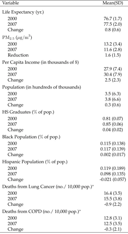
Table 1.1: Summary Characteristics of the 545 Counties Analyzed for the Years 2000 to 2007: (∗), 2005 death rates are used as a proxy for 2007 death rates. COPD denotes chronic obstructive pulmonary disease.

Variable Mean(SD)

Life Expectancy (yr.)

2000 76.7 (1.7) 2007 77.5 (2.0) Change 0.8 (0.6) PM2.5(µg/m3) 2000 13.2 (3.4) 2007 11.6 (2.8) Reduction 1.6 (1.5)

Per Capita Income (in thousands of$)

2000 27.9 (7.4)

2007 30.4 (7.9)

Change 2.5 (2.3)

Population (in hundreds of thousands)

2000 3.5 (6.3) 2007 3.8 (6.6) Change 0.3 (0.6) HS Graduates (%of pop.) 2000 0.81 (0.07) 2007 0.85 (0.06) Change 0.04 (0.02)

Black Population (%of pop.)

2000 0.115 (0.138)

2007 0.117 (0.139)

Change 0.002 (0.017)

Hispanic Population (%of pop.)

2000 0.119 (0.189)

2007 0.098 (0.135)

Change -0.021 (0.057)

Deaths from Lung Cancer (no./ 10,000 pop.)∗

2000 16.4 (3.5)

2007 15.5 (3.8)

Change -0.9 (2.2)

Deaths from COPD (no./ 10,000 pop.)∗

2000 12.8 (3.1)

2007 12.5 (3.5)

Figure 1.2: Cross Sectional and First Difference Plots of PM2.5 vs. Life Expectancy:

Cross-sectional life expectancies plotted vs PM2.5 levels for (A) 2000 and (B) 2007 in

Dataset 1. The slopes of the regression lines correspond to estimates from the simple model: LE=intercept + slope*PM2.5 in both the 2000 and 2007 plots. In the second row

on the left (C) the data are plotted as change in life expectancy vs change inPM2.5over the

period 2000 - 2007. The regression line corresponds to the simple model∆LE =intercept + slope*∆PM2.5 (Model 1 in Table 1.2). (D) On the right is the added variable plot for

Figure 1.2 (Continued) 5 10 15 20 25 70 75 80 PM2.5 Level - 2000 (µg/m3₎ Li fe Exp ect an cy, 2 00 0 (yr) A 5 10 15 20 70 75 80 85 PM2.5 Level - 2007 (µg/m3₎ Li fe Exp ect an cy, 2 00 7 (yr) B -4 -2 0 2 4 6 8 -3 -2 -1 0 1 2 3 4 Reduction in PM2.5, 2000 - 2007 C ha ng e in L ife Exp ect an cy, 2 00 0 - 20 07 C -0.4 -0.2 0.0 0.2 0.4 -2 -1 0 1 2

Reduction in PM2.5 from 2000 - 2007 | Model 3

C ha ng e in L ife Exp ect an cy fro m 20 00 - 20 07 | Mo de l 3 D

Table 1.2 summarizes estimated regression coefficients for the association between changes inPM2.5 and changes in life expectancy for 545 counties for 2000 to 2007 for

se-lected regression models. When controlling for changes in all available socioeconomic and demographic variables as well as smoking prevalence proxy variables (Model 3), a

10µg/m3 decrease in PM2.5 was associated with an estimated mean increase in life

ex-pectancy of 0.35 years (SE= 0.16 years, p = 0.033). The estimated effect ofPM2.5 on life

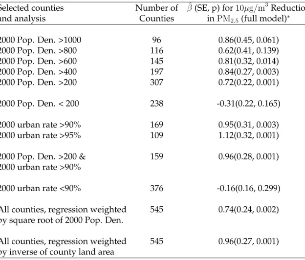
expectancy was consistent across models adjusting for various patterns of potentially con-founding variables (e.g. Models 2 & 3). Models 4 - 8 of Table 1.2 show the results for select stratified and weighted regressions. In counties with a population density greater than 200 people per square mile, a10µg/m3 decrease inPM2.5was associated with an

in-creased life expectancy of 0.72 (0.22 years,p <0.01) (Model 5), compared with -0.31 years (0.22 years,p = 0.165) in counties with less than 200 people per square mile (P difference

<0.01). In counties whose proportion of urban residences was greater than 90 percent, a

10µg/m3decrease inPM2.5 was associated with an increased life expectancy of 0.95 (0.31,

p <0.01) (Model 6), compared with -0.16 (0.16 years,p= 0.299) in counties with less than

1.2: Results of Selected Regression Models for County-Level Analysis, 2000 -2007: ( a ) ,Included only counties with lar gest year 2000 population in their respective MSA; ( b ) , Included only counties with a year 2000 population density 200 people per squar e mile; ( c ) , Included only counties with a year 2000 urban rate > 90% ; ( d ) , W eighted by the squar e of the year 2000 population density; ( e ) , W eighted by the inverse of county land ar ea. Estimate for the ef fect of PM 2 . 5 for a 10 µ g / m 3 reduction; change in income is given in thousands of dollars. Changes in LC ASDR and COPD ASDR ar e in the age standar dized death rate for lung cancer and chr onic obstr uctive pulmonary di sease, respectively . V ariable Model 1 Model 2 Model 3 Model 4 a Model 5 b Model 6 c Model 7 d Model 8 e Inter cept 0.82 ± 0.04 1.08 ± 0.08 1.00 ± 0.08 0.97 ± 0.10 0.91 ± 0.11 0.84 ± 0.15 0.79 ± 0.15 0.67 ± 0.15 Reduction in PM 2 . 5 0.14 ± 0.19 0.35 ± 0.17 0.35 ± 0.16 0.30 ± 0.23 0.72 ± 0.22 0.95 ± 0.31 0.74 ± 0.24 0.96 ± 0.28 Change in income − 0.013 ± 0.017 0.017 ± 0.018 0.005 ± 0.018 0.02 ± 0.02 -0.01 ± 0.03 0.03 ± 0.02 0.05 ± 0.02 Change in pop. − 0.13 ± 0.05 0.11 ± 0.05 0.07 ± 0.05 0.06 ± 0.04 0.02 ± 0.04 0.07 ± 0.06 0.34 ± 0.12 Change in HS % − -9.12 ± 1.61 -7.98 ± 1.56 -7.27 ± 1.95 -4.42 ± 2.60 -4.04 ± 3.20 -1.94 ± 3.35 -3.30 ± 3.45 Change in black % − -6.55 ± 2.05 -6.34 ± 1.97 -7.86 ± 3.07 -12.56 ± 3.59 -8.12 ± 2.84 -11.14 ± 3.00 -6.21 ± 2.97 Change in Hisp % − -2.16 ± 0.47 -2.03 ± 0.47 -2.12 ± 0.59 -0.95 ± 0.62 5.28 ± 3.58 -3.25 ± 0.63 -4.57 ± 0.75 Change in LC ASDR − − -0.02 ± 0.02 -0.02 ± 0.02 -0.01 ± 0.05 -0.05 ± 0.05 -0.07 ± 0.02 -0.07 ± 0.03 Change in COPD ASDR − − -0.05 ± 0.01 -0.05 ± 0.02 -0.06 ± 0.03 -0.06 ± 0.05 -0.08 ± 0.02 -0.06 ± 0.02 No. of county units 545 545 545 257 307 169 545 545

When we re-estimated Model 3 of Table 1.2 using the square root of population density as the weight (Model 7), the estimated effect of a10µg/m3 reduction ofPM2.5 on

life expectancy was more than double that observed in our un-weighted analysis (0.74 [0.24] vs. 0.35 [0.16]). When that same model was weighted by the inverse of county land area (Model 8), the effect was nearly triple that of the un-weighted analysis (0.96 [0.27]). Table 1.3 summarizes a number of our stratified and weighted analyses.

Table 1.3: Summary of Selected Stratified Regression Analyses for 545 Counties

(Dataset 1, 2000 - 2007): (∗) Corresponds to the covariate pattern in Model 3 of Table 1.2. Covariates include change in income, change in population, change in proportion of high-school graduates, change in proportion of black population, change in propor-tion of Hispanic populapropor-tion, change in lung cancer mortality rate, and change in COPD mortality rate. Analysis used: SAS 9.2, PROC SURVEYREG, clustered by MSA, using the "weight" statement, and Stata 11.0, REGRESS using the "cluster" option.

Selected counties Number of βˆ(SE, p) for10µg/m3 Reduction

and analysis Counties inPM2.5(full model)∗

2000 Pop. Den. >1000 96 0.86(0.45, 0.061) 2000 Pop. Den. >800 116 0.62(0.41, 0.139) 2000 Pop. Den. >600 145 0.81(0.32, 0.014) 2000 Pop. Den. >400 197 0.84(0.27, 0.003) 2000 Pop. Den. >200 307 0.72(0.22, 0.001) 2000 Pop. Den. < 200 238 -0.31(0.22, 0.165) 2000 urban rate >90% 169 0.95(0.31, 0.003) 2000 urban rate >95% 109 1.12(0.32, 0.001)

2000 Pop. Den. >200 & 159 0.96(0.28, 0.001)

2000 urban rate >90%

2000 urban rate <90% 376 -0.16(0.16, 0.299)

All counties, regression weighted 545 0.74(0.24, 0.002)

by square root of 2000 Pop. Den.

All counties, regression weighted 545 0.96(0.27, 0.001)

by inverse of county land area

We conducted similar analyses for the 211-county dataset for 1980 to 2007 and from 2000 to 2007, the results of which are presented in Tables 4.3 and 4.4 of Appendix D,

respectively. Results for the period from 1980 to 2000 were identical to those reported by Pope et al. (2009).

Figure 1.3 summarizes the point estimates and 95% confidences interval for the effect of a10µg/m3 decrease in PM2.5 on life expectancy for select weighted and

un-stratified regression models in each dataset/time period. Models fitted using Datasets 2 and 3 (left) controlled for changes in income, population, proportion of the population that is black, lung cancer death rate, and COPD death rate, corresponding to Model 4 in eTables 2a,b. Models fitted using Dataset 1 controlled for all available variables and cor-respond to Model 3 in Table 1.2. These estimates were fairly consistent, though estimates corresponding to the counties from Pope et al. (2009) for the period 2000 to 2007 appeared slightly larger than those from other analyses.

Figure 1.3: Effect Estimates and Confidence Intervals for the Effect of a10µg/m3 De-crease in PM2.5 on Life Expectancy: Estimates A and B were obtained from Dataset 3;

Estimate C was obtained from Dataset 2. Estimates A, B, and C were adjusted for changes in income, population, proportion of the population that is black, lung cancer death rate, and COPD death rate (Model 4, eTables 2a,b). Estimates D, E, and F were obtained from Dataset 1, adjusted for changes in income, population, proportion of high school grad-uates, proportion of the population that is black, proportion of the population that is Hispanic, lung cancer death rate, and COPD death rate (Model 3, Table 1.2). "Pope et al" refers to Pope et al. (2009).

Figur e 1.3 (Continued) -1.0 -0.5 0.0 0.5 1.0 1.5 2.0 2.5 Incre ase in Li fe Expect ancy for a 1 0µ g/m 3 D ecre ase in PM 2.5 A B C D E F A: MSA-l eve l PM; 1 98 0 - 20 07 , 2 11 co un tie s in cl ud ed in Po pe e t a l B: MSA-l eve l PM; 2 00 0 - 20 07 , 2 11 co un tie s in cl ud ed in Po pe e t a l C : MSA-l eve l PM; 1 98 0 - 20 00 , 2 11 co un tie s exa ct ly as re po rt ed in Po pe e t a l D : C ou nt y-l eve l PM; 2 00 0 - 20 07 , 5 45 co un tie s E: C ou nt y-l eve l PM; 2 00 0 - 20 07 , 1 13 co un tie s in cl ud ed in Po pe e t a l F : C ou nt y-l eve l PM; 2 00 0 - 20 07 , 4 32 co un tie s no t i ncl ud ed in Po pe e t a l

In the analyses stratified by sex, the estimated effect of a 10µg/m3 reduction in

PM2.5 for the covariate pattern corresponding to Model 3 of Table 1.2 was an additional

0.59 (0.17) years of life expectancy for women and 0.08 (0.20) years for men (P difference = 0.027). Differences by sex were also observed in stratified and weighted models, although with less precision. Sex differences were smaller in the most urban counties (urban rate

> 90%). Similar results were observed for the period 1980 to 2000 in Dataset 2. Sex-specific results are presented in Table 1.4.

Table 1.4: Comparison of Results of Select Models for Males vs. Females (Dataset 1, 2000 - 2007): (∗_{) Covariates include change in income, change in population, change in} proportion of high-school graduates, change in proportion of black population, change in proportion of Hispanic population, change in lung cancer mortality rate, change in COPD mortality rate. Analysis used: SAS 9.2, PROC SURVEYREG, clustered by MSA, using the "weight" statement, and Stata 11.0, REGRESS using the "cluster" option. (†) Indicates that the estimate for males was statistically significantly different than the estimate for females for the model specified in that row.

Selected counties Males:βˆ(SE, p) for10µg/m3 Females: βˆ(SE, p) for10µg/m3

and analysis Dec. inPM2.5(full model)∗ Dec. inPM2.5(full model)∗

All counties 0.08(0.20, 0.681)† 0.59(0.17, 0.001)†

2000 Pop. Density > 200 0.44(0.25, 0.084) 0.85(0.24, 0.001)

2000 Pop. Density < 200 -0.55(0.27, 0.043) -0.06(0.24, 0.805)

2000 urban rate > 90% 0.81(0.37, 0.033) 1.07(0.28, <0.001)

2000 urban rate < 90% -0.44(0.20, 0.025) 0.08(0.19, 0.664)

All counties, regression 0.57(0.29, 0.047) 0.87(0.22, <0.001)

weighted by square root of 2000 Pop. Den.

All counties, regression 0.74(0.30, 0.013) 1.14(0.30, <0.001)

weighted by inverse of county land area

Effect estimates were not highly sensitive to the inclusion of the estimated change in smoking prevalence. Table 1.5 summarizes the results for the inclusion/exclusion of the smoking prevalence variable across several models. For example, when Model 3 in Table 1.2 was re-estimated for the 383 counties with matching smoking prevalence data,

a reduction of10µg/m3 was associated with an increase in life expectancy of 0.49 (0.19) years without including change in smoking prevalence in the model, and 0.47 (0.19) when including those changes. Similar results for smoking were observed in our stratified and weighted models, as well as in our models for men and women separately.

T able 1.5: Comparison of PM 2 . 5 Ef fect Estimates from Selected Models for Inclusion of Smoking V ariable V ersus No In-clusion of Smoking V ariable: Covariates include change in income, change in population, change in high-school graduates, change in pr oportion of black population, change in pr oportion of Hispanic population, change in lung cancer mortality rate, change in COPD mortality rate. Analysis used: SAS 9.2, PROC SUR VEYREG, cluster ed by MSA, using the "weight" statement, and Stata 11.0, REGRESS using the "cluster" option. Selected counties and analysis No. Counties Full model, with smoking: Full model, no smoking: ˆβ(SE, p) per 10 µ g / m 3 PM 2 . 5 ˆ_β(SE, p) per 10 µ g / m 3 PM 2 . 5 All Counties 383 0.47(0.19, 0.013) 0.49(0.19, 0.011) 2000 population density (persons per squar e mile) >800 110 0.52(0.43, 0.230) 0.53(0.43, 0.221) >600 139 0.68(0.30, 0.028) 0.68(0.30, 0.027) >400 187 0.71(0.26, 0.007) 0.70(0.25, 0.007) >200 272 0.67(0.22, 0.003) 0.65(0.22, 0.004) <200 111 -0.50(0.30, 0.100) -0.39(0.30, 0.193) 2000 urban rate >90% 157 0.76(0.28, 0.009) 0.76(0.28, 0.008) >95% 101 1.01(0.31, 0.002) 0.98(0.32, 0.003) <90% 226 -0.14(0.20, 0.483) -0.13(0.20, 0.513) 2000 population density & 2000 urban rate >200 & 100 0.95(0.32, 0.004) 0.93(0.32, 0.005) >90% Regr ession weighted by squar e root of 383 0.77(0.24, 0.002) 0.76(0.25, 0.003) 2000 population density (All counties) Regr ession weighted by inverse of 383 0.81(0.26, 0.002) 0.74(0.27, 0.007) county land ar ea (All counties) Sex Men 383 0.20(0.23, 0.389) 0.22(0.23, 0.343) W omen 383 0.71(0.20, 0.001) 0.72(0.20, <0.001)

1.4

Discussion

Data on air pollution and life expectancy from 545 US counties in 2000 and 2007 show that recent declines in PM2.5 to relatively low levels continue to prolong life

ex-pectancy in the US. These benefits are largest among the most urban and densely pop-ulated counties. These associations were estimated controlling for socioeconomic and demographic variables as well proxy variables for and direct measures of smoking preva-lence.

In previous studies, a 10µg/m3 decrease inPM2.5 has been associated with gains

from 0.42 to 1.51 years of life expectancy{Tainio et al. (2007); Pope et al. (2009)}. Here, a decrease of10µg/m3 inPM2.5 was associated with an increase in life expectancy of 0.35

(0.16) for 545 counties for the period from 2000 to 2007. An increase in life expectancy of 0.56 (0.19) was estimated for the same 211 counties included in the Pope et al. (2009) anal-ysis but extended to the period 1980 to 2007. The estimated effect in those 211 counties from 2000 to 2007 was equal to 1.00 (0.32). Stratified and weighted analyses within the 545 counties from 2000 to 2007 yielded larger estimates between 0.72(0.22) and 1.12(0.32) - broadly in agreement with those previously reported.

From 2000 to 2007, the average increase in life expectancy across the counties in this study was 0.84 years, and the average decrease inPM2.5 in those same counties was

1.56µg/m3. While PM2.5 reductions presumably account for some of the improvements

in life expectancy over this period, it is only one of many contributing factors. Other factors may include improvements in the prevention and control of the chronic diseases of adulthood, particularly cardiovascular diseases (CVD) and stroke {Yeh et al. (2011); Shrestha (2005)}, and changes in the risk factors associated with them, including medical advances, declines in smoking, and decreases in blood pressure and cholesterol {Shrestha (2005)}. Given the well-established link between air pollution and CVD mortality{Pope et al. (1995, 2002, 2004)}, and changes in other CVD risk factors, issues of multicausality and competing risk make it difficult to quantify exactly the changes in life expectancy

attributable to reductions inPM2.5. However, if we consider one of our more conservative

effect estimates (Model 3, Table 1.2) the1.56µg/m3 reduction inPM2.5 accounts for about

0.055 years (1.56×0.0354) of additional life expectancy, or roughly7% of the increase in life expectancy. Using the estimate from our most urban counties (Model 6, Table 1.2), the increase in life expectancy attributable to the average reduction inPM2.5 was 0.148 years

(1.56×0.095), or as much as18%of the total increase.

An interesting aspect of this study was how pronounced thePM2.5 effect was for

the original 211 counties from 2000 to 2007. Given that they were originally selected sim-ply on the availability of matching pollution data, what is special about these counties that results in larger estimates of the effect ofPM2.5 on life expectancy? The stratified and

weighted analyses suggest plausible explanations. For instance, the 211 counties were all in metropolitan areas, and the stratified analyses suggest that the effect ofPM2.5 on life

expectancy is greatest in the most urban counties. One possible reason is that the com-position of PM2.5 is different in urban areas {Louie et al. (2005)}, causing PM2.5 to have

a larger health impact. Another possibility is the "nonmetropolitan mortality penalty" -the recent phenomenon in which mortality rates are higher in rural compared with urban areas {Cossman et al. (2010)}. While it is not clear why the mortality gap between metro and non-metro areas has widened, some hypotheses include greater improvements in standards of care in metro areas, changes in uninsurance rates, changes in disease inci-dence, and changes in health behaviors {Cossman et al. (2010)}. These, however, would be valid explanations only if they occurred at different rates in metropolitan areas com-pared with rural areas. If so, then perhaps failure to include variables that captured one or more of these differences could explain the different estimates of the effect ofPM2.5 on

life expectancy.

Alternatively, metropolitan areas are more densely populated than non-metro ar-eas. Our models that stratified by population density showed that the effect of PM2.5

on life expectancy is greatest in the most densely populated study areas (those with a population density of at least 200 people per square mile) - possibly suggesting a role

for differential exposure misclassification. That is, in densely populated areas, it is more likely that any two people from the same area are exposed to the same level ofPM2.5 with

perhaps less exposure misclassification. This possibility was supported in our models weighted by the square root of population density and the inverse of land area, which placed more weight on the most densely populated counties and the smallest counties. In these models the effect of a 10µg/m3 decrease in PM2.5 on life expectancy was much

larger than the equivalent un-weighted analysis.

Another interesting finding was the difference in the effect of changes in PM2.5

on men and women. Findings in the literature regarding the effects of air pollution by sex for long-term exposure have been mixed. Studies using the ACS and Harvard Six-Cities cohorts show no significant difference in pollution-related mortality between men and women {Dockery et al. (1993); Pope et al. (1995); Krewski et al. (2000); Pope et al. (2002, 2004); Laden et al. (2006)}. Studies using a Medicare cohort have reported different effects by age and region, but did not stratify by sex {Eftim et al. (2008); Greven et al. (2011); Zeger et al. (2008)}. In a study using the Adventist Health cohort, Chen et al. (2005) reported a large effect of PM2.5 on fatal coronary heart disease (CHD) in women

but no association in men. Similarly, in separate studies, Ostro et al. (2010) using a cohort of women (California Teachers’ Study), reported associations between particulate matter and cardiovascular mortality, while Puett et al. (2011) using a cohort of men (Male Health Professionals), found no association with all-cause mortality or fatal CHD. For our main analysis using all 545 counties, we find a larger effect ofPM2.5on women, suggesting that

reductions in PM2.5 are more beneficial to gains in life expectancy for women. Models

fitted using data for the period from 1980 - 2000 as in Pope et al. (2009) showed simi-lar results. Future work should investigate more thoroughly the possibility of different

PM2.5-mortality associations for men versus women.

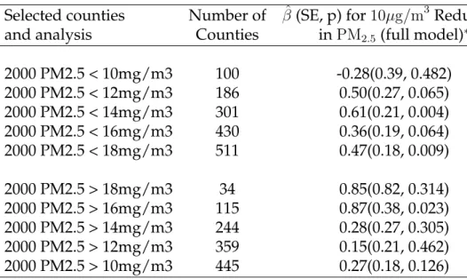
One factor that appeared to play no role in thePM2.5 and life expectancy

relation-ship, however, was baselinePM2.5 level. This is in agreement with the findings by Pope

density, urban rate, and land area, this is not due to these areas having a higher or lower baselinePM2.5 level. Furthermore, this finding suggests that there is no clear threshold

below which further reductions inPM2.5levels provide no benefit (eAppendix, eTable 3).

The fact that our results were not sensitive to the inclusion of direct measures of change in smoking prevalence suggests that the estimated gains in life expectancy for a10µg/m3

reduction inPM2.5 are not a result of confounding due to changes in smoking prevalence.

Table 1.6: Summary of Selected Regression Analyses Stratified by BaselinePM2.5

Lev-els for 545 Counties (Dataset 1, 2000 - 2007): (∗)Corresponds to the covariate pattern in Model 3 of Table 1.2. Covariates include change in income, change in population, change in proportion of high-school graduates, change in proportion of black population, change in proportion of Hispanic population, change in lung cancer mortality rate, and change in COPD mortality rate. Analysis used: SAS 9.2, PROC SURVEYREG, clustered by MSA, using the "weight" statement, and Stata 11.0, REGRESS using the "cluster" option.

Selected counties Number of βˆ(SE, p) for10µg/m3Reduction

and analysis Counties inPM2.5 (full model)∗

2000 PM2.5 < 10mg/m3 100 -0.28(0.39, 0.482) 2000 PM2.5 < 12mg/m3 186 0.50(0.27, 0.065) 2000 PM2.5 < 14mg/m3 301 0.61(0.21, 0.004) 2000 PM2.5 < 16mg/m3 430 0.36(0.19, 0.064) 2000 PM2.5 < 18mg/m3 511 0.47(0.18, 0.009) 2000 PM2.5 > 18mg/m3 34 0.85(0.82, 0.314) 2000 PM2.5 > 16mg/m3 115 0.87(0.38, 0.023) 2000 PM2.5 > 14mg/m3 244 0.28(0.27, 0.305) 2000 PM2.5 > 12mg/m3 359 0.15(0.21, 0.462) 2000 PM2.5 > 10mg/m3 445 0.27(0.18, 0.126)

Unlike previous cross-sectional analyses {Evans et al. (1984); Özkaynak and Thurston (1987)}, we were able to estimate the association between county-specific tem-poral changes in PM2.5 levels and county-specific temporal changes on life expectancy

adjusted by temporal changes in several potential confounding factors. By looking at within-county temporal changes, we reduce the potential bias due to unmeasured con-founding. Further, by estimating clustered robust standard errors at the MSA level, we took a conservative approach in accounting for potential spatial correlation between neighboring counties.

Our analysis has the strengths of using some of the largest available datasets, and applying relatively simple analyses. Additionally, we improved on the original analysis by constructing a dataset withPM2.5measured at the county level, in contrast to the more

coarse MSA-level readings used in previous studies {Pope et al. (2002, 2009)}.

The analysis is limited, however, in its ability to control for all potential unmea-sured confounding. Additionally, in comparing selected years, we do not fully exploit potentially informative data between those years. Furthermore, sophisticated analyses of the U.S. Medicare population by Greven et al. (2011) did not observe associations between "local" trends inPM2.5levels and "local" trends in mortality in 814 zip code level locations

in the U.S. for the period 2000 - 2006. "Local" trends were defined as the difference be-tween monitor-specific trends and national trends. The Medicare cohorts, however, con-sisted only of people age 65 and older, whereas our life expectancy calculations integrate over all ages. Also, other studies using Medicare based cohorts have found significant associations betweenPM2.5 and overall mortality {Eftim et al. (2008); Zeger et al. (2008)}.

Future work is needed to investigate whether these differences among studies are due to differences in statistical models, data sources, or populations studied.

It is also worth considering whether life expectancy was the most appropriate out-come to consider in our model. Because life expectancies are calculated from age-specific mortality rates, perhaps a model with age-specific mortality rates as the outcome would be more appropriate, allowing the age groups most affected byPM2.5exposure to be

pin-pointed precisely.

In summary, our study reports strong evidence of an association between recent further reductions in fine-particulate air pollution and improvements in life expectancy in the United States, especially in small, densely populated urban areas.

A Closer Look at Exposure Decomposition in Long-term

Air Pollution Studies: A Distributed Lag Approach

Andrew W. Correia and Francesca Dominici

Department of Biostatistics

Harvard University

2.1

Background

In the environmental epidemiology literature, there has been a great deal of work on assessing the impacts of air pollution exposure on various health outcomes. These studies range from short-term daily time-series studies {Dominici et al. (2002, 2003)}, to long-term cohort studies {Pope et al. (1995); Dockery et al. (1993)}, to long-term popula-tion based studies {Pope et al. (2009); Correia et al. (2013)}. Due to the nature of the re-search question of interest and the data available to rere-searchers to answer those questions, the majority of these studies are observational. In general, caution is urged when inter-preting parameter estimates from observational studies, as it is very difficult to properly control for every potential confounder (measured and unmeasured) in an observational study {Christenfeld et al. (2004); Greenland and Morgenstern (2001)}. Therefore, a major concern in environmental epidemiology is bias due to residual confounding, and indeed in both long-term and short-term studies, some critics argue that the estimated effect es-timates of air pollution on mortality and morbidity are unreliable due to the difficulty of fully controlling for all potential confounders {Vedal (1997); Moolgavkar (1994, 2005)}.

Recent work by Janes et al., 2007 and Greven et al., 2011 has attempted to overcome issues of residual confounding by decomposing the air pollution exposure variable into a "local" term and a "global" term, where under certain assumptions, differences in the estimated effects of the "local" and "global" terms implies unmeasured confounding. The approach taken in these two papers has been somewhat controversial, as the models fitted via the exposure decompostion approach have estimated a null effect of air pollution on mortality at the "local" level - quite a contrast to the majority of literature on the subject. However, a thorough investigation of the modeling approach in Janes et al., 2007 and Greven et al., 2011 and a discussion as to why the results in those papers stand in contrast to the majority of the literature on air pollution and mortality has, to our knowledge, not been undertaken. The outline of this paper is as follows: 1) We will begin by focusing on the simpler approach presented in Janes et al., 2007, and discussing its methodology and modeling assumptions; 2) we illustrate the implications of those modeling assumptions

via simulation studies; 3) we then discuss the approach in Greven et al., 2011, showing how the modeling assumptions in that paper relate to those in Janes et al., 2007, and also how the simulation results apply to the Greven model; 4) we propose a model that is a combination of the Janes and Greven models, which also integrates a distributed lag on the "local" exposure term to more adequately model the temporal relationship between

PM2.5and mortality; and 5) we close with a discussion.

2.2

Overview of Methodology and Modeling Assumptions

In Janes et al., 2007, the authors’ aim is to estimate the effect ofPM2.5on mortality

in 113 US counties from 1999 to 2002 in the Medicare population. A particular county’s monthlyPM2.5level is calculated as the average ofPM2.5over the preceding year - that is,

the averagePM2.5 level over the past 12 months, including the current month. Mortality

counts in a given month for any county are simply the sum of the number of deaths in that county for the given month; these monthly counts are not given by an average of mortality counts over the preceding year. The authors then stratify individuals into one of six different age-sex strata. It is assumed that the causal model for the effect ofPM2.5

on mortality in each age-sex stratum is given by:

logE(Y_tc) = log(N_tc) +δc₀+δ1PMct, (2.1)

where Yc

t and Ntc are the mortality counts and number of people at risk,

respec-tively, for each countycand montht; theδc

0 are county-specific random intercepts; andδ1

is the association between month-to-month variation inPMc_t and month-to-month varia-tion in mortality.

Because estimates from Model 2.1 are likely to be confounded by variables trend-ing in a similar fashion to PM2.5 and mortality, Janes and colleagues introduce another

con-founding is addressed, at least in part, by a smooth function of time. Specifically:

logE(Y_tc) = log(N_tc) +β₀c+β1PMct+s(t;d), (2.2)

whereβc

0 andβ1 are defined analogously to δc0 andδ1, respectively, and s(t;d)is a

natural cubic spline withddegrees of freedom. From Model 2.2, Janes et al., 2007 propose:

logE(Y_tc) = log(N_tc) +ηc₀+η1PMd_t+η₂(PMc_t−PMd_t) +s∗(t;d−1), (2.3)

where PMdt is the annual average in PM2.5 for month t across all counties and

s∗(t;d−1)is orthogonal to bothPMd_tandPMc_t.

Predicted values from Models 2.2 and 2.3 are equivalent. However, Janes et al., 2007 point out that because Model 2.3 estimates the association betweenPM2.5 and

mor-tality at both a national scale and a local scale, we are able to detect unmeasured con-founding via large differences between the estimates ofη1andη2- if there is no

confound-ing or measurement error,η1 and η2 should be equal; if there is confounding, it is more

likely to be at the global-level (η1) than at the local level (η2). Additionally, the authors

state that the random, county-specific intercepts in the model control for unmeasured county-specific characteristics that do not vary with time (i.e. they control for unmea-sured spatial confounding).

In summary, the modeling assumptions given in Janes et al., 2007 (and, generally, in Greven et al., 2011 as well) are as follows:

1. The true causal model for the effect ofPM2.5on mortality is given by Model 2.1.

2. Absent confounding and measurement error, if the causal link between mortality andPM2.5is given by Model 2.1 then the estimates ofη1andη2in Model 2.3 should

3. Estimates should not be biased as a result of spatial confounding due to the inclu-sion of random, county-specific intercepts.

4. Mortality in montht has a causal relationship withPM2.5 levels averaged over the

past twelve months up to and includingt.

5. The estimate ofη2 is less likely to be confounded than the estimate ofη1.

Since one cannot ever know the true underlying causal model, we assume that item 1 is correct. Further, for reasons outlined in Janes et al., 2007 and Greven et al., 2011, we will proceed under the assumption that item 5 is correct as well. Then, given the proposed causal model (2.1), we test assumptions 2, 3 and 4 via simulation in the following section. Because the model in Greven et al., 2011 is much more computationally intensive, we conduct our simulations based on the model presented in Janes et al., 2007 and then discuss how those simulation results relate to the Greven model.

2.3

Simulation Study

2.3.1

Equality of

η

and

η

To test assumption 2, we first simulated data based on Model 2.1 withδ1 = 0.009

and withδc₀ = −5.75for allcusing realPM2.5 and population data - the samePM2.5 and

population data used in Greven et al., 2011, where it is described in more detail. We then analyzed the simulated data with Model 2.3 to be sure that we do indeed observe

η1 ≈ η2 in this simplest scenario. Note that because we assumeδ0c = −5.75for all c, we

fit Model 2.3 with a fixed intercept (η0) instead of a random intercept (ηc0). This is only to

improve computational speed and has no impact on assessing the validity of assumption 2. Also note that we set δ1 = 0.009, as this corresponds roughly to the average estimate

across strata in the non-decomposed model in Janes et al., 2007, and it is also roughly the average effect-estimate of a number of short-term studies summarized in Table 1 of Pope and Dockery, 2006. As this study explores mostly temporal variability, much like many

short-term studies, we believe this is a realistic, though perhaps conservative value forδ1

given the results in the literature for other long-term studies {Table 2, Pope and Dockery, 2006}. Throughout this paper, the degrees of freedom parameter for the cubic spline in Models 2.2 and 2.3,d, is taken to be16as in Janes et al., 2007.

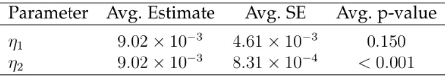
Results under this basic simulation assuming no confounding are given in Table 2.1 below. Indeed, though estimates ofη1 are a bit more variable than those ofη2, we see

that, on average,η1 ≈η2 when there is no confounding.

Table 2.1: Performance of Model 2.3 Under the Assumption of no Confounding: η1 is

the global parameter andη2is the local parameter.

Parameter Avg. Estimate Avg. SE Avg. p-value

η1 9.02×10−3 4.61×10−3 0.150

η2 9.02×10−3 8.31×10−4 <0.001

Temporal Confounding

We then simulate under Model 2.1 again, but with the addition of a confounder,

Ut, trending only at the national level. That is, Ut was generated to be correlated with

both the outcome andPMd_t, butU_tis not correlated with(PMc_t−PMd_t). Outcome data was generated via the following model:

logE(Y_tc) = log(N_tc) +δc₀+δ1PMct +δ2Ut, (2.4)

whereδ2 = 0.15. Simulated data is again modeled under Model 2.3. Results are

summarized in Table 2.2 below:

Table 2.2: Performance of Model 2.3 Under the Assumption of Global-scale Temporal Confounding: η1 is the global parameter andη2is the local parameter.

Parameter Avg. Estimate Avg. SE Avg. p-value

η1 8.44×10−2 7.52×10−3 <0.001

η2 9.09×10−3 1.38×10−3 <0.001

true effect. The same is true when outcomes are generated from a model with a positive interaction effect betweenPMd_tandU_t.

Spatial Confounding

In this section we test assumption 3 - that the estimates ofη1 andη2 should not be

impacted by confounders that do not vary with time to due to the inclusion of location-specific intercepts. Thus, consider a new confounder,Uc_{, that only varies spatially and is}

constant across time. Outcome data is generated by:

logE(Y_tc) = log(N_tc) +δ₀c+δ1PMct+δ2Uc, (2.5)

whereδc₀ =−6.25for allc,δ1 = 0.009, andδ2 =−0.15. Ucis generated such that

Corr(Uc,PMc)≈0.25, andPMc= (1/T)P

tPM c

t ∀c. We again model this outcome data

via Model 2.3, but this time allowing for estimation of location-specific intercepts,η₀c. Results are summarized in Table 2.3 below.

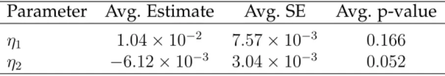
Table 2.3:Performance of Model 2.3 Under the Assumption of Spatial Confounding: η1

is the global parameter andη2 is the local parameter.

Parameter Avg. Estimate Avg. SE Avg. p-value

η1 1.04×10−2 7.57×10−3 0.166

η2 −6.12×10−3 3.04×10−3 0.052

We can see that, despite allowing for the estimation of location-specific intercepts, the average estimate of η2 is severely biased, while the estimate of η1 is only slightly

biased, suggesting that assumption 3 - that estimates are not susceptible to spatial founding - does not hold. In other words, in the presence of unmeasured spatial con-founding, even if we introduce into the model a county-specific random intercept, the estimate of the local effect can be severely biased.

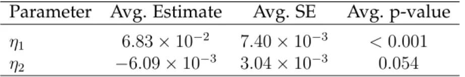
Spatial and Global Temporal Confounding

In this section, we assume there exists both a spatial confounder,Uc_{, and a "global"}

temporal confounder,Ut. Outcome data is generated by:

logE(Y_tc) = log(N_tc) +δc₀+δ1PMct+δ2Uc+δ3Ut, (2.6)

whereδc₀ =−8.22for allc,δ1 = 0.009,δ2 =−0.15, andδ3 = 0.15. ConfoundersUcandUt

are generated such thatCorr(Uc,PMc)≈0.25, andCorr(Ut,PMt)≈0.3. Outcome data is

again modeled via Model 2.3, again allowing for the estimation of location-specific intercepts,ηc

0. Results are summarized in Table 2.4 below:

Table 2.4:Performance of Model 2.3 Under the Assumption of Spatial and Global-scale Temporal Confounding: η1 is the global parameter andη2 is the local parameter.

Parameter Avg. Estimate Avg. SE Avg. p-value

η1 6.83×10−2 7.40×10−3 <0.001

η2 −6.09×10−3 3.04×10−3 0.054

Results for the local term,η2, are very similar to the previous case with only spatial

confounding, which is to be expected since the local and globalPM2.5 terms are

orthogo-nal. We also observe that the global term,η1, becomes inflated due to the global temporal

confounder, as in the earlier simulation with only temporal confounding at the global level. Thus, in the case of global temporal confounding together with spatial confound-ing, we observe that both the local and global terms can be quite biased. It is also possible in this situation, since the local and global terms are each affected separately by the

spa-tial and global temporal confounding, that both estimates could similar in magnitude but bothbe biased as a result of different sources of confounding.

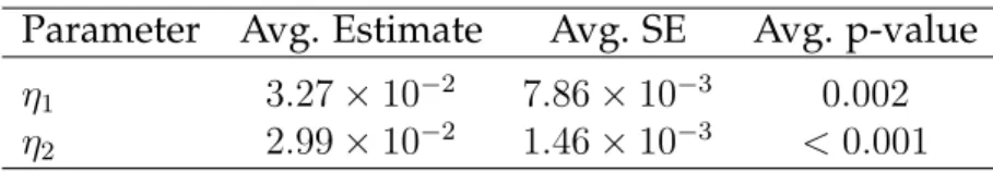
Spatio-temporal Confounding

Now, suppose instead that confounding takes place at the local level and varies with time. Specifically, we generateUc

t to be correlated withPM c

t (Corr(PM c

t, Utc) ≈ 0.25)

and generate outcome data via the following model:

logE(Y_tc) = log(N_tc) +δ₀c+δ1PMct+δ2Utc, (2.7)

again withδ1 = 0.009,δ2 = 0.15, andδc0 =−7.35for allc. Analyzing this data under

Model 2.3 allowing for the estimation of location-specific intercepts yields the following results (Table 2.5):

Table 2.5: Performance of Model 2.3 Under the Assumption of Local Spatio-temporal

Confounding: η1 is the global parameter andη2is the local parameter.

Parameter Avg. Estimate Avg. SE Avg. p-value

η1 3.27×10−2 7.86×10−3 0.002

η2 2.99×10−2 1.46×10−3 <0.001

In this instance, we observe that η1 ≈ η2. Because of this, however, we would

incorrectly assume that the estimates arenotconfounded, though they are, in fact, biased upward - both more than3×higher than the truth,0.009.

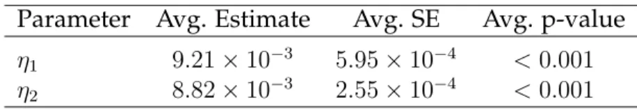
2.3.2

Size of the Window for Averaging Monthly Air Pollution

Two-month Rolling Mean vs 12-month Rolling Mean

In this section, we test the implications of assumption 4 being incorrect. Recall that assumption 4 assumes that mortality at time tis associated with the averagePM2.5 over

the past 12 months. First, we investigate what happens if the true causal relationship betweenPM2.5 and mortality only exists at, say, a two-month window as opposed to the

12-month window assumed in Janes et al., 2007 and Greven et al., 2011.

Consider, again, outcome data generated via Model 2.1 with no confounding and withδ₀candδ1as described above. However, we generate that outcome data withPMct =

(PMc_t,raw + PMc_t−1,raw)/2, where PMc_t,raw is the raw, observed PM2.5 level in county c at

time t, not averaged over any previous or future months’ values. We then model this outcome data using Model 2.3, but withPMc_t = 1

12

P11

i=0PM

c

t−i,raw, as in Janes et al., 2007

and Greven et al., 2011. Results are given in Table 2.6 below:

Table 2.6: Performance of Model 2.3 Under the Assumption of a Mis-specified Rolling Mean: η1is the global parameter andη2 is the local parameter.

Parameter Avg. Estimate Avg. SE Avg. p-value

η1 9.21×10−3 5.95×10−4 <0.001

η2 8.82×10−3 2.55×10−4 <0.001

Surprisingly, the mis-specifiedPMc_t that incorporates information from ten extra, uninformative months actually performs quite well, andη1 and η2 are indeed nearly the

same and very near the truth of0.009. As in the previous section, the estimate of the local term,η2, was very robust to the inclusion of a “global" confounder, and remained

unbi-ased. Thus, it appears that mis-specifying the length of the rolling mean is not terribly serious offense with regards to accurately estimating the regression coefficients.

Generating Data with a Distributed Lag

Suppose now that the association betweenPM2.5 and mortality is best captured by

a distributed lag model:

logE(Y_tc) = log(N_tc) +δ₀c+

q

X

l=0

toq. In other words, we assume not only that pollution at timetaffects mortality at time

t, but also that pollution levels at timest−1, t−2, . . . , t−qimpact mortality at timet. Model 2.8 above is known as anunconstraineddistributed lag model - one simply

calculates the lagged values of the exposure and plugs them directly into the regression. If the successive values of the exposure are highly correlated, however, estimates of the theδl’s will be very unstable. To overcome this, it’s useful to constrain theδl’s to increase

efficiency of the estimated lag parameters {Schwartz (2000)}. The most popular approach for constraining the regression coefficients is that of Almon, 1965, where the shape of the distributed lag (see figure below for an example) is fit by some polynomial function of degreep. Alternative choices include constraining the shape of the distributed lag with a piecewise natural cubic spline {Corradi and Gambetta, 1976; Zanobetti et al., 2000}, B-splines of an arbitrary degree, or simple moving averages (as was done in Janes et al. (2007) and Greven et al. (2011)), among others {Gasparrini et al. (2010)}.

Now, let’s suppose that the relationship betweenPM2.5 and the relative risk (RR)

of mortality is described by Figure 2.1. Here, we see some initial mortality displacement, or "harvesting" {Schwartz (2001)}, followed by a (only partially pictured) sustained but modest long-term increase in the RR of mortality after around 13 months.

We generated outcome data under Model 2.8 so that the relationship between

PM2.5 and mortality is described by Figure 2.1, with δ0c constant across all c; we then

fit that data under Model 2.3. Results are summarized below:

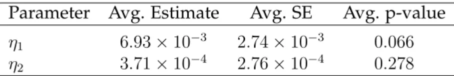
Table 2.7: Performance of Model 2.3 Under the Assumption of an Underlying Lagged

Relationship: η1 is the global parameter andη2is the local parameter.

Parameter Avg. Estimate Avg. SE Avg. p-value

η1 6.93×10−3 2.74×10−3 0.066

η2 3.71×10−4 2.76×10−4 0.278

In this simulation, we observeη1 >> η2 (more than18×greater). However, there

is no confounding under this simulation, only a distributed lag where the relationship is given by that of Figure 2.1. Model 2.3 does relatively well in capturing the overall

Figure 2.1: Example of Distributed Lag Relationship and Corresponding Cumulative Distributed Lag: Plots of the relative risk of mortality by lag (a) and cumulative relative risk of mortality by lag (b).

Figure 2.1 (Continued)

(a) Relative risk for a10µg/m3increase inPM2.5by lag

RR over the entire 15-month lag (estimated, on average, to be 6.36 × 10−4_{), but it is}

unable to tell us anything about the large bump in the RR of mortality that exists out until just after 5 months. Thus, if the true relationship betweenPM2.5 and mortality over

time is given by a similar distributed lag, the model specified by Janes et al., 2007 - and the accompanying assumptions for that model - would lead to a conclusion that the estimates are confounded, and that, on average, the local effect estimate is not statistically significant. The model would also fail to identify any bumps in mortality that are a function of mortality displacement over the duration of the lag window.

2.4

Extensions to Greven et al

In Greven et al., 2011, the authors begin with individual-level data, and wish to fit the proportional hazards model:

hc(a, t) = hc(a)exp(xc_tβ),

wherehc_{(a, t)denotes the hazard of dying at ageaand timetfor locationc,h}c_{(a)is a}

location-specific baseline hazard, andxc

tis averagePM2.5 exposure for countycat timet

as described above. Ageatakes on integer values from65to89; subjects age90or older are pooled into the same age group,I(a≥90). Due to computational constraints given the size of the data set (18.2 million individuals across 814 different locations), the authors instead opt to fit the log-linear regression model:

logE(Y_atc) = log(N_atc) + log(hc(a)) +xc_tβ, (2.9)

Laird and Olivier (1981)}. From Eq. 2.9, the authors then propose a model wherexc t is

decomposed:

logE(Y_atc) = log(N_atc) + log(hc(a)) + (xc_t−x¯t−x¯c+ ¯x)β1+ (¯xt−x¯)β2, (2.10)

where the goal is to, as in Janes et al., 2007, identify unmeasured confounding via large differences between the estimates ofβ1 andβ2. Estimating the parameters in Model 2.10

directly is computationally demanding, as there are still roughtly 1.4 million

observations across all locations and times combined, and there is a need to directly estimate the log-hazardlog(hc_{(a))for all 814 locations,c, separately to control for spatial}

confounding. Thus, the model is fitted using a backfitting algorithm {Buja et al. (1989)}, which iterates betweenStep 1: estimating thePM2.5effect for all locations -β1 andβ2

-including the previous iteration’s estimated hazard as an offset, andStep 2:separately estimating the log-hazard function for each location with(xc_t−x¯t−x¯c+ ¯x)β1+ (¯xt−x¯)β2

as an offset.

Model 2.10 is very similar to Model 2.3; all of the simulation results above for the model in Janes et al. apply to this model except for one: Because a log-hazard function is estimated separately for each location via the backfitting algorithm, the location-specific hazard functions eliminate all purely spatial variation, which means that the estimate of

β1 can not be confounded by variables that vary only across locations. This approach is

similar to fitting a separate model for each location, c, and then pooling the βc

1 estimates

across all locations; clearly no location-specific variables can be identified in that case because they would be absorbed into the intercept term since they are constant over time.

Consider the following – for any fixed time point,t=T, Model 2.10 is given by:

logE(Y_a,tc_=T) = log(N_a,tc _=T) + log(hc(a)) + (xc_t=T −x¯t=T −x¯c+ ¯x)β1+ (¯xt=T −x¯)β2. (2.11)

logE(Y_a,tc_=T) = log(N_a,tc _=T) + log(hc(a)) + (xc_t=T −x¯c−∆¯xt=T)β1. (2.12)

However, this model contains two terms that are constant with respect toc– the location specific indicator,log(hc_{(a)), and, becausetis fixed att=T,(x}c

t=T −x¯c−∆¯xt=T)– which

meansβ1is not identifiable. Thus,β1is only estimable via temporal variations, which

means that it is not susceptible to bias via purely spatial confounders. Therefore, the results from the "spatial confounding" and "spatio-temporal confounding" sections above do not apply to the Greven et al., 2011 model.

For some confounderUt

c to bias the local effectβ1, it would have to be associated

with county-specific deviations in both PMc_t and mortality from each of their respective national trends. An example would be if communities which showed larger decreases inPM2.5 than the national average also consistently showed larger decreases in smoking

rates than the national average, and vice versa {Greven et al., 2011}. While possible, this type of confounding is certainly less likely than variables trending in a similar fashion on the national level, which is why these analyses focus more on the local effect estimates.

Another key distinction to make between the two models is the decomposition of PMc_t in each model. In Janes et al. (2007), the modeling approach decomposes the exposure xc_t into (xc_t−x¯t)and (¯xt−x¯). In Greven et al., the exposurexct is decomposed

into [(xc_t−x¯t)−(¯xc−x¯)], (¯xt −x¯), and (¯xc −x¯), where (¯xc −x¯) gets absorbed into the

location-specific hazard. Interestingly, while the "local" terms in each model should have similar interpretations {Greven et al., 2011}, it appears that they do not. For the data used by Greven and colleagues, we calculated both exposure decompositions - call(xc

t−

¯

xt) ≡ xJ,local and call [(xct−x¯t)−(¯xc−x¯)] ≡ xG,local. Corr(xJ,local, xG,local) = 0.27 and

Corr(xG,local,PMct) = 0.26, whileCorr(xJ,local,PMct) = 0.98. Clearly, the local term in the

Janes decomposition is more representative of the rawPM2.5levels that we want to make

inference about. Also consider the Table 2.8 below, in which we present the results for our most basic simulation under no confounding, but using the Greven decomposition