Full Terms & Conditions of access and use can be found at
http://www.tandfonline.com/action/journalInformation?journalCode=rbri20
Building Research & Information
ISSN: 0961-3218 (Print) 1466-4321 (Online) Journal homepage: http://www.tandfonline.com/loi/rbri20
Energy use and height in office buildings
Daniel Godoy-Shimizu, Philip Steadman, Ian Hamilton, Michael Donn,
Stephen Evans, Graciela Moreno & Homeira Shayesteh
To cite this article: Daniel Godoy-Shimizu, Philip Steadman, Ian Hamilton, Michael Donn, Stephen Evans, Graciela Moreno & Homeira Shayesteh (2018): Energy use and height in office buildings, Building Research & Information, DOI: 10.1080/09613218.2018.1479927
To link to this article: https://doi.org/10.1080/09613218.2018.1479927
© 2018 The Author(s). Published by Informa UK Limited, trading as Taylor & Francis Group
View supplementary material
Published online: 26 Jun 2018.
Submit your article to this journal
Article views: 175
RESEARCH PAPER
Energy use and height in o
ffi
ce buildings
Daniel Godoy-Shimizua, Philip Steadmana, Ian Hamilton a, Michael Donn b, Stephen Evans a, Graciela Morenocand Homeira Shayestehd
a
UCL Energy Institute, University College London, London, UK;bSchool of Architecture, University of Victoria, Wellington, New Zealand;cLDA Design, London, UK;dDesign Engineering and Mathematics, Faculty of Science and Technology, Middlesex University, London, UK
ABSTRACT
The relationship between energy use and height is examined for a sample of 611 office buildings in England and Wales using actual annual metered consumption of electricity and fossil fuels. The buildings are of different ages; they have different construction characteristics and methods of heating and ventilation; and they include both public and commercial offices. When rising from five storeys and below to 21 storeys and above, the mean intensity of electricity and fossil fuel use increases by 137% and 42% respectively, and mean carbon emissions are more than doubled. A multivariate regression model is used to interpret the contributions of building characteristics and other factors to this result. Air-conditioning is important, but a trend of increased energy use with height is also found in naturally ventilated buildings. Newer buildings are not in general more efficient: the intensity of electricity use is greater in offices built in recent decades, without a compensating decrease in fossil fuel use. The evidence suggests it is likely–although not proven–that much of the increase in energy use with height is due to the greater exposure of taller buildings to lower temperatures, stronger winds and more solar gains.
KEYWORDS
building performance; buildings; CO2emissions; energy; epidemiology; height; multivariate regression; office design; tall buildings
Introduction
Taking the domestic and non-domestic sectors together, the average annual turnover of the UK building stock is only 1% (Jones, Patterson, & Lannon, 2007). Conse-quently, significant improvements are required across both new and existing buildings to meet long-term national emissions-reduction targets. In order to ensure that any decisions about changes to the existing stock or the design of new buildings are made effectively, an understanding is required about the relationships between building characteristics and energy use.
Historically, global trends in high-rise construction have reflected changing technologies, planning policies, architec-tural interests and broader societal concerns (Oldfield, Trabucco, & Wood, 2009). In recent years, the UK has been building taller. In 2015, approximately one-third of the UK’s 100 tallest buildings had been completed in the previousfive years; by 2020, this trend is expected to accel-erate further (Skyscraper Center; http://www.skyscraper center.com/). However, despite perceptions that tall build-ings are necessary to achieve high urban densities, research
has shown that this is not the case. It is often possible to achieve the same densities as tall, freestanding towers with lower-rise buildings designed as slabs, terraces or courtyards (Steadman,2014). Since the turnover of build-ings is so slow, and the need for high-rise is debatable, it is particularly important to examine the impact of built form design choices on energy performance.
This paper examines the energy consumption of offices in England and Wales, using information for 611 buildings, collected from three sources of disaggre-gate data: the Display Energy Certificate (DEC) scheme, the Better Buildings Partnership (BBP) and the London Mayor’s Energy Challenge (EC) databases. The analysis focuses on the impact of building height on electricity and fossil fuel use, as well as emissions.
Energy, height and the external environment of buildings
The structural design of high-rise buildings is typically more complex than low-rise buildings due to the
© 2018 The Author(s). Published by Informa UK Limited, trading as Taylor & Francis Group
This is an Open Access article distributed under the terms of the Creative Commons Attribution License (http://creativecommons.org/licenses/by/4.0/), which permits unrestricted use, distribution, and reproduction in any medium, provided the original work is properly cited.
CONTACT Daniel Godoy-Shimizu d.godoy-shimizu@ucl.ac.uk
Supplemental data for this article can be accessed athttps://doi.org/10.1080/09613218.2018.1479927
increased load effects associated with height (Tamoš ai-tienė& Gaudutis,2013). Consequently, embodied energy intensity increases substantially as buildings get taller (Resch, Bohne, Kvamsdal, & Lohne,2016; Treloar, Fay, Ilozor, & Love, 2001), although this ‘height premium’ can be partly mitigated through design and material choices (Ali & Moon, 2007; Chau, Hui, Ng, & Powell, 2012; Foraboschi, Mercanzin, & Trabucco,2014). Typi-cally, however, embodied energy accounts for only 10– 20% of the overall lifecycle of buildings compared with 80–90% associated with operational energy (Ramesh, Prakash, & Shukla,2010).
Energy consumption in the operation of buildings is determined by a large number of variables, including dis-tinct architectural and engineering design choices, as well as broader factors such as occupancy behaviour and the external environment. Analyzing the drivers of building performance, Baker and Steemers (1994) suggest that building design, including height, can account for a 2.5 times variation in energy use, while the systems and occu-pancy behaviour each account for a 2.0 times variation. This analysis was expanded to consider urban geometry, which was found to account for approximately a 10% vari-ation in energy use (Ratti, Baker, & Steemers,2005).
Other things being equal, the primary direct impact of a building’s height on its energy consumption is through interactions with the external environment.1 Climate changes with altitude, affecting thermal transfer and infiltration rates. For example, external air temperature and wind speed fall and rise with altitude respectively, although the magnitude of change varies with local con-ditions (CIBSE,2006). Access to daylight and solar gains, meanwhile, is determined by the height and location of a building relative to its surroundings. While the effect of each separate factor may be straightforward to estimate, the net impact on energy consumption for any specific building will depend on variables including the installed systems, occupancy behaviour and exposed thermal mass. For example, increased daylight availability will only reduce a building’s demand for artificial lighting if the controls are somehow linked to daylight, and there are no adverse effects that encourage occupants to close blinds, such as excessive glare, solar gains or privacy issues. Many of the studies that consider building height use thermal modelling to estimate the performance of theoreti-cal built forms. Analyzing simple forms introduces the complication that the number of storeys, total floor area and area per floor are interlinked. Parasonis, Keizikas, and Kalibatiene (2012) and Hemsath and Bandhosseini (2015) show that, maintaining total floor area, building height correlates positively with heat loss and modelled residential energy use, largely driven by resulting changes in overall compactness. Significantly, height was found to
have a greater impact on residential energy use than con-struction materials, depending on the climate (Hemsath & Bandhosseini,2015). A small number of studies model the energy performance for case study buildings. Ellis and Torcellini (2005) showed that total heating and cooling energy use in a simple rectangular office skyscraper in Manhattan increases between the lowest and highest
floors. The net increase in energy consumption was rela-tively small (approximately 3% rise between the bottom and top storeys). However, by repeating the analysis mul-tiple times with different model settings, they illustrated that the driving force for this trend was the change in over-shadowing from surrounding buildings, suggesting that a key factor is the relative form of a building compared with its surroundings. This is echoed in a case study in Sin-gapore that estimated that 4.7% of building cooling demand was associated with the relative height of the surrounding buildings (Wong et al., 2011). Similarly, Steemers (2003) notes that in order to minimize energy demand, glazing ratios should reduce considerably between lower and upperfloors, reflecting the variation in local obstructions with height. For London, mean glazing ratios of 38% and 25% are proposed for ground level and at 30 m respectively. While building simulation enables controlled tests to be undertaken, a comparison with empirical data high-lights the difficulty of accounting for factors such as occupancy behaviour (Wright, 2008). Furthermore, assumptions about building characteristics may not be straightforward. For example, a survey of offices in the US and the UK found no correlation between airtight-ness and building age or materials, but found that taller buildings tended to have lower infiltration rates (Emmer-ich & Persily, 1998). The need for actual energy and building data to form the basis of research into the built environment, rather than relying solely on mod-elled energy demand and theoretical building character-istics, is urged by Hamilton et al. (2013) who propose a greater focus on empirical methods such as‘energy epi-demiology’. They highlight the need for large-scale (pre-ferably population-level) analyses to be carried out where possible, and for smaller studies to be undertaken within the context of the overall population. Moreover Gon-çalves and Bode (2011) note that the need to analyze metered energy data is especially pertinent for tall build-ings, where energy reductions can be particularly chal-lenging to achieve.
In recent years, a small number of large-scale studies of disaggregate energy data have been undertaken using publicly available data for the UK (Armitage, Godoy-Shi-mizu, Steemers, & Chenvidyakarn, 2015; Godoy-Shi-mizu, Armitage, Steemers, & Chenvidyakarn, 2011; Hong & Steadman, 2013) and the US (Yalcintas & Aytun Ozturk, 2007). A recent survey, examining the
energy data of schools in England, found no significant variation in energy with height (Hong, Paterson, Mumo-vic, & Steadman,2014). However, this likely reflects the building type, which is predominantly naturally venti-lated and very low-rise (Tian & Choudhary, 2012). In contrast, an analysis of aggregate energy use in London found that domestic gas consumption was higher in areas marked by tall buildings when accounting for other influencing factors (Hamilton et al., 2017). No equivalent variation in domestic electricity use was found. Elsewhere, a study examining the data from a sur-vey of 20 all-electric air-conditioned offices in Hong Kong reveals a 43% increase in mean electricity use inten-sity between buildings below 11 storeys and those above 20 storeys (Lam, Chan, Tsang, & Li, 2004).2 Electrical equipment and heating, ventilation and air-conditioning (HVAC) accounted for the largest absolute increase in mean intensity, rising by 43 and 40 kWh/m2respectively. Interestingly, mean lighting intensity increased by 20% between the shortest and tallest buildings, despite a corre-sponding rise in glazing level and reduction in overshad-ing from surroundovershad-ing buildovershad-ings.
Taken as a whole, the literature highlights the need for further large-scale, empirical examination of the relationship between building height and energy use. While the influence on embodied energy is well under-stood, relatively few studies have examined the impact of height on operational energy. A number of studies have found a positive correlation between energy con-sumption and height. However, many of these rely on modelled, rather than actual, energy data and the empiri-cal studies that do exist typiempiri-cally consider small numbers of buildings. The work reported here is new in consider-ing energy and height, usconsider-ing actual metered energy data, for a large number of buildings.
Structure of this paper
This paper examines the performance of several hundred offices in England and Wales, using disaggregate energy data gathered from three sources. The data were com-bined with other pre-existing information, alongside the results of a desktop survey undertaken by the authors. This combined data set has been analyzed to evaluate how energy use varies with building height.
The paper is structured as follows. The next section summarizes data that were collected and outlines the processing undertaken to produce a unified buildings database. Next, the overall energy performance of the sample is assessed, including the variation with height, and a generalized linear modelling (GLM) is produced. Finally, the results are discussed, with proposals for further work.
Methods
The key underlying requirement for statistical building studies of this nature is actual, metered disaggregate energy-use data, available for a large sample of buildings. A small number of recent studies have analyzed the per-formance of the UK stock in this way, using energy data from DECs (Godoy-Shimizu et al., 2011; Hong et al., 2014). The DEC database is a collection of energy records gathered since 2008 mostly for public buildings in England and Wales, and originally introduced to improve public understanding about energy use in the building stock (Department of Energy and Climate Change (DECC),2013). Aside from unavoidable factors such as human error, using data from a single source ensures that the collection and processing of the under-lying data remains consistent. However, it also means that the analysis will reflect any biases within the original sample. For example, it has been found that public sector offices have different energy profiles compared with pri-vate offices (Department for Business, Energy & Indus-trial Strategy (BEIS), 2016). Consequently, an examination of the DEC database, which is predomi-nantly public, will not reflect the behaviour of the non-domestic stock as a whole. Naturally, the impact of any biases will depend on the area of study. For example, public buildings form a greater proportion of the overall stock and totalfloor area in education than in the office or retail sectors.
For this study, energy data were gathered from three separate sources; the DEC, the BBP and the London Mayor’s EC databases. The BBP is a consortium of pri-vate sector property companies devoted to improving the performance of the commercial building stock. The Mayor’s Energy Challenge was a competition to encou-rage improvements in London’s buildings. It should be noted that while using these sources together may ensure that the analysis covers a wider range of buildings than any individual source, biases will still exist within the overall sample. For example, all three sources skew towards buildings with largefloor areas. Again, the data-bases are each connected with energy saving initiatives. Therefore, the buildings within the sample may tend to be operated with a greater focus on energy performance than the overall office stock. The energy data were orig-inally collected in the periods 2009–14, pre-2011 and 2010–14 for the BBP, DEC and EC respectively.
Within the UK, a single register of disaggregate built form data does not exist. Therefore, the energy data were combined with additional information about the physical and operational characteristics of the sample from several different sources. These can be grouped into two broad categories:
. Existing data
Information was gathered from three sources: the UK government’s database of property information e-PIMS (https://data.gov.uk/dataset/epims), and two websites for tall buildings: Emporis (https://www. emporis.com/) and Skyscraper Center (http://www. skyscrapercenter.com/).
. Additional data collection
Further data were gathered by the authors through an implementation of 3DStock, a comprehensive model of the physical characteristics of buildings in England and Wales and the activities they house, generated using digital maps and property taxation data (Evans, Liddiard, & Steadman,2017). A desktop sur-vey was also carried out using imagery from Google Maps (https://www.google.co.uk/maps) and Bing Maps (https://www.bing.com/maps).
The information gathered from the different sources was originally collected at different times, and for diff er-ent purposes. Consequer-ently, considerable work was
necessary for checking, processing and combining the separatefiles.Figure 1summarizes the approach taken. For full details, see the Appendix in the supplemental data online.
As the basis of the study, the energy data were pro-cessedfirst (step A inFigure 1). Addresses and construc-tion ages were used to match entries associated with the same buildings. Next, each of the additional data sources was matched in turn (step B), and further data collection was undertaken (step C). Due to inconsistencies between thefiles, it was necessary to recheck old matches after each new source was added. For example, two entries might appear to cover separate buildings based on the addresses in the energy data. However, matching with the Skyscraper Center data might reveal that they are actually part of the same building. Finally, the different
files were combined into a single database, using weather correction to adjust for differences in the collection periods for energy data (step D).
Thefinal combinedfile consisted of information for 708 offices across England and Wales. However, the
A. ENERGY DATA
(DECs; BBP; EC)
A1. INITIAL PROCESSING
Remove doubtful and incomplete entries
A2. STANDARDISE
Unify formatting and units between files A3. MATCH DATA
Match between and within files Assign unique refs
B. OTHER DATA
*(e-PIMS; Emporis; Skyscraper Center)
B1. MATCH
Match to energy data Assign unique refs
B2. PROCESS & STANDARDISE Process and unify data to energy data
C. DATA COLLECTION
* (3DStock; Desktop survey)C1. SELECT BUILDINGS Select buildings to be surveyed C2. COLLECT DATA
Run 3DStock
Carry out desktop survey C3. PROCESS
Process results to identify doubtful data
D. FINAL DATABASE
(The high-rise buildings database)
D1. COMBINE
Combine the separate files based on refs D2. FINAL PROCESSING
Check for inconsistencies or doubtful data Weather correction of energy data * After each new dataset is matched, re-check the existing matched data.
Figure 1.Summary of the methodology used to produce thefinal database.
analysis that follows was carried out only on the 611 buildings for which the main heating fuel was identified as not being electricity. References to the‘high-rise build-ings data’ in this paper refer to this cleaned and com-bined final data set, and the analysis that follows was carried out on these data (or subsets of it) rather than on any of the original raw files. Table 1 summarizes the information within thefinal database. Variables in the original data that do not form part of this study are not listed. The desktop survey was designed as part of a broad study of built form and urban density. Conse-quently, several variables were included that were not used in this study. For full details of these, see Appendix in the supplemental data online.
Results and discussion
This section examines the energy performance of the buildings within the high-rise database. The analysis is presented in two parts:
. Height and energy performance
The overall relationship between height and energy use is summarized. Within the literature, different approaches exist to categorizing building height. Studies have used between 10 and 20 storeys as the
‘high-rise’ boundary. Furthermore, while some sources identify buildings as simply being either
‘high-’or‘low-rise’, others also use‘mid-rise’ (Tamo-šaitienė & Gaudutis, 2013; https://www. designingbuildings.co.uk/). For this analysis, ‘low-’,
‘mid-’ and‘high-rise’ are used, defined as ≤5, 6–10 and ≥ 11 above-ground storeys respectively. Single-factor analysis of variance (ANOVA) tests were car-ried out using a 95% confidence level to determine the likelihood that mean energy use or emissions differ between groups. Where energy use or emissions were found to vary significantly with height, post-hoc Tukey honest significant difference (HSD) tests were undertaken to determine where the variation occurs. . Multivariate regression
The results of the multivariate regression are then pre-sented. GLM was carried out in R version 3.3.3 (R Development Core Team, 2008) to produce simple models of electricity and fossil fuel use and emissions for the sample. Tests were carried out to determine the most appropriate GLM distribution and link function, using the Akaike Information Criterion (AIC). A gamma distribution was found to be most suitable, reflecting the non-normal data. A log-link function, where each variable acts multiplicatively rather than additively, was also used. For further information about GLM, including an overview of the different
options, see Barber and Thompson (2004). Stepwise regression was used to identify the key variables from the available data.
It should be noted that statistical studies of this nature cannot prove the causes of any observed trends. How-ever, where appropriate, possible explanations are dis-cussed and further research is suggested.
Height and energy performance
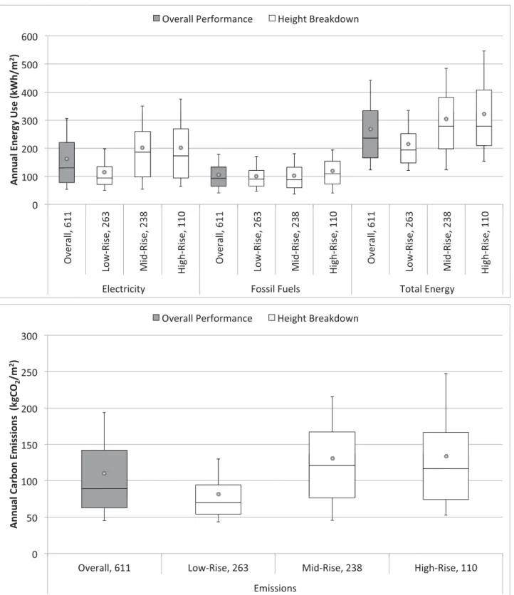
The box and whisker plot diagrams summarize the per-formance for the overall sample.Figure 2shows the dis-tribution of energy use intensity (kWh/m2) split between electricity and fossil fuels, as well as total consumption (top) and the corresponding total emissions (kgCO2/
m2) (bottom). In each graph, the median and interquar-tile range can be read from the box. The whiskers rep-resent the 10th and 90th percentiles, and the floating point is the mean. The median and first quartiles are sometimes used to define ‘typical’ and ‘good practice’ benchmarks respectively (DETR, 1998). For each vari-able, the overall performance is presented alongside the low/mid/high-rise split. The sample size for each result is provided on the x-axis label after the comma. The underlying data are also provided inTable 2.
The graphs inFigure 2reveal increasing energy con-sumption and emissions with height. Comparing the low- and high-rise categories, mean and median electri-city use increase by 76% and 85% respectively, while smaller rises are observed for fossil fuel (19% mean and 21% median). Gas represents approximately 95% of the total fossil fuel use in the sample. Consequently, its lower carbon intensity compared with mains electri-city means that the emissions trend follows the electrical result: 67% and 63% increases in mean and median annual emissions respectively. In addition to increases in the typical performance, the emissions interquartile range rises by a factor of 2.3 between low- and high-rise buildings showing that it is likely to be much more difficult to achieve low-energy tall buildings compared with low-rise.
Significant differences are found with height for energy consumption (electricity, fossil fuel and total) and emissions (ANOVA, p< 0.05). Interestingly, how-ever, the trends for energy use and height differ between electricity and fossil fuels. The Tukey HSD tests suggest that for electricity use the significant step is from low- to mid-rise buildings (low-to-mid and low-to-highp< 0.05; mid-to-highp> 0.05), whereas for fossil fuels the signifi -cant increase is from low- to high-rise (low-to-high and mid-to-highp< 0.05; low-to-mid p> 0.05). This diff er-ence may reflect the underlying relationships between
Table 1.Summary of data collected for this study.
Energy Other data Further data collection
BBP DEC EC Emporis
Skyscraper
Center e-PIMS 3DStock
Desktop survey Number of buildings in thefinal database with data from each source
Overall (out of 708) 217 341 192 213 13 277 708 660 (glazing 84)
Excluding predominantly electrically heated buildings (out of 611)
175 311 142 175 8 270 611 572 (glazing 72)
Building location
Address × × × × × × × ×
Latitude and longitude × × × ×
Energy consumption data
Annual energy-use data (kWh) × × × (some, but not
used)
Main heating fuel type ×
Building design
Floor area (m2) × (NLA/GIA) × (GIA) × (GIA) (limited, not used) (limited, not used) (yes, not used) (not used)
Internal use × (main
use)
× (list of uses)
× (main and side uses)
× (main and side uses)
× (main use) × (main use) × (detailed breakdown)
Height (storeys) × (very limited) × (detailed) × (detailed) × (very limited) × (detailed) × (estimated)
External surface to volume ratio (/m) ×
Glazing ratio (%) × (average
ratio)
Systems
Heating ventilation and air-conditioning × (limited) × × (limited, not used) (limited, not used) (limited, not used)
Dates
Construction × × × × (limited)
Demolition × × × (limited)
Note: BBP = Better Buildings Partnership database; DEC = Display Energy Certificate scheme; EC = Energy Challenge database; NLA = Net Lettable Area; GIA = Gross Internal Area.
6 D. GODO Y-SHIMIZ U ET A L.
energy demand, built form and the local climate. Energy end-use breakdown information is not available for the sample. However, all else being equal, height affects fossil fuel heating demand directly through changes in air temperature and wind speed, and via mechanisms such as the stack effect. Electricity use meanwhile varies
with access to daylight and solar gains, which are affected by the height of a building relative to the surrounding buildings. A recent study of high-rise buildings found a similar result, revealing that the change in daylight avail-ability with height depends on factors such as orientation and the neighbouring buildings (Li & Tsang,2008). Figure 2.Electricity, fossil fuel and total energy use (top) and emissions (bottom) for the overall sample.
Within the database, energy-use data come from the DEC, BBP and ECfiles. DECs predominantly cover public buildings, which may possibly have different typical pat-terns of use, internal gains and installed systems compared with the BBP and EC offices. Furthermore, previous work has shown that DEC offices typically have lower energy use than the BBP offices. Depending on the office type, the corresponding increase in median emissions between the DEC and BBP offices can be over 50% (Armitage et al., 2015). Therefore, if the buildings covered by the three sources have different typical built forms, it is theoretically possible that the observed energy–height trends simply reflect the underlying sources of data. Figure 3 presents the overall performance when the BBP, DEC and EC energy data are considered separately.3
As expected, the results reveal differences in typical energy use between the sources. While fossil fuel con-sumption is similar, electricity use is considerably higher for the BBP and EC offices compared with the DECs, resulting in mean emissions for the BBP sample being 40% higher than the DEC sample, while the EC mean is 17% higher still.
Despite the differences, however, the trend of increas-ing energy use from low- to high-rise buildincreas-ings can be observed for each source. For a few variables, a counter trend is observed, but these are small and statistically insignificant. For example, mean electricity use for the DECs decreases from mid- to high-rise buildings by approximately 5% (p> 0.05), whereas the corresponding increase from low-rise is significant (low-to-mid and low-to-highp< 0.05). Across the sources and variables, only mean fossil fuel consumption for the EC data is found to show no statistically significant difference with height (ANOVA,p> 0.05). This result shows that the overall trend of increasing energy use with height cannot be explained simply by systematic differences associated with the three original data sources.
In order to visualize the energy–height relationship in further detail,Figure 4shows the overall results, with the high-rise offices further subdivided. The tallest groups have very small sample sizes. Consequently, ANOVA tests were not carried out, and these results should be treated with some caution. However, the general trend of increasing energy use and emissions with height remains. Comparing the extremes, mean electricity and fossil fuel uses in the tallest group are 136% and 41% greater than the lowest respectively, while mean emis-sions are more than doubled (a 117% increase).
Multivariate regression
As previously discussed, energy consumption in build-ings is driven by their design, systems and use.
Table 2. Summary of energy and emissions for overall sample. Annual elect ricity use (kWh /m 2 ) Annual foss il fu el use (kWh /m 2 ) Annual tota l energy use (kWh /m 2 ) An nual emiss ions (kgCO 2 /m 2 ) Overall Low-r ise Mid-r ise Hig h-rise Overall Low -rise Mid-r ise Hig h-rise Overall Low -rise Mid-r ise High-ri se Ove rall Low -rise Mid-rise High-ri se C ount 611 263 238 11 0 –– – – –– – – –– – – Me an 164 114 201 20 1 105 100 102 120 269 2 15 304 321 110 82 13 0 134 75 th p ercent ile 221 134 259 27 0 133 120 133 154 334 2 53 381 408 142 94 16 7 166 Me dian 130 94 186 17 4 93 90 88 109 236 1 93 279 279 89 70 12 1 117 25 th p ercent ile 78 70 98 9 4 64 64 60 73 166 1 48 198 210 63 54 7 6 74 8 D. GODOY-SHIMIZU ET AL.
Consequently, the observed energy–height trends will partly reflect underlying differences in the typical charac-teristics of low-, mid- and high-rise offices. Since thefinal database includes several relevant variables, multivariate
analysis was undertaken to examine the impact of these factors on the energy–height relationship.
Table 3summarizes the characteristics of the build-ings within the database, alongside the high-, mid- and Figure 3.Electricity, fossil fuel and total energy use (top) and emissions (bottom) using energy data from each source independently.
low-rise splits. Due to the mix of sources of underlying data, complete information is not available for all of the buildings. Therefore,Table 3details the coverage of each variable in parentheses. The energy performance breakdown associated with several of the key variables is presented for reference in Figures 5–8, along with
the variation with building height. It should be noted that while each of the variables listed is separate, they may not be truly independent choices for building designers. For example, it has been acknowledged that achieving effective natural ventilation is especially com-plex for high-rise buildings (Gonçalves & Bode, 2011; Figure 4.Electricity, fossil fuel and total energy use (top) and emissions (bottom) for the overall sample, with more detailed height breakdown.
Wood & Salib, 2013). Consequently, during the design process, the choice of HVAC may be partly influenced by building height.
The trends are generally unsurprising: compared with low-rise, taller buildings are more likely to have
air-conditioning and to be located in higher density urban areas. Also they are typically newer and have more glaz-ing. In terms of physical form, the mean external surface area-to-volume ratiodecreases with increasing tallness. Tall buildings, above the height of adjacent blocks, Table 3.Summary of building characteristics of the low-, mid- and high-rise buildings, as well as the overall sample.
Variable Units Overall Low-rise Mid-rise High-rise
Sample size Number of buildings 611 263 238 110
A,BBuilding form (external envelope area/total volume)
Mean Ext Surface to Vol Ratio /m 0.202 0.251 0.157 0.149
(70.7%) (80.2%) (72.7%) (43.6%)
Glazing (overall envelope glazed percentage)
Avg Glazing Proportion 0.44 0.30 0.42 0.59
(11.8%) (9.1%) (8.8%) (24.5%)
BHVAC (main installed HVAC system)
Air Conditioned Proportion of buildings 0.58 0.37 0.74 0.72
Mech Vent Proportion of buildings 0.10 0.12 0.09 0.06
Mixed Mode Proportion of buildings 0.07 0.08 0.05 0.06
Nat Vent Proportion of buildings 0.24 0.40 0.10 0.15
Not Air Con Proportion of buildings 0.02 0.03 0.02 0.00
(99.8%) (100%) (99.6%) (100%)
BConstruction date (date of completion)
Pre-1970 Proportion of buildings 0.30 0.28 0.31 0.32
1970s Proportion of buildings 0.19 0.23 0.14 0.20
1980s Proportion of buildings 0.12 0.15 0.10 0.10
1990s Proportion of buildings 0.19 0.29 0.15 0.10
Post-1999 Proportion of buildings 0.19 0.05 0.30 0.28
(54.7%) (54.0%) (42.9%) (81.8%)
A,BRateable value (business taxation rate; correlates strongly with the data sources and may give an indication of building‘prestige’)
Avg Rateable Value £/m2 192 187 223 122
(92.0%) (98.9%) (93.7%) (71.8%)
A,BLocal urban area (rural urban classification, a description of the building local postcode, which may give an indication of the urban density of the area surrounding
each building)
Urban major conurbation (A1) Proportion of buildings 0.69 0.48 0.87 0.84 Urban minor conurbation (B1) Proportion of buildings 0.03 0.05 0.02 0.01
Urban city and town (C1) Proportion of buildings 0.27 0.46 0.12 0.15
Urban city and town in a sparse setting (C2) Proportion of buildings 0.00 0.00 0.00 0.00
Rural town and fringe (D1) Proportion of buildings 0.00 0.00 0.00 0.00
Rural town and fringe in a sparse setting (D2) Proportion of buildings 0.00 0.00 0.00 0.00 Rural village and dispersed (E1) Proportion of buildings 0.00 0.01 0.00 0.00 Rural village and dispersed in a sparse setting (E2) Proportion of buildings 0.00 0.00 0.00 0.00
(100%) (100%) (100%) (100%)
Note: The proportion of the sample for which each variable is known is provided in parentheses.A= variables included in analysis A (full coverage);B= variables included in analysis B (detail).
might be expected to have less party wall area than short ones. However, the result means that, in general, rather than being thinner and having less party wall area, taller buildings are more compact than shorter ones. A recent study of a small sample of buildings in Hong Kong found a similar trend, with mean ratios for 1–10, 11–20 and 20 + storey buildings of 0.20, 0.16 and 0.12/m respectively (Lam et al.,2004).
Due to the large differences in coverage between the variables, the multivariate regression using stepwise selection was carried out at two scales, summarized
below. In both cases, the analysis was repeated for elec-tricity use, fossil fuel use and emissions.
. Analysis A (full coverage): carried out using solely those variables that can currently be collected at a dis-aggregate level for England and Wales from the 3DStock model. The analysis included the three vari-ables labelled with ‘A’ inTable 3, as well as ‘height’. The sample size was 432 offices.
. Analysis B (detail): carried out using more detailed building information. The five variables in Table 3 Figure 5. Electricity, fossil fuel and total energy use (left) and emissions (right) for the sample, split by construction date.
Figure 6.Electricity, fossil fuel and total energy use (left) and emissions (right) for the sample, split by heating, ventilation and air-conditioning (HVAC) type.
Figure 7.Electricity, fossil fuel and total energy use (left) and emissions (right) for the sample, split by external surface-to-volume ratio.
labelled with‘B’were included along with height, cov-ering 215 offices. Glazing ratio was excluded from this analysis due to the low coverage.
Tables 4and5present the results of the GLM for elec-tricity use, fossil fuel use and emissions for analyses A and B respectively. The variables listed are those selected from the stepwise regression as optimizing the models. As pre-viously explained, a log-link function was used. Therefore, the impact of each variable can be estimated usingμ= exp (xβ) (Barber & Thompson,2004). For example, for analy-sis A, each additional storey is associated with a 2.2% rise in electricity use and a 2.4% rise in fossil fuels (calculated from Table 4 as exp(0.0216) = 1.022 and exp(0.0233) = 1.024 respectively). Figure 9 shows the actual and pre-dicted performance for electricity (top), fossil fuel (mid) and emissions (bottom) for analyses A (left) and B (right). The results show that the available data can provide a reasonable predictor of electricity use intensity in offices. In contrast, the variables explain very little of the variation in fossil fuel consumption, even under the more detailed analysis. The coefficients of determination (r2) for electri-city and fossil fuel are 0.21 and 0.02 for the‘full coverage’ models, but improve to 0.45 and 0.05 with the variables included in the ‘detail’ models, as shown in Figure 9. The emissions models follow electricity, reflecting the relative carbon intensities of the fuels, withr2-values of 0.21 and 0.45 respectively. Interestingly, the results are in stark contrast to thefindings of comparable analyses carried out recently for the London residential sector (Hamilton et al.,2017). Analyzing some of the same vari-ables, the study found no relationship of electricity con-sumption with height, but a strong relationship for gas, highlighting the differences in energy use between the domestic and non-domestic sectors in Britain.
Reassuringly, the overlapping variables have similar estimates between the two scales of analysis. For example, a £1/m2 increase in average rateable value (ARV) is associated with a 0.1% and 0.2% rise in
electricity consumption for the‘full coverage’and‘detail’ models respectively.4While the observed impact appears small, the interquartile range within the sample is £180/ m2, corresponding to a 32% rise in electricity use from the‘detail’ model. More detailed information about the relationship between rateable value and typical building characteristics is required to understand the drivers of the observed energy trends, but the variable may be a proxy for a qualitative building ‘prestige’ factor. This may be linked with variables such as air-conditioning, construction materials, glazing level, as well as internal use factors such as the presence of a gym or the intensity of use.
The results reveal a strong correlation between HVAC type and electricity use. Natural ventilation, for example, is associated with a 41% reduction in electricity use com-pared with air-conditioning, while mechanical venti-lation is between these extremes (26% reduction). It is interesting to note that, despite a difference in fossil fuel use shown inFigure 6(6.3% reduction in mean con-sumption between air-conditioned and naturally venti-lated buildings), HVAC type was excluded during the stepwise process from thefinal fossil fuel consumption model. This suggests that the net impact of HVAC type is predominantly on cooling and ventilation, rather than on heating. A similar trend can be found in DETR (1998). The benchmarks suggest a 166% rise in typical electricity use between naturally ventilated‘type 2’ and air-conditioned ‘type 3’ offices (with 40% attributable to cooling, fans and pumps), compared with only an 18% increase in typical fossil fuel use.5
The models suggest no clear relationship between energy consumption and location (urban/rural) as measured by the particular metric used (rural urban classification– RUC). This classification is included in the‘full coverage’electricity and emissions models. How-ever, the estimates show no simple trend, and the vari-able is excluded from the ‘detail’ models. It is worth noting, however, that RUC is a fairly crude descriptor Figure 8.Electricity, fossil fuel and total energy use (left) and emissions (right) for the sample, split by average rateable value.
Table 4.Results of analysis A (full coverage) generalized linear model, using a log-link function.
Parameter
Electricity-use model Fossil fuel-use model Emissions model
Estimated SE |t| Pr >|t| Estimated SE |t| Pr >|t| Estimated SE |t| Pr >|t| Intercept 5.2007 0.1731 30.045 < 2e–16 4.5433 0.0643 70.626 < 2e–16 4.7399 0.1483 31.954 < 2e–16
Height (storeys) 0.0216 0.0103 2.097 0.0365 0.0233 0.0083 2.799 0.0054 0.0237 0.0088 2.685 0.0075
Ext Surface to Vol Ratio (/m) –2.068 0.510 –4.053 0.0001 –1.542 0.437 –3.527 0.0005
Avg Rateable Value (£/m2) 0.0009 0.0003 3.409 0.0007
–0.0003 0.0002 –1.416 0.1575 0.0007 0.0002 2.869 0.0043 RUC Type A1 0 0 RUC Type B1 –0.319 0.193 –1.652 0.0992 –0.258 0.166 –1.559 0.1198 RUC Type C1 –0.263 0.084 –3.145 0.0018 –0.210 0.072 –2.928 0.0036 RUC Type D1 0.770 0.667 1.155 0.2490 0.657 0.571 1.15 0.2508 RUC Type E1 –0.305 0.670 –0.455 0.6492 –0.429 0.574 –0.747 0.4556 AIC 5036 4657.6 4605.3 Pseudo-r2 0.2629 0.0219 0.2524
Note: AIC = Akaike Information Criterion.
Table 5.Results of Analysis B (Detail) generalized linear model, using a log-link function.
Parameter
Electricity-use model Fossil fuel-use model Emissions model
Estimated SE |t| Pr >|t| Estimated SE |t| Pr >|t| Estimated SE |t| Pr >|t|
(Intercept) –4.232 3.053 –1.386 0.1671 4.430 0.079 56.391 < 2e–16 –1.133 2.704 –0.419 0.6756
Height (storeys) 0.0237 0.0089 2.666 0.0083 0.0290 0.0095 3.056 0.0025 0.0247 0.0079 3.132 0.0020
HVAC type AC 0 0
HVAC type MM –0.033 0.116 –0.287 0.7741 –0.030 0.102 –0.29 0.7717
HVAC type MV –0.306 0.099 –3.081 0.0023 –0.208 0.088 –2.368 0.0188
HVAC type NV –0.520 0.092 –5.667 4.8e–8 –0.373 0.081 –4.592 7.6e–6
Ext Surface to Vol Ratio (/m) –1.635 0.565 –2.896 0.0042 –1.582 0.500 –3.165 0.0018
Construction date (year) 0.0047 0.0015 3.096 0.0022 0.0029 0.0013 2.194 0.0294
Avg Rateable Value (£/m2) 0.0016 0.0004 4.06 0.0001 0.0011 0.0003 3.324 0.0011
AIC 2367.3 2297.9 2169.2
Psuedo-r2 0.5704 0.0571 0.5380
Note: AIC = Akaike Information Criterion.
14 D. GODO Y-SHIMIZU E T A L.
of urban character and location, and that the postcode area (at which RUC is measured) varies significantly. Consequently, it may not provide a useful indication of the surroundings of each building, for energy perform-ance purposes. Alternative aggregate geographic data are available for the UK, including land use and popu-lation data. However, these are still broad proxies for urban form, and provided at varying levels of aggrega-tion. It may be better to explore the relationship between urban form and energy use further using more detailed quantitative metrics. 3DStock provides a detailed
description of built form at a disaggregate scale. There-fore, work is currently ongoing to integrate calculations that describe the physical surroundings for each building in detail.
Regulations covering the conservation of fuel and power were introduced for new non-domestic buildings in the UK in 1974 and have grown progressively more stringent over time, setting minimum requirements for building envelope and plant characteristics, as well as standardized methods for estimating energy consump-tion (King,2007). Furthermore, while modern buildings Figure 9.Actual and predicted electricity use (top), fossil fuel use (middle) and emissions (bottom) based on analysis A, full coverage (left) and B, detail, (right).
may have better insulation and infiltration standards than older ones at the point of construction, fabric and plant efficiency may also deteriorate over time. There-fore, it is interesting that no correlation was found between construction date and fossil fuel use.
The results suggest that newer buildings are associated with higher electricity use. A possible explanation for this electricity trend may be that modern buildings are used more intensively than older ones, through higher occu-pancy density and information technology (IT) use. It should be noted, however, that more intensive use typi-cally results in higher internal gains, which may be expected to offset some of the demand for space heating: but this is not reflected in the fossil fuel use. Overall, the model suggests that between offices constructed in 1974 and 2010, there is an 18.4% increase in electricity use inten-sity. The fact that the buildings designed to meet the tough-est regulations have the hightough-est emissions highlights the difficulty in improving the building stock as a whole.
The external surface-to-volume ratio provides a description of a building’s overall compactness, account-ing for party boundaries and buildaccount-ing size. Theoretically, the variable is related to the potential for heat transfer, solar gains, daylight, natural ventilation and infiltration, which all occur at the external envelope. In this light, it is interesting to note that neither modelfinds a significant relationship with fossil fuel use. A possible explanation for the lack of any clear trend may be glazing ratio, which drops from a mean of 60% to 21% from the most to least compact buildings. Within the database, only 45 buildings include data on both glazing and exter-nal surface-to-volume ratio, therefore this subsample is tiny. However, similar positive relationships between average glazing and compactness have been observed in two studies of high-rise buildings in Hong Kong (Lam et al., 2004; Li & Tsang,2008), as well as the US (Winiarski, Halverson, & Jiang, 2008). In the former, for example, the mean glazing ratios for the most and least compact quartile of buildings were 47% and 30% respectively. If it is true that building compactness corre-lates negatively with glazing, then the corresponding effect on building U-values may explain the trend. Sig-nificantly, Steemers (2003) suggests that in order to minimize energy consumption, glazing ratios should decrease with height, while Raji, Tenpierik, and van den Dobbelsteen (2016) suggest that window-to-wall glazing ratios should be between 30% and 50% depend-ing on the thermal performance of the envelope. External surface-to-volume ratio is found in the present work to be associated with a drop in electricity use: from the
‘detail’ model, an increase of 0.1/m corresponds to an 18% drop in electricity consumption. This suggests that the increased access to daylight and opportunity for
natural ventilation may offset the corresponding added exposure to solar gains.
Across both scales of analysis, the results show that height is a significant predictor of energy use, even accounting for other variables. This means that the energy/height trends observed inFigure 2are not simply a reflection of the fact that low-, mid- and high-rise buildings have different characteristics (Table 3). From the ‘detail’ model, one additional storey is associated with a 2.4% increase in electricity use and a 2.9% increase in fossil fuel use. The corresponding impact on carbon emissions is a rise of 2.5%. Based on the mean perform-ance of the sample, this indicates that changing from low- to high-rise (from five to 15 storeys) results in increases in mean electricity and fossil fuel consumption of 44 and 33 kWh/m2respectively.
Building height influences energy consumption directly through mechanisms such as changes in external temperature and wind speed with altitude, access to day-light and solar gains, as well as the need for lifts (eleva-tors). However, the net impact on any specific building will depend on factors such as occupancy behaviour, building design and the internal systems. For example, reductions in artificial lighting will only be achieved if the controls are connected to daylight sensors. However, this may not be the case: a survey of an office in the US found poor daylight controls in reality due to issues such as interior layouts (Day, Theodorson, & Van Den Wymelenberg,2012), while a survey of 15 offices in the UK found very poor integration between the solar and daylighting controls (Cunill, Serra, & Wilson, 2007). Examination of energy end-uses in conjunction with building modelling will be required to determine the underlying drivers for the observed trends. However, the fact that height correlates positively with both electri-city and fossil fuel use suggests that any reduction in artificial lighting demand in taller buildings due to greater access to daylight is overwhelmed by other fac-tors, such as the need to deal with increased solar gains.
Conclusions and further work
This paper presents the results of an examination of the performance of a sample of 611 offices in England and Wales. Disaggregate energy data from the DEC, BBP and EC databases were used in conjunction with other building data as well as the results of a survey undertaken by the authors. Statistical tests were carried out to explore the drivers of energy consumption, with a focus on understanding the impact of building height.
Considering the overall change in performance with height, it was found that mean electricity and fossil fuel use increase by 77% and 20% respectively between
and high-rise offices (defined as ≤ 5 and > 10 storeys respectively), with a corresponding rise in mean CO2
emissions of 67%. The variation in 10th percentile emis-sions with height is small, suggesting that achieving low-carbon performance in tall buildings is possible. How-ever, a near doubling of 75th percentile emissions indi-cates that this is rarely achieved. Within the sample, the low-, mid- and high-rise offices have different typical characteristics. Therefore, GLM was used to examine the underlying drivers of the observed energy–height trends. Height is shown to be a significant predictor of energy, even accounting for variables such as HVAC type and date of construction. Each storey is associated with 2.4% and 2.9% increases in mean electricity and fossil fuel use respectively, corresponding to a 31% increase in emissions between low- and high-rise buildings.
The direct effects of height on energy consumption are a result of the interaction between a building and its local environment. For example, all other things being equal, an increase in height will raise the amount of daylight and solar gains entering a building, poten-tially reducing the demand for artificial light in its per-imeter zones, but increasing the risk of overheating. Data on the energy end-use breakdown are not available for this study. However, the results suggest that the benefits associated with height, such as a reduced need for artificial lighting, may be outstripped by factors that increase electricity and fossil fuel use, such as an increased demand for cooling or mechanical ventilation associated with solar gains.
This paper is part of an ongoing study examining the relationship between energy consumption and height within the UK building stock. The study will continue, focusing on two areas of interest:
. Thermal modelling
Statistical studies of the kind presented here cannot determine causality. Work is currently ongoing to use building modelling to examine the mechanisms that drive the observed trends. In particular, this will help to quantify the theoretical relative impact of height, envelope and surrounding buildings on the demand for electricity and fossil fuel.
. Character of the urban area
Solar gains and daylight will vary with the relative height of a building compared with its surroundings, rather than its absolute height. However, the existing publicly available urban form data were found to be insufficiently detailed for use as an indicator of build-ing energy use. Therefore, work is ongobuild-ing to inte-grate detailed and quantitative descriptors of urban form into 3DStock to better describe the relationship between each building and its local area.
The analysis presented in this paper shows that increases in building height are associated with higher electricity and fossil fuel consumption in offices. The dri-vers for the observed trends are not clear cut. However, the available data suggest that they cannot simply be explained by factors such as the presence of air-con-ditioning. It has previously been suggested that it is
‘undoubtedly true’ that tall buildings were, by their nature, more energy intensive than shorter ones (Can-gelli & Fais,2012, p. 40). While low-emission, high-rise buildings exist within the sample, the analysis suggests that they are still the exceptions to the rule.
Notes
1. The character of vertical transportation is also linked to building height. However, a study of energy end-use in high-rise offices in Hong Kong found that this accounts for only 3.2% of total energy use (Lam et al.,2004), in line with similarfigures for the UK (DETR,1998). 2. This result is not actually reported but can be inferred
from data included in the paper.
3. The total sample sizes appear to be larger than the pre-vious graph because some buildings appear in multiple data sets.
4. Rateable value is calculated by the UK government for the purposes of assessing property taxes or‘rates’. 5. The office types defined by DETR (1998) include a
pack-age of characteristics, not just HVAC type, so the com-parison should be treated with caution. However, data are provided on the energy end-use breakdown.
Acknowledgements
Special thanks are due to Chris Botten and Better Buildings Partnership. The authors also thank Sung-Min Hong, Rob Lid-diard, Paul Ruyssevelt and the London Mayor’s Energy Chal-lenge for the supply of data.
Disclosure statement
No potential conflict of interest was reported by the authors.
Funding
This work was supported by the Engineering and Physical Sciences Research Council (EPSRC)-funded‘High-Rise Build-ings: Energy and Density’[grant number EP/N004671/1] and the EPSRC-funded‘RCUK Centre for Energy Epidemiology’ [grant number EP/K011839/1].
ORCID
Ian Hamilton http://orcid.org/0000-0003-2582-2361 Michael Donn http://orcid.org/0000-0002-4716-4286 Stephen Evans http://orcid.org/0000-0002-6692-907X
References
Ali, M. M., & Moon, K. S. (2007). Structural developments in tall buildings: Current trends and future prospects.
Architectural Science Review,50(3), 205–223.
Armitage, P., Godoy-Shimizu, D., Steemers, K., & Chenvidyakarn, T. (2015). Using Display Energy Certificates to quantify public sector office energy consump-tion.Building Research & Information,43(6), 691–709. Baker, N. V., & Steemers, K. (1994).The LT Method 2.0: An
energy design tool for non-domestic buildings. Cambridge: Cambridge Architectural Research Limited and the Martin Centre for Architectural and Urban Studies.
Barber, J., & Thompson, S. (2004). Multiple regression of cost data: Use of generalised linear models. Journal of Health Services Research & Policy,9(4), 197–204.
Cangelli, E., & Fais, L. (2012). Energy and environmental per-formance of tall buildings: State of the art. Advances in Building Energy Research,6(1), 36–60.
Chartered Institute of Building Services Engineers (CIBSE). (2006).Guide A: Environmental design. London: Author. Chau, C. K., Hui, W. K., Ng, W. Y., & Powell, G. (2012).
Assessment of CO2 emissions reduction in high-rise
con-crete office buildings using different material use options.
Resources, Conservation and Recycling,61, 22–34.
Cunill, E., Serra, R., & Wilson, M. (2007, November).Using daylighting controls in offices? Post occupancy study about their integration with the electric lighting. Proceedings of PLEA2007 – The 24th Conference on Passive and Low Energy Architecture, Singapore.
Day, J., Theodorson, J., & Van Den Wymelenberg, K. (2012). Understanding controls, behaviors and satisfaction in the daylit perimeter office: A daylight design case study.
Journal of Interior Design,37(1), 17–34.
Department for Business, Energy & Industrial Strategy (BEIS). (2016).Building energy efficiency survey: Office sector, 2014– 15. London: Author.
Department of Energy & Climate Change (DECC). (2013).
Exploring the use of Display Energy Certificates. London: Author.
Department of the Environment, Transport and the Regions (DETR). (1998).Energy consumption guide 19: Energy use in offices. London: DETR.
Ellis, P. G., & Torcellini, P. A. (2005, August).Simulating tall buildings using EnergyPlus. Proceedings of IBPSA International Conference, Montreal, Canada.
Emmerich, S. J., & Persily, A. K. (1998). Energy impacts of infiltration and ventilation in US office buildings using multi-zone airflow simulation. Proceedings of ASHRAE IAQ and Energy 98 conference. New Orleans, LA, USA. Evans, S., Liddiard, R., & Steadman, P. (2017). 3DStock: A new
kind of three-dimensional model of the building stock of England and Wales, for use in energy analysis.
Environment and Planning B: Urban Analytics and City Science,44(2), 227–255.
Foraboschi, P., Mercanzin, M., & Trabucco, D. (2014). Sustainable structural design of tall buildings based on embodied energy.Energy and Buildings,68, 254–269. Godoy-Shimizu, D., Armitage, P., Steemers, K., &
Chenvidyakarn, T. (2011). Using Display Energy Certificates to quantify schools’ energy consumption.
Building Research and Information,39(6), 535–552.
Gonçalves, J., & Bode, K. (2011). The importance of real life data to support environmental claims for tall buildings.
CTBUH Journal, (2), 24–29.
Hamilton, I., Evans, S., Steadman, P., Godoy-Shimizu, D., Donn, M., Shayesteh, H., & Moreno, G. (2017). All the way to the top! The energy implications of building tall cities.Energy Procedia,122, 493–498.
Hamilton, I. G., Summerfield, A. J., Lowe, R., Ruyssevelt, P., Elwell, C. A., & Oreszczyn, T. (2013). Energy epidemiology: A new approach to end-use energy demand research.
Building Research and Information,41(4), 482–497. Hemsath, T. L., & Bandhosseini, K. A. (2015). Sensitivity
analysis evaluating basic building geometry’s effect on energy use.Renewable Energy,76, 526–538.
Hong, S. M., Paterson, G., Mumovic, D., & Steadman, P. (2014). Improved benchmarking comparability for energy consumption in schools. Building Research and Information,42(1), 47–61.
Hong, S., & Steadman, P. (2013).An analysis of Display Energy Certificate for public buildings, 2008 to 2012. London: UCL Energy Institute.
Jones, P., Patterson, J., & Lannon, S. (2007). Modelling the built environment at an urban scale—Energy and health impacts in relation to housing. Landscape and Urban Planning,83(1), 39–49.
King, T. (2007, November).The history of the building regu-lations and where we are now. Paper presented at HBF Technical Conference: The road to zero carbon is paved with Building Regulations. London, UK.
Lam, J. C., Chan, R. Y., Tsang, C. L., & Li, D. H. (2004). Electricity use characteristics of purpose-built office build-ings in subtropical climates. Energy Conversion and Management,45(6), 829–844.
Li, D. H., & Tsang, E. K. (2008). An analysis of daylighting per-formance for office buildings in Hong Kong.Building and Environment,43(9), 1446–1458.
Oldfield, P., Trabucco, D., & Wood, A. (2009). Five energy generations of tall buildings: An historical analysis of energy consumption in high-rise buildings.Journal of Architecture,
14(5), 591–613.
Parasonis, J., Keizikas, A., & Kalibatiene, D. (2012). The relationship between the shape of a building and its energy performance. Architectural Engineering and Design Management,8(4), 246–256.
R Development Core Team. (2008). R: A language and environment for statistical computing. Vienna, Austria: R Foundation for Statistical Computing. Retrieved from
http://www.R-project.org
Raji, B., Tenpierik, M. J., & van den Dobbelsteen, A. (2016). An assessment of energy-saving solutions for the envelope design of high-rise buildings in temperate climates: A case study in the Netherlands. Energy and Buildings, 124, 210–221.
Ramesh, T., Prakash, R., & Shukla, K. K. (2010). Life cycle energy analysis of buildings: An overview. Energy and Buildings,42(10), 1592–1600.
Ratti, C., Baker, N., & Steemers, K. (2005). Energy consump-tion and urban texture. Energy and Buildings, 37(7), 762–776.
Resch, E., Bohne, R. A., Kvamsdal, T., & Lohne, J. (2016). Impact of urban density and building height on energy use in cities.Energy Procedia,96, 800–814.
Steadman, P. (2014). Density and built form: Integrating
‘spacemate’ with the work of Martin and March.
Environment and Planning B: Planning and Design,41(2), 341–358.
Steemers, K. (2003). Energy and the city: Density, buildings and transport.Energy and Buildings,35(1), 3–14.
Tamošaitienė, J., & Gaudutis, E. (2013). Complex assessment of structural systems used for high-rise buildings. Journal of Civil Engineering and Management,19(2), 305–317. Tian, W., & Choudhary, R. (2012). A probabilistic energy
model for non-domestic building sectors applied to analysis of school buildings in greater London.Energy and Buildings,
54, 1–11.
Treloar, G. J., Fay, R., Ilozor, B., & Love, P. E. D. (2001). An analysis of the embodied energy of office buildings by height.Facilities,19(5/6), 204–214.
Winiarski, D. W., Halverson, M. A., & Jiang, W. (2008, August). DOE’s commercial building
benchmarks-development of typical construction practices for building envelope and mechanical systems from the 2003 CBECS.
Proceedings of 2008 ACEEE Summer Study on Energy Efficiency in Buildings, California, USA.
Wong, N. H., Jusuf, S. K., Syafii, N. I., Chen, Y., Hajadi, N., Sathyanarayanan, H., & Manickavasagam, Y. V. (2011). Evaluation of the impact of the surrounding urban mor-phology on building energy consumption.Solar Energy,85
(1), 57–71.
Wood, A., & Salib, R. (2013).Guide to natural ventilation in high rise office buildings. Chicago: Routledge.
Wright, A. (2008). What is the relationship between built form and energy use in dwellings?Energy Policy,36(12), 4544–4547. Yalcintas, M., & Aytun Ozturk, U. (2007). An energy bench-marking model based on artificial neural network method utilizing US commercial buildings energy consumption sur-vey (CBECS) database. International Journal of Energy Research,31(4), 412–421.