Algorithms for Cable Network Design on Large-scale Wind Farms

1. INTRODUCTION

Algorithms for Cable Network Design on

Large-scale Wind Farms

Constantin Berzan Tufts University Kalyan Veeramachaneni

James McDermott Una-May O’Reilly

Evolutionary Design and Optimization Group Computer Science and Artificial Intelligence Laboratory

Massachusetts Institute of Technology

Abstract. _{Laying out the network of power cables between wind}

tur-bines and substations incurs a significant cost when building a wind farm. For small farms, an expert can often identify a good layout by hand, or by simulating all the possible layouts. But for larger farms, these ap-proaches are no longer applicable. We present some initial work towards automating the design of cabling layouts for large-scale wind farms. We build a problem model that incorporates the relevant real-world con-straints, and then decompose the problem into three layers: the circuit, the substation, and the full farm. In the case when there is a single cable type, the circuit and substation layers map to graph problems (the un-capacitated and un-capacitated minimum spanning tree). For the full farm layer, we present a greedy top-down algorithm to find a feasible solu-tion. In the case when there are multiple cable types, we focus on the first layer, presenting an algorithm to find the optimal circuit. We then discuss under what conditions the problem can be simplified to the case with a single cable type.

1

Introduction

A collector system is the network of cables and transformers that harvest the energy from wind turbines and make it available to the electric grid. Designing the collector system for a wind farm is a complex problem, and a good design can lead to lower construction and operation costs.

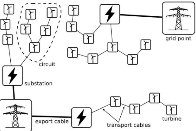
To define the problem, we consider six types of entities. The turbines pro-duce energy from wind. The energy needs to be delivered to nearbygrid points. Turbines cannot be connected directly to the grid. Instead, sets of turbines are connected to substations, using transport cables. The turbines connected to a substation form a tree topology, and each branch rooted at the substation is called acircuit. Each segment of cable in a circuit needs to have enough capac-ity for the number of turbines downstream. Finally, each substation is connected

to a grid point with a single high-voltageexport cable. Figure 1 shows an exam-ple layout. There are multiexam-ple types of transport cables, with different costs and capacities. There is also a limit on how many turbines can be connected to the same substation. The cost of a substation depends on the location where it is built. Similarly, the cost of a transport cable depends on the terrain in which it is buried. grid point substation turbine transport cables export cable circuit

Fig. 1: An example layout with two grid points, three substations, and a total of 20 turbines in five circuits.

The collector system design problem is to place the substations, and deter-mine the network of cables, such that all turbines are connected via substations to the grid, all capacity constraints are satisfied, and the total cost is minimized. For small farms, this problem is typically solved by hand, or by using brute-force techniques that try all possible cable layouts. This quickly becomes infeasible for larger farms, and cleverer approaches have started to appear in the literature [3]. We are interested in developing an automated technique for designing the collec-tor system of large farms (up to 1000 turbines). This paper presents some initial steps in that direction.

The rest of this paper is structured as follows: In section 2, we present our model of the problem. In section 3 we propose a decomposition into three layers: the Circuit, Substation, and Full Farm Problem. In section 4 we discuss our ter-rain grid and cable cost function. In section 5 we investigate the case when there is a single cable type, because this makes the problem much simpler. We show that the Circuit and Substation problems map to well-studied graph problems, and we present a top-down greedy algorithm for finding a feasible solution to the Full Farm Problem. Next, we look at multiple cable types in section 6. We present an algorithm for finding the optimal solution to the Circuit problem. In section 7, we present some experiments to determine under what conditions the

2. OUR MODEL problem can be simplified to a single cable type. We conclude and discuss ideas for future work in section 8.

2

Our Model

We worked with a domain expert to extract a model of the problem that incorpo-rates all the relevant real-world constraints. We only consider a simplification of the problem, where the substation locations are known. We are thus concerned only with connecting turbines to substations. Furthermore, we assume that all turbines have the same power rating. This allows us to express all constraints in numbers of turbines, instead of amperes or megawatts. An instance of the problem contains the following input data:

– An arrayT of turbines described by their location:ti= (xi, yi).

– An arrayS of substations described by their location:si= (xi, yi).

– The maximum number of turbines per substation:nS. (This constraint comes

from the maximum power rating of a substation.)

– The maximum number of turbines per circuit: nC. (This constraint comes

from the “thickest” type of cable available.)

– The costKC(u, v, n) of connecting two sites with a transport cable of

capac-ityn. A site can be a turbine or a substation. The value ofnranges from 1 (a cable for a single turbine) tonC (a cable of the maximum allowed capacity).

A solution is an array of circuitsCij for each substationsi ∈S. Each circuit

is a tree, represented by a tuple (Vij, Eij).Vij={vijk}is a set of turbines, and

Eij ={eijk}is a set of cables between the turbines inVij. The turbinevij0that connects directly to the substation is called the circuit root. The cost of a circuit Cij = (Vij, Eij) attached to substationsi is given by:

K(Cij) =KC(vij0, si,|Vij|) +

X

(u,v)∈Eij

KC(u, v, fuv)

where fuv is the flow through the directed edge (u, v). Each turbine produces

one unit of flow:fuv= 1 +P₍t,u)∈Eijftu.

The cost of a substation is simply the added cost of its circuits. (The substa-tion locasubsta-tions are fixed, so we do not consider the cost of building the substasubsta-tions, or the cost of connecting them to the grid.) The total cost of a solution is:

Ktotal= X

si∈S

X

Cij∈si

K(Cij)

Our goal is to minimizeKtotalunder these constraints:

– Each turbine appears in exactly one circuit, i.e.Vij form a partition ofT.

– All circuits are trees, i.e.Eij is a tree ofVij for each circuit.

– No transport cable is overloaded, i.e.fuv ≤nC for all (u, v) in allEij.

– No substation is overloaded, i.e.P

3

Problem Decomposition

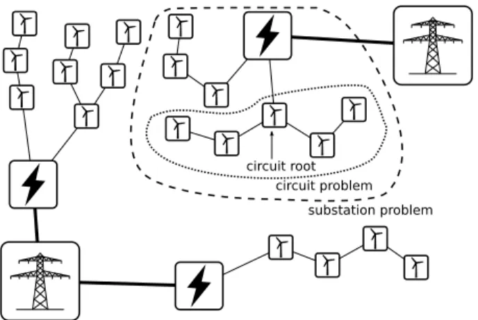
We find it useful to divide the full cabling problem into smaller subproblems, which can be investigated individually. Figure 2 illustrates the three layers that we consider.

circuit problem circuit root

substation problem

Fig. 2: The full farm problem, one substation problem, and one circuit problem.

The Circuit Problem1. This is the simplest and smallest version of the prob-lem. We are given a set of turbinestithat form a single circuit, andt0is the root

of the circuit (the turbine that connects directly to the substation). The goal is to connect all the turbines to the root in a way that minimizes cost. The solution is a spanning tree ofti. The cost of each edge is given byKC(u, v, n), wherenis

the number of turbines downstream. From discussions with our domain expert, a typical circuit contains at most 14 turbines (each rated at 1.5 MW).

The Substation Problem. This is a problem of intermediate complexity. We are given a substation s, and the set of turbinesti that connect to it. The goal

is to connect the turbines to the substation as inexpensively as possible. The solution looks like a spanning tree rooted at s. We do not know how many circuits to use, or which turbines to assign to which circuits. No circuit can have more than nC turbines. From discussions with our domain expert, a typical

substation contains at most 42 turbines (i.e. 3 circuits at maximum capacity). The Full Farm Problem. This is the cabling problem in its full complexity. We are given a set of substations, and a set of turbines. We do not know how

1

The name ‘circuit’ comes from the electrical circuit formed by a set of turbines. It is unrelated to the notion of circuit in graph theory.

4. THE CABLE COST FUNCTION to assign turbines to circuits, or circuits to substations. The solution looks like a forest of spanning trees rooted at the substations. The goal is to be able to solve the full problem for up to 1000 turbines.

4

The Cable Cost Function

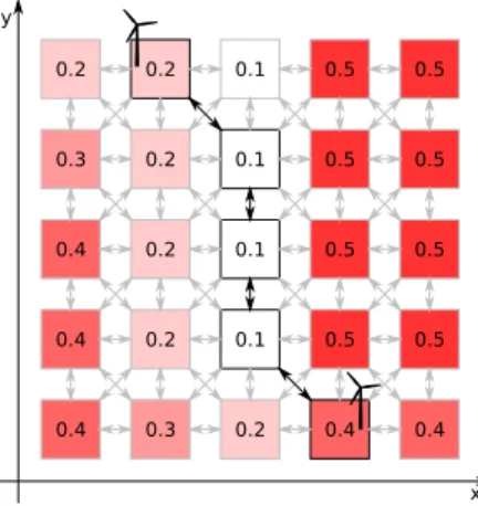
In the real world, the cost of a cable from one location to another depends on the type of cable used, and the terrain in which it is buried. We model the topography of the terrain using a 2D grid of cells. After we place our sites (turbines and substations) on this grid, we compute all pairwise costsbetween them. Each cell is square and has eight neighbors. To obtain the pairwise costs k(u, v), we run Dijkstra’s single-source shortest path algorithm starting at each site, and add up the cell values on the least-cost path between sites. Figure 3 shows an example. For a grid of V cells, each instance of Dijkstra’s algorithm runs inO(V logV), since the number of edges is roughly four times the number of nodes in the graph. The total running time is thus O(N ·V logV), whereN is the number of sites (turbines and substations).

0.2 0.2 0.1 0.5 0.5 0.3 0.4 0.4 0.4 0.2 0.1 0.5 0.5 0.2 0.1 0.5 0.5 0.2 0.1 0.5 0.5 0.3 0.2 0.4 0.4 x y

Fig. 3: An example terrain grid. The numbers in the cells indicate cost, and the arrows indicate cell connectivity. The shortest path between the two turbines indicated has cost 0.2 +√2·0.1 + 0.1 + 0.1 +√2·0.4. (We add up the cell values, including source and destination, and we multiply by√2 for diagonal steps.)

We then determine the cost functionKC(u, v, n) based on the pairwise cost

k(u, v), and the number n of turbines whose energy that cable transports. We present the single-cable-type and multiple-cable-types cases separately, because the problem is much simpler in the former case.

4.1 A Single Cable Type

With a single cable type, the cable cost does not depend on the amount of energy flow on the cable (i.e., thenparameter is ignored). The cost function thus differs from the pairwise cost by only a constant. Without loss of generality, we can assume that the constant is one:

KC(u, v, n) =k(u, v)

4.2 Multiple Cable Types

With multiple cable types, the pairwise cost between sites serves as a rough notion of distance, and the cost of a cable also depends on the amount of energy flow through it. Following a recent paper by Dutta and Overbye [3], we obtain information about cable costs from the publicly available documents of the Black Nubble wind farm [11] in Maine. This farm uses 3 MW turbines with a power rating of 52.3 A each. The cost of trenching is $15 per foot, and the cable types are as follows:

cable type rating (amps) capacity (# turbines) adjusted capacity cost ($/ft)

1/0 AWG 150 2.9 5.8 5

4/0 AWG 211 4.0 8.0 10

500 kcmil 332 6.3 12.6 12

750 kcmil 405 7.7 15.4 26

1000 kcmil 462 8.8 17.6 38

We divide the turbine power rating by two, and add the trenching cost, to obtain our final cost function:

KC(u, v, n) =        20·k(u, v) : n≤5 25·k(u, v) : n≤8 27·k(u, v) : n≤12 41·k(u, v) : n≤15

5

Solutions for a Single Cable Type

When there is a single cable type, our problems map nicely to existing problems in the literature. We first discuss these relationships, and then present an efficient algorithm for finding a feasible solution to the full farm problem.

5.1 Relationship to Existing Problems

MST for the Circuit Problem. A spanning tree of an undirected graph is a subgraph that connects all nodes, and contains no cycles. The Minimum Spanning Tree (MST) of an undirected graph is the spanning tree with minimum total edge cost, out of all spanning trees. There exist efficient algorithms for

5. SOLUTIONS FOR A SINGLE CABLE TYPE computing the MST of a graph. For example, Prim’s algorithm [14] runs in O(E+VlogV), where V is the number of vertices in the graph, and E is the number of edges. The MST of a set of turbines gives the optimal solution to the Circuit Problem.

CMST for the Substation Problem. The Capacitated Minimum Spanning Tree (CMST) Problem is a constrained version of the MST. Amberg, Domschke and Voß [1] provide a good survey. One node is designated as the root, and the capacity constraint states that no branch from the root can have more thanK nodes. The CMST is the shortest spanning tree that satisfies this capacity con-straint. This is an NP-hard problem [13]. There have been numerous exact and approximate algorithms proposed for solving it [1, 4, 16]. Any existing approach to solving the CMST applies directly to our problem. The CMST with the sub-station as the root, andnCas the capacity constraint gives the optimal solution

to the Substation Problem.

LAND for the Full Farm Problem. The Local Access Network Design (LAND) Problem is concerned with connecting end users to the backbone net-work. This is the second stage in a hierarchical design process, where the first stage determines the backbone itself [4]. LAND is typically split into subprob-lems, which are solved sequentially. For example, one decides how many con-centrators to use (concentrator quantity problem), where to place them (con-centrator location problem), how to assign terminals to con(con-centrators (terminal clustering problem), and how to connect the terminals to their concentrators (terminal layout problem) [10]. These four problems correspond roughly to: de-ciding how many substations to use, where to put them, how to assign turbines to substations, and how to connect the turbines to their respective substations. Solutions to the terminal clustering and layout problems apply directly to our Full Farm Problem. The concentrator quantity and location problems apply to an extension of our problem, where the substation locations are not known in advance.

5.2 Finding a feasible solution to the Full Farm Problem

Knowing that solutions to LAND carry over to our Full Farm Problem, we now present one such approach. Our algorithm proceeds in a greedy top-down manner that closely resembles a hierarchical solution to LAND, described by Gouveia and Lopes [10]. First, we associate turbines to substations, ensuring that the substation capacity nS is satisfied. Then, we arrange the turbines of

each substation into circuits, ensuring that the circuit capacity nC is satisfied.

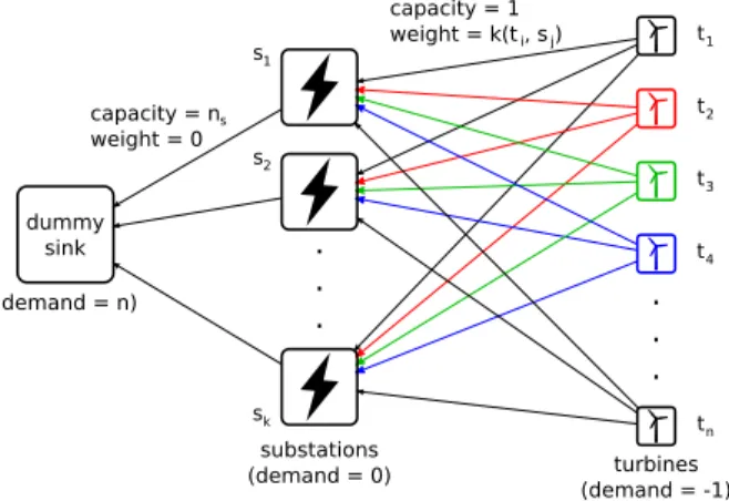
We formulate the problem of associating turbines to substations as a minimum-cost flow problem. Each turbine is a source producing one unit of flow, and each substation is a sink accepting at most nS units of flow. Figure 4 illustrates the

s as the pairwise cost fromt to s. Our goal is to assign all turbines to substa-tions in a way that minimizes cost, while satisfying capacity constraints. (We can visualize this as choosing the best out of all feasible forests of star trees rooted at substations.) To find this assignment, we run Goldberg’s2 _min-cost flow algorithm [5]. dummy sink . . . ._. . t1 t2 t3 t4 tn s1 s2 sk capacity = n weight = 0 s (demand = n) substations (demand = 0) turbines (demand = -1) capacity = 1 weight = k(t , s )i j

Fig. 4: Flow network for determining the association of turbines to substations.

Once we obtain a turbine-to-substation assignment, we are left with several substation problems to solve. For each of these problems, we approximate the CMST with the Esau-Williams (EW) heuristic, usingnC as the capacity limit.

Gavish [4] discusses how EW works, and Kershenbaum [9] shows how to imple-ment it inO(n2_logn).

5.3 Results and Discussion

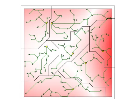
Figure 5 shows an example layout for 200 nodes with a uniform random dis-tribution. For the reader’s convenience, we have delimited the area spanned by the tree rooted at each substation. Notice that for substation 0, cables from two different circuits cross over each other.

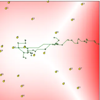
Figure 6 shows an example layout for 1000 nodes with a uniform random distribution. (Precomputing the pairwise costs took 23.6 seconds on a 200x200 terrain grid, and finding the actual solution took only 2.1 seconds3.) The layout looks quite messy, with cables criss-crossing everywhere. Notice that there are many substations in the center-left area, and very few in the center-right area. This forces the turbines in the center-right area to connect to far-away substa-tions. To illustrate this, Figure 7 shows the same layout, hiding every tree except the one rooted at substation 12.

2

The source code retrieved fromhttp://www.igsystems.com/cs2/download.html re-quires a license if used commercially.

3

5. SOLUTIONS FOR A SINGLE CABLE TYPE

Fig. 5: Example layout for 7 substations, 193 turbines, nS = 30, andnC = 10.

Yellow circles represent substations. Smaller green circles represent turbines. The background shows the terrain grid (white = cheap, red = expensive).

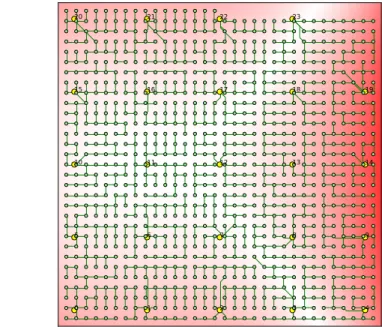
Finally, Figure 8 shows an example layout for 1000 nodes, where the turbines and substations are spaced roughly equally. We are reassured by the intuitive look of the result, where turbines are connected to nearby substations.

In summary, our algorithm has the following limitations:

– When associating turbines to substations, we do not know the real cost of as-sociating turbineti to substationsj, because this cost depends on the other

associations made. We approximate this cost byk(ti, sj), and find the best

turbine-to-substation associations using this approximation. These associa-tions remain fixed in the second part of the algorithm. It is not guaranteed that the associations obtained this way will lead to an optimal solution. – We solve the CMST problems using the EW heuristic, which gives good

solutions, but usually not optimal ones.

– Our resulting layouts may contain intersecting cables. This usually happens when there are not enough substations in an area.

We are not aware of any other attempts at solving the wind farm collector system design problem automatically at this scale. For this reason, we cannot compare our solution to work done by others. We hope that this algorithm will provide a baseline for comparing solutions in the future. Our algorithm may also be used to generate an initial feasible solution in a more advanced optimization process.

Fig. 6: Example layout for 24 substations, 976 turbines,nS= 42, andnC= 14.

Fig. 7: The same layout as in Figure 6, showing only the tree rooted at substation 12. There are few substations in the center-right area, so turbines are forced to make distant connections.

6. SOLUTIONS FOR MULTIPLE CABLE TYPES

Fig. 8: Example layout for 24 substations and 976 turbines that are conveniently located.nS = 42, andnC= 14.

6

Solutions for Multiple Cable Types

When there are multiple cable types, our problem does not map directly to existing problems in graph theory or network design. In this section, we describe our attempts at solving the Circuit Problem optimally. Our main result is the divide-and-conquer algorithm in section 6.4. The Substation and Full Problems with multiple cable types remain unexplored.

6.1 Exhaustively Listing all Trees

We started by exhaustively listing all possible trees for a given set of turbines, and evaluating each one in turn. According to Cayley’s formula [2], there arenn−2 possible spanning trees for a complete graph withnnodes. Pr¨ufer numbers [15] provide a one-to-one mapping between such trees and (n-2)-digit numbers, where each digit ranges from 1 to n. Rothlauf and Goldberg [17] describe the process of converting a Pr¨ufer number into a tree, and vice versa.

This method took about a minute forn= 8, slowing down quickly for larger n. We used it to validate the results of more advanced approaches.

6.2 Integer Linear Programming

Linear Programming is a mathematical method of optimizing a linear objective function, while satisfying a set of linear constraints. Linear programs are widely

used in business and economics, and there are a number of efficient algorithms for their solution. Unfortunately, if some variables have to be integers, then the problem becomes NP-hard.

We formulated the circuit problem as a linear program with binary and integer variables. The idea is to determine which cable type (if any) is used on each edge, and how much flow travels on that edge. An edge is represented as a triple (i, j, k), meaning an edge from ito j of capacityk. The set of all edges is E. If we have b cable types and n turbines, we have a total of bn2 possible edges. We denote the cost of edge (i, j, k) bycijk. Let binary variablexijk be 1

iff edge (i, j, k) is used, and integer variablefij represent the flow on that edge.

The problem is then to minimize: X (i,j,k)∈E cijk·xijk subject to: (i) X k k·xijk≥fij, ∀i, j (ii) X j fij− X j fji= 1, ∀i6= 0 (iii) X j fj0=n−1 (iv) X k xijk≤1, ∀i, j (v) xijk∈ {0,1} (vi) fij∈ {0,1, ..., nC}

Each turbine produces one unit of flow. Constraint (i) ensures that the cable used on edge (i, j) can accommodate the amount of flow on that edge. Constraint (ii) ensures the conservation of flow, and constraint (iii) ensures that all turbines are connected to the root. Constraint (iv) prevents placing multiple cables on the same edge. Finally, integrality constraints (v) and (vi) ensure that we get a valid solution.

Our formulation hasΘ(bn2) variables andΘ(bn2) constraints. We have used the lp solvelibrary to solve inputs with up to 8 turbines, but found it to be too slow beyond that. Interestingly, the time to find the solution depended a lot on what cost function was used. For a simpler cost function (KC(u, v, n) =

k(u, v) ifn≤2, k(u, v)·7 otherwise), we were able to solve inputs with up to 11 turbines.

6.3 Backtracking Algorithm

We developed an algorithm that builds the tree incrementally, in a fashion similar to Prim’s MST algorithm. At each step, an edge with flow information (u, v, n) is added to the current tree. We make sure that u is in the existing tree,v is not yet in the tree, and the new edge does not cause an overflow atu. We then

6. SOLUTIONS FOR MULTIPLE CABLE TYPES recurse, continuing to add edges until we have a full tree, or until the current tree is worse than the best complete tree seen so far. Upon returning from the recursion, we take the edge (u, v, n) back, and try another one. Our algorithm therefore follows the classical paradigm of backtracking search.

To avoid expanding poor branches, we developed a heuristic based on the MST. We use the same heuristic in the Divide-and-Conquer Algorithm, which we describe next. With the backtracking algorithm, we were able to solve inputs with up to 10 turbines.

6.4 Divide-and-Conquer Algorithm

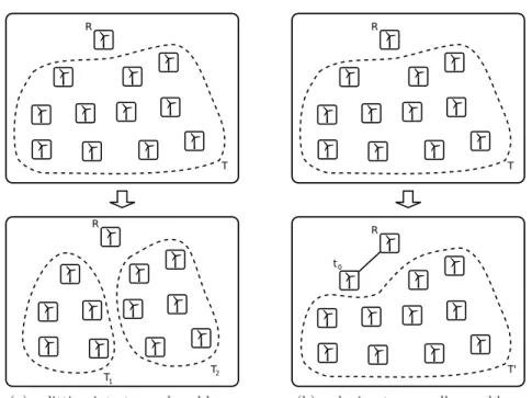
Our algorithm uses a divide-and-conquer approach with memoization. The main insight of the algorithm is that a circuit problem can be split into smaller circuit problems, and that the solutions to the smaller problems can be reused. 6.4.1 The Algorithm. We denote a problem by a tuple (R, T), whereR is a root node, andT is a set of nodes to be connected to the root. We denote the cost of a solution byC(R, T). The problem (R, T) can be divided in two ways:

– Partition the setT into two subsetsT1, T2, and solve the problems (R, T1) and (R, T2). The cost of solving the original problem is simply the sum of costs for the two subproblems: C(R, T) = C(R, T1) +C(R, T2). Figure 9a illustrates this.

– Pick a nodet0 ∈T, connect t0 to R, and solve the problem (t0, T′), where T′ = T \ {t0}. The cost of solving the original problem is the cost of the edge fromt0 to R, plus the cost of solving the smaller problem:C(R, T) = KC(t0, R,|T| −1) +C(t0, T′). Figure 9b illustrates this.

The base case is a single node, which requires no connections, and has cost zero. To solve a problem optimally, we divide it into subproblems in all possible ways, picking the one with the smallest cost. The solution for a subproblem can be used by multiple larger problems. To avoid repeated computation, we save the optimum cost, and the divide that leads to it, for each subproblem that we solve.

For a circuit of n nodes, there are n possible roots and 2n−1 _{possible sets} of turbines to connect to each root. The total number of subproblems is thus n·2n−1_{. This fits into memory comfortably forn= 14. However, time is still a} concern, because there are on the order of 2|T| _{ways of dividing each problem} (R, T) into subproblems. For this reason, we would like to “expand” as few subproblems as is required to guarantee that we find the optimal solution to the original circuit problem.

6.4.2 An Admissible Heuristic. We developed a heuristic to help us expand a subproblem only if it may lead to a cost better than the currently known best. The heuristic cost of solving subproblem (R, T), denoted byH(R, T), is obtained

R

T

T1

T2

R

(a) splitting into two subproblems

R

T

R

T' t0

(b) reducing to a smaller problem

Fig. 9: “Divide” step of the algorithm.

by computing the Minimum Spanning Tree of T ∪ {R}, and charging for one unit of flow on each edge. When dividing a problem into subproblems, we first compute the heuristic cost of solving the subproblems. If that results in a cost larger than the best cost known so far for the original problem, then we do not expand the subproblems.

This approach guarantees that we will find the optimum cost for a problemas long asthe heuristic never overestimates the true cost of solving a subproblem. In other words, the heuristic needs to be admissible: H(R, T)≤C(R, T). Our heuristic is admissible if a simple property holds for the cost function: The same amount of flow cannot cost more on a cheap edge than on an expensive edge: k(a, b)≤k(c, d)⇒KC(a, b, n)≤KC(c, d, n) for any flown.

The proof of admissibility is straightforward. Consider the problem (R, T). A solution is a spanning tree ofT∪{R}. Letn=|T|be the number of edges in such a spanning tree. Let (ai, bi) be the edges in the MST, sorted in increasing order

6. SOLUTIONS FOR MULTIPLE CABLE TYPES order by length. We have:

H(R, T) = n X i=1 KC(ai, bi,1) (1) ≤ n X i=1 KC(ci, di,1) (2) ≤ n X i=1 KC(ci, di, fi) =C(R, T) (3)

The first inequality holds becausek(ai, bi)≤k(ci, di) (otherwise we would

con-tradict the definition of the MST). The second inequality holds because the cost function on a particular edge is monotonically increasing with respect to flow. This proves that the heuristic is admissible:H(R, T)≤C(R, T). ⊓⊔

6.4.3 Empirical Evaluation. We have implemented this algorithm in Python, and validated it against the exhaustive search for small inputs (n= 7). We also ran our algorithm on randomly-generated inputs with n = 14, using the cost function described in section 4.2. Our turbines were distributed uniformly within the rectangle [0,1]×[0,1]. The terrain grid was given by the function:

1 +

4·(x−0.5)2−8·(y−0.3)3

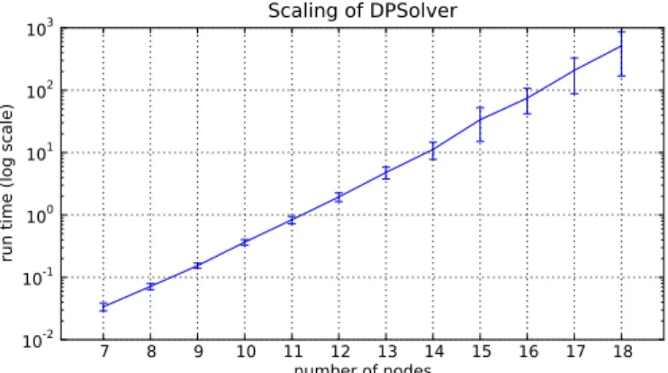
Figure 10 shows that the algorithm scales exponentially. For 14 turbines, the average runtime was 11.3 seconds, with a standard deviation of 3.5 seconds. For 15 turbines, the average was 33.7 seconds, with a 18.6-second standard deviation. (The time to precompute the pairwise costs was negligible.)

7 8 9 10 11 12 13 14 15 16 17 18_{number of nodes} 10-2 10-1 100 101 102 103

run time (log scale)

Scaling of DPSolver

Fig. 10: Scaling of the Divide-and-Conquer algorithm. 100 trials for n from 7 to 14; 20 trials for n from 15 to 18.

6.5 Summary

Our main result for multiple cable types is the divide-and-conquer algorithm presented above. It finds the optimal circuit for 14 turbines in less than a minute. For multiple cable types, the Substation and Full Farm Problems remain open.

7

When A Single Cable Type Is Good Enough

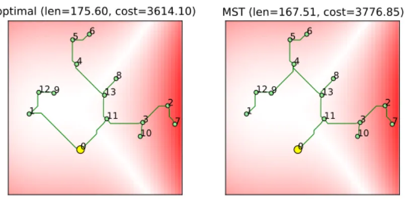
This section discusses under what circumstances a multiple-cable-types problem can be simplified to a type problem. Recall that for a single-cable-type Circuit Problem, the MST gives an optimal solution instantly. If we have multiple cable types, Figure 11 shows an example where the MST is not optimal. But if we compute the minimum spanning tree, and then evaluate the multiple-cable-types cost function on it, how far from optimal can it get? If it is close to optimal on average, then we can use the single-cable-type methods explored in section 5 to solve multiple-cable-types problems, without a large sacrifice in solution quality. 1 ₃ 2 4 5 6 7 8 9 10 11 12 ₁₃ 0

optimal (len=175.60, cost=3614.10)

1 ₃ 2 4 5 6 7 8 9 10 11 12 ₁₃ 0

MST (len=167.51, cost=3776.85)

Fig. 11: An example where the MST and the optimal circuit are not the same. Node 0 is the circuit root. The optimal circuit connects turbine 1 directly to the root, increasing the length of the tree, but reducing the overall cost, because fewer high-capacity cables are required. The length of the MST is 95.4% of the length of the optimal circuit, and the cost of the MST is 104.5% of the optimal circuit cost.

We found that with the cost function in section 4.2, the MST does very well. On 100 trials, the average ratio between the MST cost and the optimal tree cost was 1.023, with a standard deviation of 0.032. (We found the optimal tree using the algorithm from section 6.4.) We believe that the MST performs so well for

7. WHEN A SINGLE CABLE TYPE IS GOOD ENOUGH two reasons. Let’s take another look at our cost function:

KC(u, v, n) =        20·k(u, v) : n≤5 25·k(u, v) : n≤8 27·k(u, v) : n_≤12 41·k(u, v) : n_≤15

First, our cheapest cable can handle up to 5 turbines. Therefore, if all branches from the root of the MST have at most 5 turbines, then the MST is automatically optimal. Second, for up to 12 turbines, the cost of trenching dominates the cost of the actual cables ($15/ft compared to $5/ft, $7/ft, and $12/ft). The MST minimizes trenching length. Alternative trees likely lose more money on additional trenching length, than they gain by using thinner cables. We ran some more experiments to determine what factors affect this ratio.

7.1 The Effect of the Cost Function on MST Circuit Quality

We tested our default cost functionKC(u, v, n), and two additional cost functions

shown in Figure 12 in the Appendix. We used our original terrain grid, and 14 uniformly-distributed turbines. All statistics are based on 100 trials.

cost function mst/opt ratio run time (sec) mean stdev mean stdev KC (default) 1.023 0.032 11.3 3.5

KC1 (implausible) 2.255 0.348 30.0 5.1

KC2 (plausible) 1.112 0.076 48.0 9.7

KC1 is an unrealistic cost function, which does not exhibit economies of scale.

The function heavily penalizes branches with more than two turbines. This means that the optimal tree usually has many small branches, whereas the MST has fewer and larger branches. The MST is therefore a very poor solution. The average run time of the algorithm also increases, with respect to the original cost function.

KC2 does exhibit economies of scale, but the thinnest cable handles only two

turbines. The MST is not as good as it is for the original cost function, and the runtime increases even more.

We conclude that the cost function substantially affects the run time of the divide-and-conquer algorithm, and the quality of the MST circuit.

7.2 The Effect of the Terrain Grid on MST Circuit Quality

We tested several different grids, pictured in Figure 13 in the Appendix. Each grid had 50x50 cells. We used our original cost function KC(u, v, n), and 14

terrain grid functionmst/opt ratio run time (sec) mean stdev mean stdev G(default) 1.023 0.032 11.3 3.5

G1(hills) 1.015 0.022 12.3 4.0 G2 (uniform) 1.024 0.029 11.1 2.5 G3 (random) 1.023 0.031 11.5 3.0

We conclude that with our default cost function, the terrain grid does not substantially affect the running time of the divide-and-conquer algorithm, or the quality of the MST circuit.

7.3 The Effect of Turbine Placement on MST Circuit Quality We tested several schemes for placing turbines. In the ‘chain’ placement scheme, we place the turbines on a line with a random slope, and then perturb the position of each. In the ‘far’ placement scheme, we first place the circuit root, and then place the turbines randomly, making sure that no turbine is closer to the root than half the diagonal of the grid’s bounding rectangle. Figure 14 in the Appendix shows examples.

We used our original cost function and original terrain grid. All statistics are based on 100 trials.

turbine placement schememst/opt ratio run time (sec) mean stdev mean stdev uniform 1.023 0.032 11.3 3.5

chain 1.006 0.008 9.0 0.4 far 1.049 0.049 27.9 13.4

We conclude that different turbine placement schemes may affect running time, but do not significantly affect the quality of the MST circuit.

7.4 Summary and Discussion

Here is a summary of how the three factors affect the run time of the divide-and-conquer algorithm, and the quality of the MST circuit:

factor affects MST quality affects run time

cost function yes yes

turbine placement not significant yes terrain grid not significant not significant

The divide-and-conquer algorithm can thus be used to evaluate how “well-behaved” is the cost function in a multiple-cable-types problem. If the cost ratio between the MST and the optimal tree is close to 1 on average, then a good so-lution can be found using the single-cable-type soso-lutions in section 5. Otherwise, finding a good solution to the Full Farm remains an open problem.

8. CONCLUSION AND FUTURE WORK

8

Conclusion and Future Work

This paper makes three main contributions:

– We propose a model of the wind farm collector system design problem (sec-tion 2), and we decompose the problem into three layers: the Circuit, Sub-station, and Full Farm Problem (section 3).

– For the single-cable-type case, we present a greedy top-down algorithm for finding a feasible solution to the Full Farm Problem (section 5.2). The algo-rithm solves a min-cost flow problem to assign turbines to substations, and then uses the Esau-Williams heuristic to arrange each substation’s turbines into circuits. It scales up to 1000 turbines. Solutions given by this algorithm can be used as a baseline for comparing future algorithms, and as initial solutions in more advanced optimization schemes.

– For the multiple-cable-types case, we present a divide-and-conquer algorithm for finding an optimal solution to the Circuit Problem (section 6.4). This algorithm can be used to determine whether simplifying the problem to the single-cable-type case would result in a large or small sacrifice in solution cost (section 7.4).

There are many possible directions for future work:

Improving terrain modeling. Modeling a terrain with regions of different costs falls under the Weighted Region Problem (WRP). Our terrain grid (section 4) is a very simple solution, and Mitchell, Payton, and Keirsey [12] discuss some of its limitations. First of all, using a fine grid over a large area is inherently slow. Second, the grid causesdigitization biasdue to the fact that only rectilinear and diagonal path segments are allowed [12]. Using a better solution to the WRP could reduce running time and improve accuracy.

A more accurate cost function. Our cost function for multiple cable types (section 4.2) could be made more accurate by treating trenching cost, road con-struction cost, and cable cost separately.

Finding the optimal circuit faster in the multiple-cable-types case. An easy way to make our divide-and-conquer algorithm (section 6.4) faster is to rewrite it in C. We could also try formulating our Circuit Problem as a minimum-cost-flow problem. Our cost function would likely be concave (due to economies of scale), which makes the minimum-cost-flow problem NP-hard [6]. Another potentially useful related problem is the Fixed Charge Problem, where the cost function involves a fixed charge for using each edge, and a variable cost per unit flow: Cij(nij) = dij +kij ·nij. This problem is also NP-hard

[7]. Finally, two methods that appear often in the literature on combinatorial optimization are branch-and-bound, and Lagrangian relaxation. Both could be worth investigating.

Improving the Full Problem solution in the single-cable-type case. Our initial solution to the Full Problem (section 5.2) could be improved by using a more advanced CMST heuristic, instead of Esau-Williams. We could then take this initial solution, and try to improve it using stochastic search (hill climbing, tabu search, simulated annealing, evolutionary algorithms, etc).

Solving the Substation and Full Problems in the multiple-cable-types case. The Substation and Full Problems remain open in the multiple-cable-types case. Since even the small Circuit Problem is hard to solve deterministically in this case, we speculate that an evolutionary algorithm would be appropriate here.

Allowing arbitrary merge points. In our model, cables from different tur-bines can only be merged at a turbine or substation. In the real world, it might be possible to merge cables at arbitrary locations. This could reduce the total length of cable required, but it adds complexity to the problem. Approaches to the (NP-hard) Minimal Steiner Tree Problem [8] might apply.

Forbidding cable intersections. If overlapping cables are a problem when constructing real collector systems, we could investigate ways of disallowing in-tersecting edges in our algorithms.

Charging for branches. Our model does not incorporate the cost of branching cables at a turbine. If this cost is high, it might be better to have chains of turbines connected to a substation, instead of trees.

Choosing substation locations. All algorithms discussed in this paper as-sume that the substation locations are known. It would be useful to have an algorithm that finds good substation locations, either by picking from a list of candidates, or without any prior restrictions.

9

Acknowledgments

We are grateful to Nicholas Robinson (AWS OpenWind) for providing advice and knowledge of the domain. We also thank the MIT Summer Research Program for making this work possible.

References

1. Anita Amberg, Wolfgang Domschke, and Stefan Voß. Capacitated minimum span-ning trees: Algorithms using intelligent search, 1996.

2. A. Cayley. A theorem on trees. Quarterly Journal of Mathematics, 23:376–378, 1889.

9. ACKNOWLEDGMENTS

3. S. Dutta and T. J. Overbye. A clustering based wind farm collector system cable layout design. InPower and Energy Conference at Illinois (PECI), 2011 IEEE, pages 1–6, feb. 2011.

4. Bezalel Gavish. Topological design of telecommunication networks-local access design methods. Annals of Operations Research, 33:17–71, 1991. 10.1007/BF02061657.

5. Andrew V. Goldberg. An efficient implementation of a scaling minimum-cost flow algorithm. Journal of Algorithms, 22(1):1–29, 1997.

6. G. M. Guisewite and P. M. Pardalos. Algorithms for the single-source uncapaci-tated minimum concave-cost network flow problem. Journal of Global Optimiza-tion, 1:245–265, 1991. 10.1007/BF00119934.

7. Dorit S. Hochbaum and Arie Segev. Analysis of a flow problem with fixed charges.

Networks, 19(3):291–312, 1989.

8. F. K. Hwang and Dana S. Richards. Steiner tree problems.Networks, 22(1):55–89, 1992.

9. A. Kershenbaum. Computing capacitated minimal spanning trees efficiently.

Net-works, 4(4):299–310, 1974.

10. Gouveia L. and Lopes M. J. Using generalized capacitated trees for designing the topology of local access networks. Telecommunication Systems, 7:315–337, 1997. 11. Maine Mountain Power, LLC. Preliminary Engineering for the Black Nubble Wind

Farm 34.5 kV Collector System and 115 kV Interconnection Facility 54 MW Facil-ity. http://www.maine.gov/doc/lurc/projects/redingtonrevised/Documents/ Section01_Development_Description/Development_Electric/E_Pro_Reports/ 5.1_Electrical_Power_Line_Report.pdf, 2007.

12. Joseph S. B. Mitchell, David W. Payton, and David M. Keirsey. Planning and reasoning for autonomous vehicle control.International Journal of Intelligent Sys-tems, 2(2):129–198, 1987.

13. C. H. Papadimitriou. The complexity of the capacitated tree problem. Networks, 8(3):217–230, 1978.

14. R. C. Prim. Shortest connection networks and some generalizations. Bell System

Technology Journal, 36:1389–1401, 1957.

15. H. Pr¨ufer. Neuer beweis eines satzes ¨uber permutationen. Archiv f¨ur Mathematik

und Physik, 27:742–744, 1918.

16. G¨unther R. Raidl and Christina Drexel. A predecessor coding in an evolutionary al-gorithm for the capacitated minimum spanning tree problem. In Chris Armstrong, editor, Late Breaking Papers at the 2000 Genetic and Evolutionary Computation

Conference, pages 309-316, Las Vegas, NV, pages 309–316. 2000.

17. Franz Rothlauf and David Goldberg. Pruefer Numbers and Genetic Algorithms: A Lesson on How the Low Locality of an Encoding Can Harm the Performance of GAs. In Marc Schoenauer, Kalyanmoy Deb, Gnther Rudolph, Xin Yao, Evelyne Lutton, Juan Merelo, and Hans-Paul Schwefel, editors, Parallel Problem Solving

from Nature PPSN VI, volume 1917 ofLecture Notes in Computer Science, pages

A

Additional figures for the MST quality experiments

A. ADDITIONAL FIGURES FOR THE MST QUALITY EXPERIMENTS (a)G(x, y) = 1 +|4·(x−0.5)2 −8· (y−0.3)3 | (b) G1 (x, y) = 1 +|123 sin(10x) + 45 cos(8y)| (c)G2 = 1 (d)G3 =rand(1.0,2.0)

1 2 3_{45 6 7 8} 9 1011 _{12 13} 0

'chain' placement

'far' placement

Fig. 14: Examples of the ‘chain’ and ‘far’ turbine placements, with the optimal circuits shown.