remote sensing
ArticleA hybrid OSVM-OCNN Method for Crop
Classification from Fine Spatial Resolution Remotely
Sensed Imagery
Huapeng Li1,*, Ce Zhang2,3 , Shuqing Zhang1and Peter M. Atkinson4 1 Northeast Institute of Geography and Agroecology, Chinese Academy of Sciences,
Changchun 130000, China; [email protected]
2 Lancaster Environment Centre, Lancaster University, Lancaster LA1 4YQ, UK; [email protected] 3 Centre for Ecology & Hydrology, Library Avenue, Bailrigg, Lancaster LA1 4AP, UK
4 Faculty of Science and Technology, Lancaster University, Lancaster LA1 4YR, UK; [email protected] * Correspondence: [email protected]; Tel.:+86-0431-85542230
Received: 20 August 2019; Accepted: 11 October 2019; Published: 12 October 2019 Abstract:Accurate information on crop distribution is of great importance for a range of applications including crop yield estimation, greenhouse gas emission measurement and management policy formulation. Fine spatial resolution (FSR) remotely sensed imagery provides new opportunities for crop mapping at a detailed level. However, crop classification from FSR imagery is known to be challenging due to the great intra-class variability and low inter-class disparity in the data. In this research, a novel hybrid method (OSVM-OCNN) was proposed for crop classification from FSR imagery, which combines a shallow-structured object-based support vector machine (OSVM) with a deep-structured object-based convolutional neural network (OCNN). Unlike pixel-wise classification methods, the OSVM-OCNN method operates on objects as the basic units of analysis and, thus, classifies remotely sensed images at the object level. The proposed OSVM-OCNN harvests the complementary characteristics of the two sub-models, the OSVM with effective extraction of low-level within-object features and the OCNN with capture and utilization of high-level between-object information. By using a rule-based fusion strategy based primarily on the OCNN’s prediction probability, the two sub-models were fused in a concise and effective manner. We investigated the effectiveness of the proposed method over two test sites (i.e., S1 and S2) that have distinctive and heterogeneous patterns of different crops in the Sacramento Valley, California, using FSR Synthetic Aperture Radar (SAR) and FSR multispectral data, respectively. Experimental results illustrated that the new proposed OSVM-OCNN approach increased markedly the classification accuracy for most of crop types in S1 and all crop types in S2, and it consistently achieved the most accurate accuracy in comparison with its two object-based sub-models (OSVM and OCNN) as well as the pixel-wise SVM (PSVM) and CNN (PCNN) methods. Our findings, thus, suggest that the proposed method is as an effective and efficient approach to solve the challenging problem of crop classification using FSR imagery (including from different remotely sensed platforms). More importantly, the OSVM-OCNN method is readily generalisable to other landscape classes and, thus, should provide a general solution to solve the complex FSR image classification problem.
Keywords: crop mapping; object-based image classification; deep learning; decision fusion; FSR remotely sensed imagery
1. Introduction
Accurate crop distribution information from regional-to-global scales is essential for estimating crop yield [1], modelling greenhouse gas (GHG) emissions from agriculture [2] and making effective
Remote Sens.2019,11, 2370 2 of 20
agrarian management policies [3]. Moreover, agricultural ecosystems are often managed intensively and modified frequently [4], which might alter land cover/use patterns rapidly and, thus, influence ecological processes and biogeochemical cycles [5]. These spatial and temporal characteristics pose a great challenge for traditional approaches (e.g., ground surveys) to monitoring agricultural systems. Remote sensing using sensors onboard satellite and aircraft platforms, however, has been shown to be an effective means of crop monitoring at regional-to-global scales, and has the advantages of being consistent, timely and cost-efficient (e.g., [2,5]).
Coarse and medium spatial resolution multispectral data, such as Landsat, SPOT and MODIS (Moderate Resolution Imaging Spectroradiometer), have been used widely for crop classification and mapping [3,6,7]. However, the accuracy of crop maps generated from these images is inevitably compromised by the spatial limitation [8], especially over the highly fragmented and heterogeneous agricultural areas. As stated by [9], a spatial resolution of less than 10 m is required for precision agriculture. More recently, remotely sensed imagery from fine spatial resolution (FSR) (<10 m) satellite systems (e.g., RapidEye, IKONOS, and WorldView) as well as airborne systems (e.g., Uninhabited Aerial Vehicle Synthetic Aperture Radar (UAVSAR)) is now available commercially, providing new opportunities for crop classification and mapping in very fine detail [9,10]. However, high intra-class variance and low inter-class separability over croplands in FSR images may exist because of differences in climatic conditions, topographic properties, soil composition, farming practices and so on [11]. Moreover, FSR imagery has fewer multispectral bands (around four) in comparison to medium resolution data (e.g., MODIS and Landsat), which leads to subtle differences in spectral/polarimetric properties amongst crop types (i.e., crop types are difficult to discriminate). Therefore, developing advanced classification methods for accurate crop mapping and monitoring is of prime concern, especially with a view to exploiting the deep hierarchical features presented in FSR imagery.
During the past few decades, a vast array of methods has been developed for remote sensing image classification [12–14]. These methods can be categorised into pixel-based and object-based methods according to the basic unit of analysis (either per-pixel or per-object) [15]. Pixel-based classification methods that rely purely upon spectral (or polarimetric) signatures have been used widely for crop classification using various types of imagery (including the newly-launched Sentinel-2 imagery [16–18]). However, these methods often produce limited classification accuracy due to large intra-class variances as stated above. Severe salt-and-pepper effects may occur owing to the noise in FSR imagery. Although some post-classification algorithms (e.g., spatial filters) might alleviate the noise to some extent, they may also erase small objects of interest comprised of just a few pixels. Compared with pixel-wise algorithms, object-based image analysis (OBIA) built upon segmented homogeneous objects [15] is preferable for crop classification using FSR remotely sensed images (e.g., [19,20], in which objects instead of pixels are adopted as the basic unit of analysis. This allows spatial information (e.g., texture, shape) with respect to the objects to be incorporated into the classification process, thus, reducing the salt-and-pepper noise [15].
Under the framework of OBIA, machine learning algorithms (e.g., the support vector machine (SVM), the multilayer perceptron (MLP) and the random forest (RF)) have been used for crop classification and mapping thanks to their ability to deal with multi-modal and noisy data [21]. The SVM, as a typical non-parametric machine learning classifier, was often found to outperform other machine learning algorithms in image classification due to its high generalisation ability [22]. The objected-based SVM (OSVM) has, thus, been popular for complex crop classification tasks [2,23]. In the OBIA classification process, there are generally two kinds of information that can be obtained from a spatially segmented region: within-object information (such as spectra, polarization, texture) and between-object information (such as configuration and topological relationships between adjacent objects) [24]. The OSVM classifier can extract within-object features (low-level information) from FSR images for classification. However, it is essentially a single-layer classifier (linear SVM) or two-layer classifier (kernel SVM) [25], which might overlook the high-level between-object information that may be critical to crop identification. For example, crop swath direction conveys important information
for the identification of crop pattern [26]. In this context, a series of object-based spatial contextual descriptive indicators were developed based on spatial metrics, graphs and ontologies [27,28] to derive high-level semantic information from FSR images. However, it is often very difficult to characterise the spatial contexts as a set of “rules” in view of the structurally complicated and diverse agricultural landscapes [2], even if these complex spatial patterns might be interpreted by human experts [29].
Recent developments in artificial intelligence and pattern recognition demonstrated that high-level feature representations can be extracted with multi-layer neural networks in an “end-to-end” manner without using human-crafted “rules” [30]. These breakthrough deep learning algorithms achieved unprecedented success in a wide range of challenging domains, such as speech recognition, visual object recognition and target detection [30,31]. As a representative deep learning method, convolutional neural networks (CNNs) have drawn a lot of academic and industrial interest, and made huge improvements in the field of image analysis, such as text recognition [32], speech detection [31] and image denoising [33]. CNNs, with great capability in high-level feature characterization, were also applied to various remote sensing applications, such as object detection [34], image segmentation [35] and scene classification [36]. In addition, CNN-based approaches have been developed to solve the complex problem of remote sensing classification, where all pixels in an image are labelled into several categories. For example, Stoian, et al. [37] presented a fully-realized CNN model for land cover classification using multi-temporal high spatial resolution imagery. Chen, et al. [25] proposed a three-dimensional (3D) CNN for hyperspectral image classification by using both spectral and spatial features. Recently, Zhang, et al. [38] provided a novel approach by combining CNNs with rough sets for classification of FSR images. The above-mentioned work has achieved promising classification results, demonstrating the advantages of CNNs with respect to spatial feature representation. However, these pixel-based CNNs classify images by applying contextual patches as inputs, which often blurs the boundaries between adjacent ground objects, leading to over-smooth classification results [38]. To overcome this problem, a new object-based CNN (OCNN) framework was presented which combined the OBIA and CNN techniques, such that the segmented objects can be identified while retaining precise boundary information [24]. The OCNN method was applied to the complex land use classification task and produced encouraging classification results. However, with a fix-sized input window (receptive field), large uncertainties may be introduced into the OCNN classification process, especially for those objects with areas far smaller or larger than the input window [24]. Moreover, while the CNN model can explore the high-level features hidden in remotely sensed images, low-level features (e.g., within-object spectra) observed by shallow models may be overlooked [38].
Any single classifier is unlikely to achieve promising results if the scenes of remotely sensed imagery are complex [38,39]. The combination of multiple classification methods with complementary behaviours would be a good idea to improve complex land cover classification [40] and crop classification [39], by better exploring the minute differences that may exist between the classes. Within the remote sensing community, there are generally three types of ensemble-based systems, namely “consensus classification”, “multiple classifier systems” and “decision fusion” [41]. Relying on multiple types of datasets, the utility of consensus classification is constrained due to the lack of availability of such data. By means of manipulating training samples to generate subsets randomly (boosting and bagging) [42], multiple classifier systems require extremely large sample sizes and deliver high time complexity. In contrast, decision fusion that combines the outputs of individual classifiers with a certain fusion rule to take advantage of complementary characteristics is a generally effective ensemble strategy [40]. For example, different classifiers may produce accurate results over different areas within a classification map and, hence, produce complementary results [38]. However, the above-mentioned ensemble methods are always performed based on pixel-wise classifiers with shallow structures and, thus, are not well suited to cope with the complex FSR image classification problem.
In this research, a novel OSVM-OCNN approach was proposed by combining the OSVM (an object-based SVM model with shallow architectures) and the OCNN (an object-based CNN model with deep architectures) through a rule-based decision fusion strategy. Image segmentation was first
Remote Sens.2019,11, 2370 4 of 20
used to partition the agricultural landscape into basic crop patches (objects), based on whether the SVM and CNN models were respectively applied to allocate a label to each object. The outputs of the two models were combined subsequently through a rule-based fusion strategy according to prediction probability output from the CNN. Such a fusion decision strategy allows the rectification of CNN predictions with low confidence using SVM predictions at the object level. The major contributions of this research can be summarised as: (1) the shallow architecture SVM and the deep architecture CNN was first found to be complementary to each other in terms of crop classification at the object level; (2) a straightforward rule-based decision fusion strategy was developed to effectively fuse the results of the OSVM and OCNN. We investigated the effectiveness of the proposed approach over two study sites with heterogeneous agriculture landscapes in California, USA, using the FSR UAVSAR and RapidEye imagery.
The reminder of this paper is organised into five sections: Section2elaborates the proposed methods in detail. Section3provides the study area, datasets, model structure and experimental results. A thorough discussion of the observed results is made in Section4, and the conclusions of this research are drawn in Section5.
2. Method
2.1. Overview of the Support Vector Machine (SVM)
The principle of the SVM is to determine an optimal classification hyperplane by which a maximum margin can be achieved to separate the dataset into a predefined number of classes [43]. In this case, a kernel function, with additional variables, is usually adopted to map the non-linear input vectors into a higher space (e.g., Euclidean)Φ(X).
Suppose there is a set of data(x1,y1),(x2,y2),. . .,(xm,ym)distributed in the multi-dimensional feature spaceX, wherexi denotes a sample vector with yi ∈ {−1,+1}as the corresponding target.
The hyperplane in the transformed space can be defined as follows:
f(x) =ω·Φ(x) +b (1)
whereωdenotes the weight vector of the hyperplane, andbrepresents the offset of the hyperplane. The SVM cost function is defined using the following equations:
minω,b,εJ(ω,b,ε) = 1 2||ω|| 2+C m X i=1 εi (2) subject to: yiωxTi·xj+b≥1−εi,i=1,. . .,m. (3)
whereεidenotes the slack variables, andCrefers to the penalty parameter used to control the trade-off between empirical risk and model complexity.
2.2. Overview of Convolutional Neural Networks (CNNs)
The CNN is a forward neural network that includes an input layer, multi-hidden layers and output layer, which are connected to each other with the output of the previous layer being the input of the next layer. High-level features contained in the raw data are extracted gradually through implementation of both a convolutional layer and a pooling/subsampling layer. To learn nonlinear representations of input data, a nonlinear activation function (e.g., sigmoid, rectified linear units) is adopted [31]. In general, the operations performed in a CNN can be summarised as:
where Ol−1represents the input to thelth layer,wl andblare the weights and biases of the layer, respectively,σ(·)indicates the non-linearity function and the symbol∗denotes linear convolution;
a pooling operation (poolp) with a window sizep is often performed following the convolution operation to extract invariant features of the input map, forming the output (Ol) of the current (lth) layer.
The feature maps outputted by the last pooling layer are then flattened into a one-dimensional array and classified using a logistic regression (LR). A softmax activation function is employed in the LR to ensure the prediction probability of each output unit belonging to a certain class sums to one.
2.3. Hybrid Object-based SVM and CNN (OSVM-OCNN) Approach
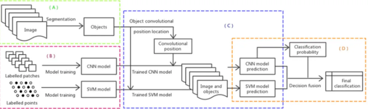
We propose a novel hybrid object-based SVM and CNN (OSVM-OCNN) approach for crop classification from FSR remotely sensed imagery. In brief, the trained SVM and CNN models were used to predict the class of each segmented object, respectively, and a fusion strategy was applied subsequently to combine the two classifications to achieve the final classification map. Figure1shows the workflow of the presented OSVM-OCNN methodology, which comprises four steps, namely (1) image segmentation, (2) SVM and CNN model training, (3) SVM and CNN model inference and (4) decision fusion of SVM and CNN predictions, details of which will be elaborated in the following sections.
Remote Sens. 2019, 11, 2370 5 of 20
where O represents the input to the 𝑙th layer, 𝑤 and 𝑏 are the weights and biases of the layer, respectively, 𝜎(∙) indicates the non-linearity function and the symbol ∗ denotes linear convolution; a pooling operation (pool ) with a window size 𝑝 is often performed following the convolution operation to extract invariant features of the input map, forming the output (O) of the current (𝑙th) layer.
The feature maps outputted by the last pooling layer are then flattened into a one-dimensional array and classified using a logistic regression (LR). A softmax activation function is employed in the LR to ensure the prediction probability of each output unit belonging to a certain class sums to one.
2.3. Hybrid Object-based SVM and CNN (OSVM-OCNN) Approach
We propose a novel hybrid object-based SVM and CNN (OSVM-OCNN) approach for crop classification from FSR remotely sensed imagery. In brief, the trained SVM and CNN models were used to predict the class of each segmented object, respectively, and a fusion strategy was applied subsequently to combine the two classifications to achieve the final classification map. Figure 1 shows the workflow of the presented OSVM-OCNN methodology, which comprises four steps, namely (1) image segmentation, (2) SVM and CNN model training, (3) SVM and CNN model inference and (4) decision fusion of SVM and CNN predictions, details of which will be elaborated in the following sections.
Figure 1. Flowchart illustrating the presented object-based support vector machine-object-based convolutional neural network (OSVM-OCNN) method with four major steps: (A) image segmentation, (B) model training, (C) model inference and (D) fusion decision.
2.3.1. Image Segmentation
Image segmentation is considered the fundamental step of the OSVM-OCNN as the prediction procedures of both SVM and CNN modules are based on segmented image objects (Figure 1). In this research, the widely used multi-resolution segmentation (MRS) algorithm was adopted to partition the imagery into crop patches (i.e., objects) with spectrally and spatially homogeneous information [44]. For the fully polarimetric UAVSAR data, three raw linear polarizations (bands HH, HV, VV) together with polarimetric parameters from the Cloude-Pottier (entropy, anisotropy, and alpha angle) and Freeman-Durden (fractions of double-bounce, single-bounce, and volume scatters) decompositions [45,46] were combined as input data for image segmentation. As for the optical RapidEye imagery, all five multispectral (Blue, Green, Red, Red Edge and Near Infrared) bands were used as input for segmentation.
2.3.2. SVM and CNN Model Training
In this research, the radial basis function (RBF) SVM was selected owing to its capacity to address complicated non-linear classification problems [47]. The SVM model was trained using the spectral (or polarimetric) information within the segmented patches. Two types of feature were extracted from each object for classification, including the mean and standard deviation of feature bands. All
Figure 1. Flowchart illustrating the presented object-based support vector machine-object-based convolutional neural network (OSVM-OCNN) method with four major steps: (A) image segmentation, (B) model training, (C) model inference and (D) fusion decision.
2.3.1. Image Segmentation
Image segmentation is considered the fundamental step of the OSVM-OCNN as the prediction procedures of both SVM and CNN modules are based on segmented image objects (Figure 1). In this research, the widely used multi-resolution segmentation (MRS) algorithm was adopted to partition the imagery into crop patches (i.e., objects) with spectrally and spatially homogeneous information [44]. For the fully polarimetric UAVSAR data, three raw linear polarizations (bands HH, HV, VV) together with polarimetric parameters from the Cloude-Pottier (entropy, anisotropy, and alpha angle) and Freeman-Durden (fractions of double-bounce, single-bounce, and volume scatters) decompositions [45,46] were combined as input data for image segmentation. As for the optical RapidEye imagery, all five multispectral (Blue, Green, Red, Red Edge and Near Infrared) bands were used as input for segmentation.
2.3.2. SVM and CNN Model Training
In this research, the radial basis function (RBF) SVM was selected owing to its capacity to address complicated non-linear classification problems [47]. The SVM model was trained using the spectral (or polarimetric) information within the segmented patches. Two types of feature were extracted from each object for classification, including the mean and standard deviation of feature bands. All these
Remote Sens.2019,11, 2370 6 of 20
object-based hand-crafted features were fed into the SVM model for classification. Different from the SVM model, the image patches used to train the CNN model were extracted using a pre-defined square input window rather than segmented patches. The input window size and a range of parameters of the CNN model were tuned empirically, as detailed in Section3.
The trained SVM and CNN models were used for the following model interference. 2.3.3. SVM and CNN Model Inference
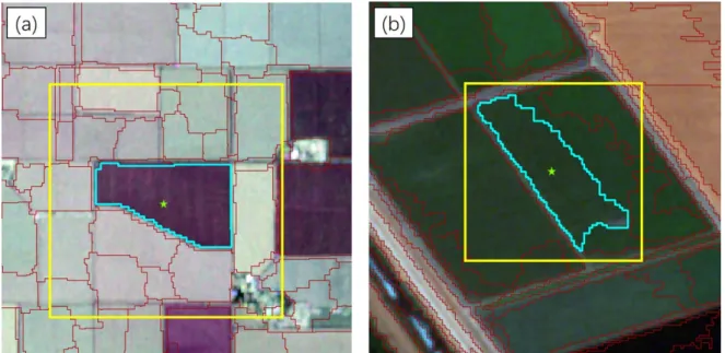
At the model inference stage, the trained SVM was used directly to predict the label of each segmented object based on the hand-crafted features mentioned above. The inference procedure of the CNN model consists of two steps: the convolutional position of an object was first located to acquire the input image patch of CNN; then, the label of the object was predicted with the trained CNN model with the located convolutional positions and input image patches. To acquire representative features of crop patches, the object convolutional position should be located at the centre of each object. In this research, the convolutional position of each object was determined by its geometric centroid [48]. Figure2provides two examples of object convolutional position location.
For a specific object, its crop class is inferred by the trained CNN model; at the same time, the SVM model also allocates a class label to the object. Thus, each object has two predictions coming from the SVM and CNN models.
Remote Sens. 2019, 11, 2370 6 of 20
these object-based hand-crafted features were fed into the SVM model for classification. Different from the SVM model, the image patches used to train the CNN model were extracted using a pre-defined square input window rather than segmented patches. The input window size and a range of parameters of the CNN model were tuned empirically, as detailed in Section 3.
The trained SVM and CNN models were used for the following model interference. 2.3.3. SVM and CNN Model Inference
At the model inference stage, the trained SVM was used directly to predict the label of each segmented object based on the hand-crafted features mentioned above. The inference procedure of the CNN model consists of two steps: the convolutional position of an object was first located to acquire the input image patch of CNN; then, the label of the object was predicted with the trained CNN model with the located convolutional positions and input image patches. To acquire representative features of crop patches, the object convolutional position should be located at the centre of each object. In this research, the convolutional position of each object was determined by its geometric centroid [48]. Figure 2 provides two examples of object convolutional position location.
For a specific object, its crop class is inferred by the trained CNN model; at the same time, the SVM model also allocates a class label to the object. Thus, each object has two predictions coming from the SVM and CNN models.
Figure 2. Two examples to illustrate the convolutional position (green star) of a specific object (highlighted cyan polygon) as well as the corresponding convolutional input window (yellow rectangle); the other segmented patches are delineated by red polygons. (a) and (b) demonstrate a subset of the Uninhabited Aerial Vehicle Synthetic Aperture Radar (UAVSAR) and RapidEye imagery, respectively. Details of the two types of images employed here are provided in Section 3.
2.3.4. Decision Fusion of the SVM and CNN Models
For each object, the predictions of the SVM and CNN models are 𝑚-dimensional vectors 𝑃 =
(𝑝 , 𝑝 , … , 𝑝 ), where 𝑚 is the number of classes, and each dimension 𝑖 ∈ [1,2, … , 𝑚] denotes the
predictive probability of the 𝑖th class. Ideally, the prediction probability should be 1 for the target
class and 0 for the others. However, this is not likely to happen in consideration of the complexity of
remotely sensed data. The probability for each class can be represented as 𝑓(𝑥) = {𝑝 |𝑥 ∈ [1,2, … , 𝑚]},
where 𝑝 ∈ [0,1] and ∑ 𝑝 = 1. The SVM and CNN models simply classify each object into the class
with the maximum membership (class(𝐶)) across all classes as follows:
class(𝐶) = argmax({𝑓(𝑥) = 𝑝 |𝑥 ∈ [1,2, … , 𝑚]}) (5)
Figure 2. Two examples to illustrate the convolutional position (green star) of a specific object (highlighted cyan polygon) as well as the corresponding convolutional input window (yellow rectangle); the other segmented patches are delineated by red polygons. (a) and (b) demonstrate a subset of the Uninhabited Aerial Vehicle Synthetic Aperture Radar (UAVSAR) and RapidEye imagery, respectively. Details of the two types of images employed here are provided in Section3.
2.3.4. Decision Fusion of the SVM and CNN Models
For each object, the predictions of the SVM and CNN models are m-dimensional vectors
P= (p1,p2,. . .,pm), wheremis the number of classes, and each dimensioni∈[1, 2,. . .,m]denotes the predictive probability of theith class. Ideally, the prediction probability should be 1 for the target class and 0 for the others. However, this is not likely to happen in consideration of the complexity of remotely sensed data. The probability for each class can be represented as f(x) =px
wherepx∈[0, 1]andPm
1 px=1. The SVM and CNN models simply classify each object into the class with the maximum membership (class(C)) across all classes as follows:
class(C) =argmaxf(x) =px
x∈[1, 2,. . .,m]
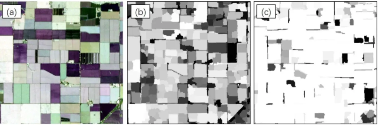
(5) For a specific segmented object, the SVM model uses only the features that fall completely within the object (within-object information) for classification. As a result, objects with distinctive low-level features (e.g., light regions in Figure3b) can be separated easily by the SVM, regardless of the size of objects. However, SVMs cannot identify accurately those objects with similar within-object features (e.g., dark regions in Figure3b), due to the lack of contextual information in the classification process. In contrast, the CNN model can extract deep high-level features (between-object information) for classification and, thus, is superior to the SVM in identifying complex objects. Note that the CNN uses a pre-defined square input window to extract features and predict labels of objects. As a result, for a specific patch, there are two situations to consider: (1) if the size of the target object (e.g., small-sized) mismatches with the scale of input window (i.e., a large area of other crop types as contextual information in the input window), the prediction probability of the object tends to be low (e.g., dark patches in Figure3c); (2) if the input window covers only a homogeneous region, the probability tends to be large (e.g., light patches in Figure3c).
Remote Sens. 2019, 11, 2370 7 of 20
For a specific segmented object, the SVM model uses only the features that fall completely within the object (within-object information) for classification. As a result, objects with distinctive low-level features (e.g., light regions in Figure 3b) can be separated easily by the SVM, regardless of the size of objects. However, SVMs cannot identify accurately those objects with similar within-object features (e.g., dark regions in Figure 3b), due to the lack of contextual information in the classification process. In contrast, the CNN model can extract deep high-level features (between-object information) for classification and, thus, is superior to the SVM in identifying complex objects. Note that the CNN uses a pre-defined square input window to extract features and predict labels of objects. As a result, for a specific patch, there are two situations to consider: (1) if the size of the target object (e.g., small-sized) mismatches with the scale of input window (i.e., a large area of other crop types as contextual information in the input window), the prediction probability of the object tends to be low (e.g., dark patches in Figure 3c); (2) if the input window covers only a homogeneous region, the probability tends to be large (e.g., light patches in Figure 3c).
Figure 3. (a) A subset of the UAVSAR image (bands VV, HV and HH) used in this paper, (b) the prediction probability generated by the OSVM model, (c) the prediction probability achieved by the OCNN model. Note that the white objects denote high predictive probability, while dark objects represent low probability.
In light of the above-mentioned complementarities of the SVM and CNN, a rule-based fusion strategy can be presented to combine the two models for increased classification accuracy. The fusion output gives credit to the CNN if its prediction probability is greater than or equal to a predefined threshold (𝛼); otherwise, it trusts the output of the SVM. Assume an image is segmented into 𝑁 objects. For a given segmented object (𝑂), where 𝑖 = 1,2, … , 𝑁, a decision fusion strategy can be formulated to determine the class label (𝑐𝑙𝑎𝑠𝑠(𝑂 )) of the object as follows:
𝑐𝑙𝑎𝑠𝑠(𝑂 ) = 𝑐𝑙𝑎𝑠𝑠 𝑝𝑟𝑜𝑏 ≥ 𝛼
𝑐𝑙𝑎𝑠𝑠 𝑜𝑡ℎ𝑒𝑟𝑤𝑖𝑠𝑒 (6)
where 𝑐𝑙𝑎𝑠𝑠 and 𝑐𝑙𝑎𝑠𝑠 denote the predictions of the CNN and SVM models, respectively, and
𝑝𝑟𝑜𝑏 represents the probability of the predicted class for the object 𝑖 achieved by the CNN
model. Here, the threshold (𝛼) is estimated using a grid search approach [49], that is, the threshold with the greatest classification accuracy is regarded as the optimal 𝛼.
To test the performance of the proposed OSVM-OCNN method, four benchmarks including the object-based SVM (OSVM), object-based CNN (OCNN), pixel-based SVM (PSVM) and pixel-based CNN (PCNN) were compared in this research.
3. Experimental Results
3.1. Study Area and Data
In this research, two typical crop areas (Figure 4), S1 and S2, located in the middle of the Sacramento Valley, in northern California were selected as case study sites. California is considered as a productive agricultural state in the United States, and accounts for about 15% of national receipts
Figure 3. (a) A subset of the UAVSAR image (bands VV, HV and HH) used in this paper, (b) the prediction probability generated by the OSVM model, (c) the prediction probability achieved by the OCNN model. Note that the white objects denote high predictive probability, while dark objects represent low probability.
In light of the above-mentioned complementarities of the SVM and CNN, a rule-based fusion strategy can be presented to combine the two models for increased classification accuracy. The fusion output gives credit to the CNN if its prediction probability is greater than or equal to a predefined threshold (α); otherwise, it trusts the output of the SVM. Assume an image is segmented intoNobjects. For a given segmented object (Oi), wherei=1, 2,. . .,N, a decision fusion strategy can be formulated to determine the class label (class(Oi)) of the object as follows:
class(Oi) = (
classcnn probcnni ≥α
classsvm otherwise (6)
whereclasscnn andclasssvmdenote the predictions of the CNN and SVM models, respectively, and
probcnni represents the probability of the predicted class for the objectiachieved by the CNN model. Here, the threshold (α) is estimated using a grid search approach [49], that is, the threshold with the greatest classification accuracy is regarded as the optimalα.
To test the performance of the proposed OSVM-OCNN method, four benchmarks including the object-based SVM (OSVM), object-based CNN (OCNN), pixel-based SVM (PSVM) and pixel-based CNN (PCNN) were compared in this research.
Remote Sens.2019,11, 2370 8 of 20
3. Experimental Results 3.1. Study Area and Data
In this research, two typical crop areas (Figure4), S1 and S2, located in the middle of the Sacramento Valley, in northern California were selected as case study sites. California is considered as a productive agricultural state in the United States, and accounts for about 15% of national receipts for crops [50]. The two study sites are heterogeneous and different from each other in crop composition, thus, being ideal to test remote sensing image classification algorithms. Based on the Crop Data Layer (CDL) produced by the United States Department of Agriculture (USDA) [51], 10 dominant crop classes were found within S1 (Table1), including walnut, almond, alfalfa, hay, clover, winter wheat, corn, sunflower, tomato and pepper, and nine major crop classes (Table1) in S2, namely walnut, almond, fallow, alfalfa, winter wheat, corn, sunflower, tomato and cucumber.
Remote Sens. 2019, 11, 2370 8 of 20
for crops [50]. The two study sites are heterogeneous and different from each other in crop composition, thus, being ideal to test remote sensing image classification algorithms. Based on the Crop Data Layer (CDL) produced by the United States Department of Agriculture (USDA) [51], 10 dominant crop classes were found within S1 (Table 1), including walnut, almond, alfalfa, hay, clover, winter wheat, corn, sunflower, tomato and pepper, and nine major crop classes (Table 1) in S2, namely walnut, almond, fallow, alfalfa, winter wheat, corn, sunflower, tomato and cucumber.
Figure 4. The two study sites S1 and S2 over the agricultural district of the Sacramento Valley, California.
In S1, the Uninhabited Aerial Vehicle Synthetic Aperture Radar (UAVSAR) image was captured on 29 August 2011 (the peak biomass stage). The UAVSAR, an airborne polarimetric interferometric radar system, is operated in L-band with a wavelength of 23.84 cm [52]. The range and azimuth pixel spacings in single look complex imagery are 1.66 m and 1 m, respectively. The UAVSAR used in S1 is in the GRD format (georeferenced), in which the calibrated complex data were multilooked and projected to the ground coordinate. The data has a fine spatial resolution of 5 m and a spatial extent of 3474 × 2250 pixels. No additional filter algorithms were applied to the image, since multiplicative noise was reduced by the multilook procedure [53]. Three raw linear polarizations (HH, HV and VV), as well as six parameters (stated in Section 2.3.1) from the Cloude-Pottier and Freeman-Durden decompositions, were extracted for crop classification.
In S2, a cloud-free RapidEye image (Level 3A Ortho product) was acquired on 10 July 2016. RapidEye is a constellation of five satellites that are equally spaced in the same orbital plane, producing a ground sampling distance (GSD) of 6.5 m at nadir [54]. The RapidEye imagery used in S2 is Ortho product, with sensor, radiometric and geometric correction using level 1 digital terrain elevation data, was delivered resampled to a spatial resolution of 5 m. The image employed in this research has a spatial extent of 3222 × 2230 pixels and five optical bands, namely blue (440–550 nm), green (520–590 nm), red (630–685 nm), red edge (690–730 nm) and near infrared (760–850). To obtain surface reflectance, the image was atmospherically corrected using the atmospheric and topographic correction method supported by the ERDAS IMAGINE software.
We acquired sample points from the USDA-CDL data by means of stratified random sampling. The CDL data are widely used as a ground reference owing to their very high quality [10,55]. Patches of major crop types in each site were outlined [10] and split randomly into two equal subsets. A 50% subset was for training samples generation, and the other 50% subset for testing samples collection, so as to make sure that training and testing samples come from different crop patches. To acquire enough representative samples, the sample size for each crop class was set at around 200 over the two study sites (Table 1). A total number of 2268 and 2020 samples were acquired for S1 and S2, respectively. Note that 80% of the training samples were used to train individual classification methods and the remaining 20% (validation set) were employed to select the optimal hyper-parameters of the classifiers.
Figure 4.The two study sites S1 and S2 over the agricultural district of the Sacramento Valley, California.
Table 1.Number of collected samples for each crop class over the two study sites.
Study Sites Crop Class Number of Objects Training Sample Testing Sample Total Sample
S1 Walnut 31 112 112 224 Almond 33 110 110 220 Alfalfa 55 125 125 250 Hay 26 101 101 202 Clover 41 110 110 220 Winter wheat 68 120 120 240 Corn 45 108 108 216 Sunflower 47 122 122 244 Tomato 58 120 120 240 Pepper 32 106 106 212 S2 Walnut 39 108 108 216 Almond 45 115 115 230 Fallow 30 90 90 180 Alfalfa 35 124 124 248 Winter wheat 40 116 116 232 Corn 22 93 93 186 Sunflower 57 130 130 260 Tomato 63 141 141 282 Cucumber 21 93 93 186
In S1, the Uninhabited Aerial Vehicle Synthetic Aperture Radar (UAVSAR) image was captured on 29 August 2011 (the peak biomass stage). The UAVSAR, an airborne polarimetric interferometric radar system, is operated in L-band with a wavelength of 23.84 cm [52]. The range and azimuth pixel spacings in single look complex imagery are 1.66 m and 1 m, respectively. The UAVSAR used in S1 is in the GRD format (georeferenced), in which the calibrated complex data were multilooked and
projected to the ground coordinate. The data has a fine spatial resolution of 5 m and a spatial extent of 3474×2250 pixels. No additional filter algorithms were applied to the image, since multiplicative
noise was reduced by the multilook procedure [53]. Three raw linear polarizations (HH, HV and VV), as well as six parameters (stated in Section2.3.1) from the Cloude-Pottier and Freeman-Durden decompositions, were extracted for crop classification.
In S2, a cloud-free RapidEye image (Level 3A Ortho product) was acquired on 10 July 2016. RapidEye is a constellation of five satellites that are equally spaced in the same orbital plane, producing a ground sampling distance (GSD) of 6.5 m at nadir [54]. The RapidEye imagery used in S2 is Ortho product, with sensor, radiometric and geometric correction using level 1 digital terrain elevation data, was delivered resampled to a spatial resolution of 5 m. The image employed in this research has a spatial extent of 3222×2230 pixels and five optical bands, namely blue (440–550 nm), green
(520–590 nm), red (630–685 nm), red edge (690–730 nm) and near infrared (760–850). To obtain surface reflectance, the image was atmospherically corrected using the atmospheric and topographic correction method supported by the ERDAS IMAGINE software.
We acquired sample points from the USDA-CDL data by means of stratified random sampling. The CDL data are widely used as a ground reference owing to their very high quality [10,55]. Patches of major crop types in each site were outlined [10] and split randomly into two equal subsets. A 50% subset was for training samples generation, and the other 50% subset for testing samples collection, so as to make sure that training and testing samples come from different crop patches. To acquire enough representative samples, the sample size for each crop class was set at around 200 over the two study sites (Table1). A total number of 2268 and 2020 samples were acquired for S1 and S2, respectively. Note that 80% of the training samples were used to train individual classification methods and the remaining 20% (validation set) were employed to select the optimal hyper-parameters of the classifiers.
To further test the generalisation of the proposed method, additional scenes of UAVSAR (03 October 2011) at S1 and RapidEye (07 September 2016) at S2 were acquired and preprocessed as described previously. Three linear polarizations (HH, HV and VV) of the UAVSAR and four spectral bands (i.e., blue, green, red, red edge) of the RapidEye were extracted, respectively, for crop classification.
3.2. Model Structure and Parameters
3.2.1. Segmentation Parameter
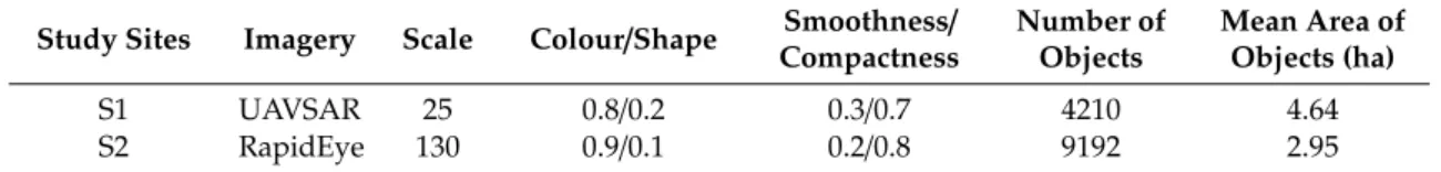
We implemented the multi-resolution segmentation (MRS) algorithm in the eCognition Developer [56]. Three control parameters, namely, scale, colour/shape and smoothness/compactness, were tuned by means of a systematic trial-and-error process. A relatively small value of the scale parameter was set for a small amount of over-segmentation, thus, assuring the homogeneity of the segmented objects. The optimal combinations of image segmentation parameters over the two study sites are summarised in Table2.
Table 2.Parameters used in the multi-resolution segmentation algorithm in the two study sites.
Study Sites Imagery Scale Colour/Shape Smoothness/ Compactness Number of Objects Mean Area of Objects (ha) S1 UAVSAR 25 0.8/0.2 0.3/0.7 4210 4.64 S2 RapidEye 130 0.9/0.1 0.2/0.8 9192 2.95
3.2.2. Model Structure and Parameter Settings
The object-based SVM (OSVM) model involves two major parameters that need to be pre-defined, the penalty parameter (C) and the kernel parameter (γ), each of which has been shown to influence model outputs [57]. The former determines the trade-offbetween model complexity and training error, while the latter controls the shape of the hyperplane. To search for the best parameters for the model, a “grid-search” on C andγwith exponentially growing sequences (i.e., 10-2, 10-1,. . ., 103) using
Remote Sens.2019,11, 2370 10 of 20
five-fold cross-validation was performed [49]. The optimal combination of parameters over both study sites was found to be 1000 and 0.1, by which the OSVM delivered the best classification results.
For the object-based CNN (OCNN) model, a range of pre-defined parameters need to be tuned, including the input window size, the number of layers, as well as the number of convolutional filters. The input window size of the OCNN was determined through cross-validation from a series of window sizes {24×24, 32×32, 40×40, 48×48, 56×56, 64×64}, and 40×40 and 32×32 were found to be the
optimal sizes for S1 and S2, respectively. To balance network complexity and generalization ability, the number of network layers was tuned to six (Figure5) and a 2×2 max pooling layer following
each convolutional layer was used to further generalise the extracted features. The other parameters were designated as follows: the filter size was 3×3 for the convolutional layers (except for the first
layer which was 5×5); the number of filters in each convolutional layer was 32; the learning rate and
the number of epochs were respectively 0.01 and 500 to fully extract high-level features contained in the images. The cross-entropy loss was employed as the objective function. For training the entire network, the mini-batch stochastic gradient descent with a batch size of 20 samples was adopted to minimise the loss function. The CNN was built using Keras library with Tensorflow backend.
Remote Sens. 2019, 11, 2370 10 of 20
The object-based SVM (OSVM) model involves two major parameters that need to be pre-defined, the penalty parameter (C) and the kernel parameter (γ), each of which has been shown to influence model outputs [57]. The former determines the trade-off between model complexity and training error, while the latter controls the shape of the hyperplane. To search for the best parameters for the model, a “grid-search” on C and γ with exponentially growing sequences (i.e., 10-2, 10-1, …, 103) using five-fold cross-validation was performed [49]. The optimal combination of parameters over both study sites was found to be 1000 and 0.1, by which the OSVM delivered the best classification results.
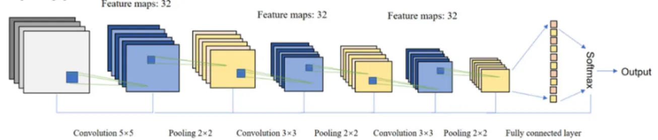
For the object-based CNN (OCNN) model, a range of pre-defined parameters need to be tuned, including the input window size, the number of layers, as well as the number of convolutional filters. The input window size of the OCNN was determined through cross-validation from a series of window sizes {24 × 24, 32 × 32, 40 × 40, 48 × 48, 56 × 56, 64 × 64}, and 40 × 40 and 32 × 32 were found to be the optimal sizes for S1 and S2, respectively. To balance network complexity and generalization ability, the number of network layers was tuned to six (Figure 5) and a 2 × 2 max pooling layer following each convolutional layer was used to further generalise the extracted features. The other parameters were designated as follows: the filter size was 3 × 3 for the convolutional layers (except for the first layer which was 5 × 5); the number of filters in each convolutional layer was 32; the learning rate and the number of epochs were respectively 0.01 and 500 to fully extract high-level features contained in the images. The cross-entropy loss was employed as the objective function. For training the entire network, the mini-batch stochastic gradient descent with a batch size of 20 samples was adopted to minimise the loss function. The CNN was built using Keras library with Tensorflow backend.
Figure 5. The model structure and parameter settings of the CNN network employed in this research.
3.2.3. Pixel-wise Classifiers and Their Parameters
The RBF SVM model was used for traditional pixel-wise SVM classification. The two control parameters (C and γ) were optimised using a “grid-search” approach as mentioned above [49], and the optimal combination of parameters was found to be 100 and 1.
The traditional pixel-wise CNN also requires a pre-defined series of control parameters. The input window size was selected from {16 × 16, 24 × 24, 32 × 32, 40 × 40 and 48 × 48} and 24 × 24 was found to be the optimal patch size at both the S1 and S2 sites. The number of layers was tuned to six and the number of filters at each convolutional layer was set to 32. The size of convolutional filters was 5 × 5 for the first convolutional layer and 3 × 3 for the other layers, the same as for the OCNN. The learning rate and the maximum number of iterations were designated as 0.01 and 500, respectively.
3.3. Decision Fusion Parameters
A rule-based decision fusion approach was performed based on the OCNN’s prediction probability and the classification results of both OSVM and OCNN models. As mentioned above, the parameter of the decision fusion rules was optimised by a grid search approach through cross-validation. The optimal threshold (α) was found to be 0.98 at S1 and 0.91 at S2, respectively.
Figure 5.The model structure and parameter settings of the CNN network employed in this research.
3.2.3. Pixel-wise Classifiers and Their Parameters
The RBF SVM model was used for traditional pixel-wise SVM classification. The two control parameters (C andγ) were optimised using a “grid-search” approach as mentioned above [49], and the optimal combination of parameters was found to be 100 and 1.
The traditional pixel-wise CNN also requires a pre-defined series of control parameters. The input window size was selected from {16×16, 24×24, 32×32, 40×40 and 48×48} and 24×24 was found
to be the optimal patch size at both the S1 and S2 sites. The number of layers was tuned to six and the number of filters at each convolutional layer was set to 32. The size of convolutional filters was 5×5
for the first convolutional layer and 3×3 for the other layers, the same as for the OCNN. The learning
rate and the maximum number of iterations were designated as 0.01 and 500, respectively.
3.3. Decision Fusion Parameters
A rule-based decision fusion approach was performed based on the OCNN’s prediction probability and the classification results of both OSVM and OCNN models. As mentioned above, the parameter of the decision fusion rules was optimised by a grid search approach through cross-validation. The optimal threshold (α) was found to be 0.98 at S1 and 0.91 at S2, respectively.
3.4. Results and Analysis
3.4.1. Classification Maps and Visual Assessment
The classification maps achieved by the OSVM-OCNN were examined at both study sites. We compared the new OSVM-OCNN method with its two sub-models (OSVM and OCNN), as well as the PSVM and PCNN. To provide a clear visualization, Figures6and7illustrate visual inspections of the classification maps using subset images of the two study sites. It is clear that the PSVM achieved
Remote Sens.2019,11, 2370 11 of 20
undesirable results (salt-and-pepper noise), as demonstrated in Figures6and7. Moreover, tomato and pepper, as well as walnut and almond, were frequently misclassified as each other, as shown in Figure6a,c. However, the PCNN has certain advantages over the PSVM in discriminating these crop classes with similar spectral characteristics. For example, as illustrated by Figures6c and7a, walnut and alfalfa were better distinguished from almond and tomato, respectively, in comparison to the PSVM classifications. Additionally, the salt-and-pepper noise was reduced to some extent due to the use of contextual information. The salt-and-pepper noise still existed in the CNN classifications (especially in the UAVSAR-based CNN classification), and the misclassifications between pepper and tomato and walnut and almond were still present, as illustrated in Figures6and7.
3.4. Results and Analysis
3.4.1. Classification Maps and Visual Assessment
The classification maps achieved by the OSVM-OCNN were examined at both study sites. We compared the new OSVM-OCNN method with its two sub-models (OSVM and OCNN), as well as the PSVM and PCNN. To provide a clear visualization, Figures 6 and 7 illustrate visual inspections of the classification maps using subset images of the two study sites. It is clear that the PSVM achieved undesirable results (salt-and-pepper noise), as demonstrated in Figures 6 and 7. Moreover, tomato and pepper, as well as walnut and almond, were frequently misclassified as each other, as shown in Figure 6a,c. However, the PCNN has certain advantages over the PSVM in discriminating these crop classes with similar spectral characteristics. For example, as illustrated by Figure 6c and Figure 7a, walnut and alfalfa were better distinguished from almond and tomato, respectively, in comparison to the PSVM classifications. Additionally, the salt-and-pepper noise was reduced to some extent due to the use of contextual information. The salt-and-pepper noise still existed in the CNN classifications (especially in the UAVSAR-based CNN classification), and the misclassifications between pepper and tomato and walnut and almond were still present, as illustrated in Figures 6 and 7.
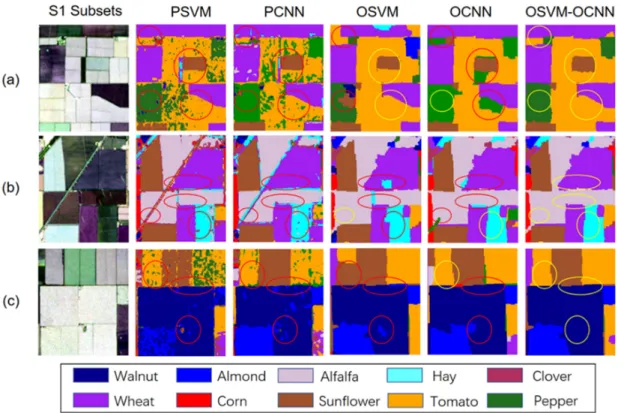
Figure 6. Three representative subsets (a, b and c) from the UAVSAR imagery with the corresponding classification maps; the first column shows the UAVSAR images (bands VV, HV and HH), the following columns illustrate the classification maps achieved by the PSVM, PCNN, OSVM, OCNN, and the proposed OSVM-OCNN, respectively; the regions with correct and incorrect classification results were labelled with yellow and red circles, respectively.
In contrast to the pixel-wise SVM and CNN, the classification maps generated by the object-based SVM and CNN exhibited very smooth visual appearance, and the salt-and-pepper noise was removed, as shown in Figures 6 and 7. The classification of fruit crops (walnut and almond), forage crops (alfalfa and hay) and summer crops (corn, tomato and pepper) was also improved to some extent as shown by the yellow circles in Figures 6 and 7. Specifically, parts of tomato were misclassified by the OCNN, whereas these areas were accurately classified by the OSVM (Figure 6a). In contrast, the OSVM was less accurate than the OCNN when identifying hay and tomato (Figure
Figure 6. Three representative subsets (a–c) from the UAVSAR imagery with the corresponding classification maps; the first column shows the UAVSAR images (bands VV, HV and HH), the following columns illustrate the classification maps achieved by the PSVM, PCNN, OSVM, OCNN, and the proposed OSVM-OCNN, respectively; the regions with correct and incorrect classification results were labelled with yellow and red circles, respectively.
In contrast to the pixel-wise SVM and CNN, the classification maps generated by the object-based SVM and CNN exhibited very smooth visual appearance, and the salt-and-pepper noise was removed, as shown in Figures6and7. The classification of fruit crops (walnut and almond), forage crops (alfalfa and hay) and summer crops (corn, tomato and pepper) was also improved to some extent as shown by the yellow circles in Figures6and7. Specifically, parts of tomato were misclassified by the OCNN, whereas these areas were accurately classified by the OSVM (Figure6a). In contrast, the OSVM was less accurate than the OCNN when identifying hay and tomato (Figure6b,c). Similarly, the OSVM was more accurate than the OCNN in identifying wheat and tomato while the OCNN showed certain advantages over the OSVM in discriminating alfalfa, walnut and cucumber (Figure7).
Remote Sens.2019,11, 2370 12 of 20
Remote Sens. 2019, 11, 2370 12 of 20
6b,c). Similarly, the OSVM was more accurate than the OCNN in identifying wheat and tomato while the OCNN showed certain advantages over the OSVM in discriminating alfalfa, walnut and cucumber (Figure 7).
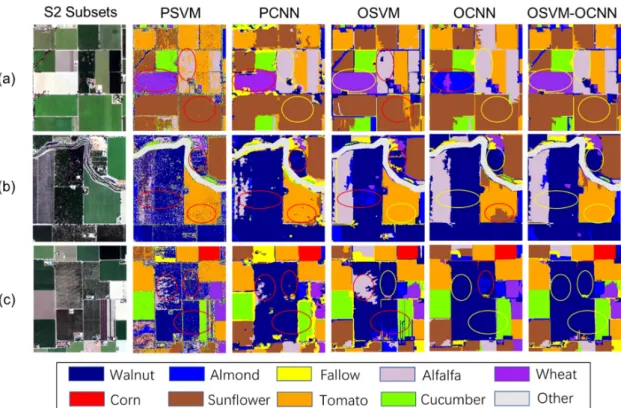
Figure 7. Three representative subsets (a, b and c) from the RapidEye imagery with the corresponding classification maps; the first column shows the RapidEye images (bands Red, Green and Blue), the following columns illustrate the classification maps achieved by the PSVM, PCNN, OSVM, OCNN and the proposed OSVM-OCNN, respectively; the regions with correct and incorrect classification results were labelled with yellow and red circles, respectively.
When checking the classification maps of the OSVM-OCNN, most of the aforementioned misclassifications achieved by OSVM and OCNN were revised while keeping the smoothness of the classifications. For example, the OSVM-OCNN modified the misclassifications of the OSVM for pepper, as shown in Figure 6a, and for sunflower and walnut, as shown by Figure 7, which benefitted from the accurate classification of the OCNN. Moreover, the OSVM-OCNN revised the classification errors of the OCNN for tomato (Figure 6a and Figure 7b) and wheat (Figure 7a). More importantly, some mutual misclassifications between the OSVM and OCNN were effectively resolved. For example, as illustrated in Figure 6b,c, some wheat and walnut patches were misclassified as hay and almond, respectively, in both the OSVM and OCNN classifications; however, they appeared at different places, and nearly all the mislabelled patches were rectified when combining the two classification results using the decision fusion strategy provided in this research.
3.4.2. Classification Accuracy Assessment
In addition to visual assessment, we further investigated the classification accuracy of the proposed OSVM-OCNN and the other benchmark methods, including the PSVM, PCNN, OSVM, and the OCNN over the two study sites. Tables 3 and 4 list the detailed classification accuracy of the methods in both S1 and S2 using the overall accuracy (OA), Kappa coefficient (𝜅) and per-class mapping accuracy. As shown in the tables, the OSVM-OCNN acquired the greatest OA of 90.74% at S1 and 86.63% at S2 with 𝜅 of 0.90 and 0.85, respectively, consistently greater than the OCNN (86.86% and 81.68% OA with 𝜅 of 0.85 and 0.79, respectively) and OSVM (86.42% and 81.39% with
Figure 7. Three representative subsets (a–c) from the RapidEye imagery with the corresponding classification maps; the first column shows the RapidEye images (bands Red, Green and Blue), the following columns illustrate the classification maps achieved by the PSVM, PCNN, OSVM, OCNN and the proposed OSVM-OCNN, respectively; the regions with correct and incorrect classification results were labelled with yellow and red circles, respectively.
When checking the classification maps of the OSVM-OCNN, most of the aforementioned misclassifications achieved by OSVM and OCNN were revised while keeping the smoothness of the classifications. For example, the OSVM-OCNN modified the misclassifications of the OSVM for pepper, as shown in Figure6a, and for sunflower and walnut, as shown by Figure7, which benefitted from the accurate classification of the OCNN. Moreover, the OSVM-OCNN revised the classification errors of the OCNN for tomato (Figures6a and7b) and wheat (Figure7a). More importantly, some mutual misclassifications between the OSVM and OCNN were effectively resolved. For example, as illustrated in Figure6b,c, some wheat and walnut patches were misclassified as hay and almond, respectively, in both the OSVM and OCNN classifications; however, they appeared at different places, and nearly all the mislabelled patches were rectified when combining the two classification results using the decision fusion strategy provided in this research.
3.4.2. Classification Accuracy Assessment
In addition to visual assessment, we further investigated the classification accuracy of the proposed OSVM-OCNN and the other benchmark methods, including the PSVM, PCNN, OSVM, and the OCNN over the two study sites. Tables3and4list the detailed classification accuracy of the methods in both S1 and S2 using the overall accuracy (OA), Kappa coefficient (κ) and per-class mapping accuracy. As shown in the tables, the OSVM-OCNN acquired the greatest OA of 90.74% at S1 and 86.63% at S2 withκof 0.90 and 0.85, respectively, consistently greater than the OCNN (86.86% and 81.68% OA withκof 0.85 and 0.79, respectively) and OSVM (86.42% and 81.39% with correspondingκof 0.85 and 0.79, respectively). The increase in classification accuracy was much more conspicuous when compared to the pixel-wise classifiers, such as the PCNN (81.31% and 79.11% OA withκof 0.79 and 0.76, respectively) and PSVM (72.75% and 70.20% OA with correspondingκof 0.70 and 0.66, respectively). In addition, a McNemar test developed for pair-wise comparison further demonstrated
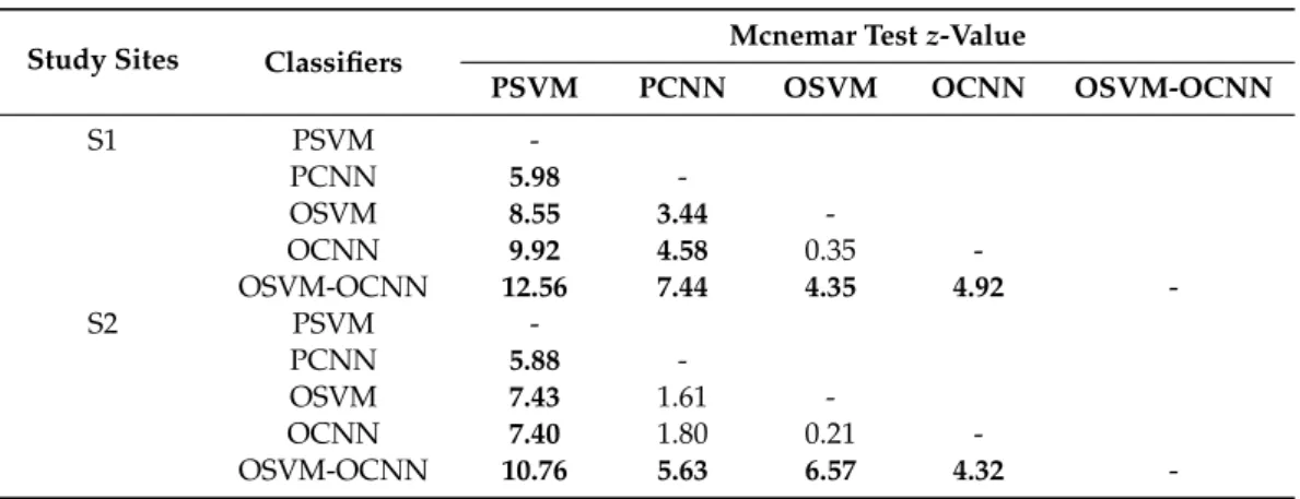
the proposed OSVM-OCNN achieved significantly increased classification accuracy in comparison with the PSVM and PCNN, as well as the OSVM and OCNN, withz-value=12.56, 7.44, 4.35 and 4.92 in S1 andz-value=10.76, 5.63, 6.57 and 4.32 in S2, respectively (Table5). However, there was no significant difference between the OSVM and OCNN classifications over both study sites despite the OAs of the OCNN being slightly higher than those of the OSVM.
Table 3.Overall accuracy as well as per-class accuracy achieved by the PSVM, PCNN, OSVM, OCNN and OSVM-OCNN method with the UAVSAR image in S1; the greatest classification accuracy per row is highlighted in bold font.
Crop Type PSVM PCNN OSVM OCNN OSVM-OCNN
Walnut 80.91 87.85 84.58 91.89 96.33 Almond 76.56 88.60 86.76 91.15 95.65 Alfalfa 72.51 88.35 84.87 88.26 89.96 Hay 62.56 77.94 76.35 89.00 87.37 Clover 71.68 90.83 91.63 91.16 94.17 Winter wheat 70.13 64.68 83.47 80.49 83.26 Corn 83.82 88.00 89.20 95.89 96.39 Sunflower 69.60 80.46 95.51 85.96 93.62 Tomato 74.89 74.89 89.16 81.27 87.55 Pepper 63.16 70.71 80.18 74.40 83.10
Overall accuracy (OA) 72.75 81.31 86.42 86.86 90.74
Kappa coefficient (k) 0.70 0.79 0.85 0.85 0.90
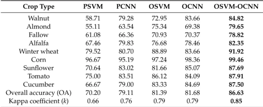
Table 4.Overall accuracy as well as per-class accuracy achieved by the PSVM, PCNN, OSVM, OCNN and OSVM-OCNN method with the RapidEye image in S2; the greatest classification accuracy per row is highlighted in bold font.
Crop Type PSVM PCNN OSVM OCNN OSVM-OCNN
Walnut 58.71 79.28 72.95 83.66 84.82 Almond 55.11 63.54 75.34 69.38 79.65 Fallow 61.08 66.36 70.93 70.37 78.82 Alfalfa 67.46 79.83 76.68 78.46 82.35 Winter wheat 79.52 80.70 88.89 83.66 91.92 Corn 96.67 95.19 97.24 98.36 99.46 Sunflower 70.64 83.02 81.66 85.07 87.69 Tomato 75.00 83.51 86.12 84.09 87.91 Cucumber 66.67 79.00 83.33 84.69 87.50
Overall accuracy (OA) 70.20 79.11 81.39 81.68 86.63
Kappa coefficient (k) 0.66 0.76 0.79 0.79 0.85
The superiority of the OSVM-OCNN method was also checked with class-wise accuracy assessment (Tables3and4). As shown in the tables, the OSVM-OCNN achieved the most accurate class-wise classification for most of the crop types in S1 and all types in S2. The largest increase was up to 8.70% for pepper in S1 and 10.27% for almond in S2, when compared with the OCNN. The accuracy increase was also significant for sunflower (7.66%) and tomato (6.28%) in S1 and fallow (8.45%) and winter wheat (8.26%) in S2. In comparison to the OSVM, most crop classes in S1 and all classes in S2 were classified with greater accuracy with the OSVM-OCNN. Specifically, walnut exhibited the greatest increase in accuracy over both study sites, up to 11.75% at S1 and 11.87% at S2, respectively. As for winter wheat, sunflower and tomato in S1, the accuracy of the OSVM-OCNN was slightly less than that of the OSVM without significant differences. The accuracy increase of the OSVM-OCNN tended to be more obvious in comparison to the PSVM and PCNN. Here, the OSVM-OCNN was constantly superior to the PCNN and PSVM at the class-wise level, with the largest increase up to 18.58% and 24.81% for winter wheat and hay in S1 and 16.11% and 26.11% for almond and walnut in S2, respectively.
Remote Sens.2019,11, 2370 14 of 20
Table 5.McNemar test results for comparing the performance of the five methods over both study sites; bold font indicates that the compared two methods are significantly different at the 95% confidence level.
Study Sites Classifiers Mcnemar Testz-Value
PSVM PCNN OSVM OCNN OSVM-OCNN
S1 PSVM -PCNN 5.98 -OSVM 8.55 3.44 -OCNN 9.92 4.58 0.35 -OSVM-OCNN 12.56 7.44 4.35 4.92 -S2 PSVM -PCNN 5.88 -OSVM 7.43 1.61 -OCNN 7.40 1.80 0.21 -OSVM-OCNN 10.76 5.63 6.57 4.32
-For the four benchmark methods themselves (i.e., the PSVM, PCNN, OSVM and the OCNN), the OCNN achieved the greatest accuracy, followed by the OSVM and PCNN, while the PSVM was the least accurate. In S1, the two object-based methods (OSVM and OCNN) were significantly more accurate than the two pixel-wise methods (PSVM and PCNN), as demonstrated by the McNemar test (Table5). In S2, the accuracies of the OSVM and OCNN were significantly greater than that of the PSVM (z=7.43 and 7.40, respectively), but only slightly (about 2%) greater than that of the PCNN with no significant difference (z=1.61 and 1.80, respectively). Between the same type of classifiers, it was found that the PCNN performed significantly more accurately than the PSVM (z=5.98 and 5.88, respectively), while there was no difference between the OSVM and OCNN (z=0.35 and 0.21, respectively) at both study sites as shown in Table5.
The proposed OSVM-OCNN method and the other benchmark comparators were also validated using additional scenes of UAVSAR and RapidEye imagery at S1 and S2 study sites. The classification accuracy assessment including the overall accuracy (OA) and Kappa coefficient (k) was summarised in Table6. The OA andkof both study sites are in accordance with the previous experimental results, where the hybrid OSVM-OCNN achieves the greatest OA of 70.28% at S1 and 76.44% at S2, consistently larger than the two sub-modules (OSVM and OCNN), the PCNN, and the PSVM (Table6). Such coherency of classification accuracy further demonstrates the generalisability of the proposed method.
Table 6.Classification accuracy comparison amongst PSVM, PCNN, OSVM, OCNN and the proposed OSVM-OCNN method using additional UAVSAR and RapidEye imagery.
Imagery Date Accuracy PSVM PCNN OSVM OCNN OSVM-OCNN
UAVSAR 03/10/2011 OA 57.23% 68.17% 67.37% 68.61% 70.28%
k 0.52 0.65 0.64 0.65 0.67
RapidEye 07/09/2016 OA 52.77% 68.32% 73.56% 72.77% 76.44%
k 0.47 0.64 0.70 0.69 0.73 3.5. Influence of the Decision Fusion Parameter
In this subsection, the contribution of the decision fusion parameter (α) (i.e., the prediction probability of the OCNN model) in combining classification results of the two sub-modules (OSVM and OCNN) is investigated (Figure8). Herein, Figure8a shows the relations between parameterαand the final classification accuracy (through fusion decision) in S1 (dots in orange) and S2 (dots in blue), respectively; whereas Figure8b illustrates the area percentage of the OCNN predictions influenced by αin the fused classification map over the two study sites. From Figure8a, it can be seen that, although there was a difference in accuracy between the two sites resulting from different types of remotely
Remote Sens.2019,11, 2370 15 of 20
sensed images, the general tendencies in overall accuracy influenced byαover S1 and S2 were similar: the accuracy increased continuously until reaching the maximum accuracy (α=0.98 in S1 andα=0.91 in S2), and then tended to decrease with further increases inα. Here,α=0.98 andα=0.91 were found to be the optimal decision fusion parameters in S1 and S2, respectively. From Figure8b, it is clear that whenαwas small, OCNN predictions dominated the fused outputs with little contribution from the OSVM; in contrary, too large a value forαresulted in a rapid decrease in the area percentage of CNN predictions, leading to a sharp decrease in overall accuracy (Figure8a). Whenαapproached initially the optimal value, the CNN predictions with low confidence were gradually replaced by accurate SVM predictions, resulting in a rapid increase in accuracy (Figure8a). The selection of the optimal αvalue, thus, clearly demonstrates the complementary properties between the two sub-modules by the proposed decision fusion strategy.
3.5. Influence of the Decision Fusion Parameter
In this subsection, the contribution of the decision fusion parameter (α) (i.e., the prediction probability of the OCNN model) in combining classification results of the two sub-modules (OSVM and OCNN) is investigated (Figure 8). Herein, Figure 8a shows the relations between parameter α and the final classification accuracy (through fusion decision) in S1 (dots in orange) and S2 (dots in blue), respectively; whereas Figure 8b illustrates the area percentage of the OCNN predictions influenced by α in the fused classification map over the two study sites. From Figure 8a, it can be seen that, although there was a difference in accuracy between the two sites resulting from different types of remotely sensed images, the general tendencies in overall accuracy influenced by α over S1 and S2 were similar: the accuracy increased continuously until reaching the maximum accuracy (α = 0.98 in S1 and α = 0.91 in S2), and then tended to decrease with further increases in α. Here, α = 0.98 and α = 0.91 were found to be the optimal decision fusion parameters in S1 and S2, respectively. From Figure 8b, it is clear that when α was small, OCNN predictions dominated the fused outputs with little contribution from the OSVM; in contrary, too large a value for α resulted in a rapid decrease in the area percentage of CNN predictions, leading to a sharp decrease in overall accuracy (Figure 8a). When α approached initially the optimal value, the CNN predictions with low confidence were gradually replaced by accurate SVM predictions, resulting in a rapid increase in accuracy (Figure 8a). The selection of the optimal α value, thus, clearly demonstrates the complementary properties between the two sub-modules by the proposed decision fusion strategy.
Figure 8. (a) Variation in classification accuracy and (b) area percentage of the CNN predictions in the fused output, plotted against α.
4. Discussion
Accurate classification of FSR remotely sensed images is considered a major challenge within the remote sensing community [57]. Combination of different classifiers is an effective means to solve the complex FSR image classification problem, where single classifiers should be as unique as possible, so as to produce different decision boundaries [38]. However, traditional classifier fusion methods by integrating classifiers at the pixel level are unsuitable for processing FSR imagery, given the potential for large amounts of noise (see the salt-and-pepper noise in the PSVM classifications, Figures 6 and 7).
In this research, a novel method (OSVM-OCNN) was proposed for the first time by fusing the outputs of the object-based SVM (OSVM) and CNN (OCNN) at the object level for crop classification from FSR images. The OSVM determines the decision boundaries among classes based completely on the low-level within-object information (e.g., spectral, polarimetric, texture; [24]). In such a manner, the OSVM can identify the objects with salient spectral properties (i.e., light regions on the Figure 3b), but has difficulty handling those objects with similar within-object information (e.g., the
Figure 8.(a) Variation in classification accuracy and (b) area percentage of the CNN predictions in the fused output, plotted againstα.
4. Discussion
Accurate classification of FSR remotely sensed images is considered a major challenge within the remote sensing community [57]. Combination of different classifiers is an effective means to solve the complex FSR image classification problem, where single classifiers should be as unique as possible, so as to produce different decision boundaries [38]. However, traditional classifier fusion methods by integrating classifiers at the pixel level are unsuitable for processing FSR imagery, given the potential for large amounts of noise (see the salt-and-pepper noise in the PSVM classifications, Figures6and7).
In this research, a novel method (OSVM-OCNN) was proposed for the first time by fusing the outputs of the object-based SVM (OSVM) and CNN (OCNN) at the object level for crop classification from FSR images. The OSVM determines the decision boundaries among classes based completely on the low-level within-object information (e.g., spectral, polarimetric, texture; [24]). In such a manner, the OSVM can identify the objects with salient spectral properties (i.e., light regions on the Figure3b), but has difficulty handling those objects with similar within-object information (e.g., the misclassifications between two types of forage crops (alfalfa and hay), Figure6b). This is due mainly to the unavailability of high-level between-object information. In fact, for a large crop parcel, it is normally segmented into several small objects due to the heavy spectral and spatial variations. If only the within-object information is utilised, some of the segmented objects might be misclassified. However, if the between-object (contextual) information is also taken into account, sufficiently representative information can be achieved for the objects, thus markedly increasing the chance of correctly identifying those objects. The OCNN extracts hierarchical features from images via an input window using multiple convolution and pooling operations [24]; thus, both low-level and high-level features are incorporated into the classification process. However, with a fixed input window, the OCNN is incapable of