Methodological Development and Advances for Joint Modelling of Longitudinal and Time-To-Event Data

(1)

This version was downloaded from Northumbria Research Link: http://nrl.northumbria.ac.uk/39722/

Northumbria University has developed Northumbria Research Link (NRL) to enable users to access the University’s research output. Copyright © and moral rights for items on NRL are retained by the individual author(s) and/or other copyright owners. Single copies of full items can be reproduced, displayed or performed, and given to third parties in any format or medium for personal research or study, educational, or not-for-profit purposes without prior permission or charge, provided the authors, title and full bibliographic details are given, as well as a hyperlink and/or URL to the original metadata page. The content must not be changed in any way. Full items must not be sold commercially in any format or medium without formal permission of the copyright holder. The full policy is available online: http://nrl.northumbria.ac.uk/policies.html

(2)

ADVANCES FOR JOINT MODELLING OF

LONGITUDINAL AND TIME-TO-EVENT DATA

G BUYRUKOGLU

PhD

(3)

ADVANCES FOR JOINT MODELLING OF

LONGITUDINAL AND TIME-TO-EVENT DATA

GONCA BUYRUKOGLU

A thesis submitted in partial fulfilment of the

requirements of the University of Northumbria at

Newcastle for the degree of Doctor of Philosophy

Research undertaken in the Department of

Mathematics, Physics and Electrical Engineering

(4)

Univariate joint modelling of longitudinal and time-to-event data is a simul-taneous analysis of repeated measurements taken from the same individual over time, until an event of interest occurs. This method has attracted increas-ing interest in the literature over the last two decades. In practice, clinical studies are increasingly likely to record more complex data structures (such as multilevel longitudinal data or multiple longitudinal profiles, along with event time data) than single longitudinal and event time data. This thesis develops a methodology and software for both multilevel and multivariate joint

mod-els accounting for complex longitudinal data, by focusing on random effects

selection models, where information from the longitudinal trajectories is used to inform the event-time process. The research also assesses the power of the score test, which is a prognostic tool to investigate the association between sub-models, before fitting potentially complex and computationally intensive joint models under a variety of scenarios. The methodology is tested via simula-tion studies, and implemented in various real datasets. The results show that the advanced joint models can provide unbiased estimators when the model is specified correctly such that it utilizes all available data, and that the score test is a powerful tool when the longitudinal profile is highly associated with the event time data. Based on preliminary findings using discrimination measures, the advanced joint models should be preferred in case of complex longitudinal data in order to improve the predictive capability of the model.

(5)

(6)

I declare that the work contained in this thesis has not been submitted for any other award and that it is all my own work. I also confirm that this work fully acknowledges opinions, ideas and contributions from the work of others. Any ethical clearance for the research presented in this thesis (Research project RE-EE-14-150330-5519570105a64) has been approved. Approval has been sought and granted by the Faculty Ethics Committee on 30 March 2015.

I declare that the Word Count of this Thesis is 37460 words.

Name: Gonca Buyrukoglu

Signature:

(7)

I would like to express my sincere gratitude to my supervisors Dr. Pete Philip-son and Dr. Nan Lin for the continuous support they provided during my PhD study and related research, and for their patience, motivation, and immense knowledge. Their guidance helped me during the entire research process and writing of this thesis. I could not have imagined having better supervisors and mentors for my PhD study.

I would like to express my sincere gratitude to the Republic of Turkey’s Min-istry of National Education for the funding provided for my research studentship and the warm support provided throughout.

Very special thanks go to my husband, Selim, my daughter, Feyza and my son, Yusuf for their love, support, understanding and the many sacrifices they made

throughout the period of my study. Also, I offer my grateful thanks to my

(8)

Abstract i

Dedication ii

Declaration iii

Acknowledgements iv

1 Introduction 3

1.1 Longitudinal data analysis . . . 4

1.2 Survival data analysis . . . 6

1.3 Joint modelling of longitudinal and survival data . . . 8

1.3.1 Links between missing data mechanisms and joint mod-elling . . . 11

1.4 Challenges . . . 11

1.5 Case studies . . . 12

1.5.1 SLS data . . . 13

1.5.2 Liver cirrhosis trial . . . 15

1.5.3 ADNI data . . . 16

1.6 Aim and objectives . . . 18

1.7 Layout of the thesis . . . 20

2 Joint modelling of longitudinal and time-to-event data 21 2.1 Introduction . . . 21

2.2 Linear mixed-effects model . . . 24

2.3 Survival analysis . . . 25

(9)

2.3.2 Models for survival analysis . . . 27

2.3.3 The Cox proportional hazards model . . . 28

2.4 The standard joint model . . . 31

2.4.1 The longitudinal submodel . . . 32

2.4.2 The survival submodel . . . 32

2.5 Choice of latent process . . . 33

2.6 Maximum likelihood estimation . . . 35

2.7 Simulation studies . . . 36

2.7.1 Simulation study I . . . 37

2.7.2 Simulation study II . . . 44

2.8 Analysis of liver cirrhosis data . . . 49

2.9 Discussion . . . 51

3 Development of the Methodology for Joint Modelling of Time-To-Event and Multilevel Longitudinal Data with An Application to the SLS Data 55 3.1 Introduction . . . 55

3.2 Model and notation . . . 58

3.3 The linear random effects model and the likelihood function . . 61

3.3.1 The random intercept and slope model at subject and centre-levels . . . 61 3.3.2 Likelihood function . . . 62 3.4 Estimation method . . . 63 3.5 Simulation studies . . . 66 3.5.1 Simulation study I . . . 66 3.5.2 Simulation study II . . . 71

3.6 Application: the scleroderma lung study . . . 74

4 A score test for univariate joint models 80 4.1 Introduction . . . 80

4.2 Model and notation . . . 82

(10)

4.4.1 Comparison of power of the score test based on two vari-ance structures . . . 98

5 A score test for complex joint models 105 5.1 Introduction . . . 105

5.2 Models and notation . . . 106

5.3 Score test for association . . . 108

5.3.1 Score test for the separate association parameter . . . 108

5.3.2 Score test for association of multivariate joint model . . . 109

5.3.3 Score test for the cluster level association . . . 111

5.4.1 Simulation study I - investigation of the power of the sep-arate effect score test . . . 113

5.4.2 Simulation study II - investigation of the power of the multivariate score test . . . 119

5.4.3 Simulation study III - investigation of the power of the multilevel score test . . . 122

6 Joint Modelling of Time-To-Event and Multivariate Longitudinal Data: An Application to the ADNI Dataset 130 6.1 Introduction . . . 130

6.2 Patient population and study design . . . 132

6.3 Measures . . . 133

6.3.1 Neuropsychological assessment . . . 133

6.3.2 Functional and behavioural assessment . . . 134

6.3.3 Neuroimaging . . . 134

(11)

6.5 Predictive survival probabilities and prospective accuracy for the

multivariate joint models . . . 138

6.5.1 Predictive survival probabilities . . . 138

6.5.2 Discrimination for multivariate longitudinal biomarkers 139 6.6 Results . . . 141

6.6.1 Results of the multivariate joint models . . . 142

6.6.2 Results of the univariate joint models . . . 145

6.6.3 Results for score test . . . 146

6.6.4 Results of discrimination for multivariate longitudinal biomark-ers and predictive accuracy . . . 151

7 Assessing robustness of univariate joint models for longitudinal and time-to-event data 158 7.1 Introduction . . . 158 7.2 Method . . . 161 7.3 Simulation study . . . 161 7.3.1 Study design . . . 161 7.3.2 Simulation results . . . 163 7.4 Discussion . . . 170

8 Conclusions and Further Work 172 8.1 Introduction . . . 172

8.2 Summary of the thesis . . . 172

8.3 Limitations and future work . . . 176

8.4 Conclusion . . . 178

Appendices 179 A Appendix 180 A.1 Calculation of the score and information . . . 180

A.2 Gauss-Hermite Quadrature . . . 182

A.3 Score Test results for Model D with separate association . . . 183

(12)

1.1 Frequencies of the event types for the SLS data . . . 14

2.1 Some common lifetime distributions . . . 27

2.2 Simulation results based on 1000 sample size and 500

simula-tions, with a 70% event rate, Scenario I. . . 41

2.3 Simulation results based on 1000 sample size and 500

simula-tions, with a 25% event rate, Scenario II. . . 42

2.4 Joint model parameter estimation results under misspecified

ran-dom effects models. Complicated data with simple model fit.

MSE: mean square error, CP: coverage probability. . . 47

2.5 Joint model parameter estimation results under misspecified

ran-dom effects models. Simple data with complicated model fit.

MSE: mean square error, CP: coverage probability. . . 48

2.6 Log likelihoods for liver cirrhosis trial based on separate analysis 51

2.7 Parameter estimates (Est) and standard errors (SE) of liver

cir-rhosis trial, with three different latent association structure:

ran-dom intercept model (Model I), ranran-dom intercept and slope model

(Model II), and random quadratic model (Model III). . . 52

3.1 Simulation results for the multi-level joint model (based on a

sample size ofn= 1000 and 1000 simulations) . . . 69

3.2 Simulation results of two scenarios (Scenario A: mean of event rate is 72%, and Scenario B: mean of event rate is 24%). Standard

errors are obtained via bootstrap samples. . . 70

(13)

3.4 The SLS data results for two differentW1(t) models: a random in-tercept model at both levels with proportional association (Model

C), and a random intercept model at subject-level (Model A). . . 76

4.1 Selection of the chosen parameters to achieve the relevant event

rate, and to adapt the simulations to the scenarios for Model A. . 90

4.2 The power of the score test expressed as a percentage for Model A, with a representative small sample of the simulation results for each scenario. Longitudinal and survival data are linked

through the association parameterγ, with independence atγ = 0. 90

rate, and to adapt the simulations to the scenarios for Model B. . 91

4.4 The power of the score test expressed as a percentage for Model B, with a representative small sample of the simulation results for each scenario. Longitudinal and survival data are linked

rate, and to adapt the simulations to the scenarios for Model C. . 92

4.6 The power of the score test expressed as a percentage for Model C, with a representative small sample of the simulation results for each scenario. Longitudinal and survival data are linked

rate, and to adapt the simulations to the scenarios for Model D. . 94

4.8 The power of the score test expressed as a percentage for Model D, with a representative small sample of the simulation results for each scenario. Longitudinal and survival data are linked

4.9 Score statistics and p-values of the SLS data using martingale and bootstrap variance . . . 100

(14)

4.10 The SLS data results for two different W1(t) models: a random intercept model at subject-level (Model A), and a random inter-cept and slope model at subject-level with proportional associa-tion (Model B) . . . 101 5.1 Indicative powers of the score test (in percent) for Model B with

a representative small sample of the simulation results for each scenario. Longitudinal and survival data are linked through the

association parameterγ, with independence atγ= 0. . . 116

5.2 Indication of power of the score test in percentage for Model C with a representative small sample of the simulation results for each scenario. Longitudinal and survival data are linked through

the association parameterγ, with independence atγ= 0. . . 118

5.3 Indication of power of the score test in percentage for Model D with a representative small sample of the simulation results for Scenario III. Longitudinal and survival data are linked through

the association parameterγ, with independence atγ= 0. . . 119

5.4 Indication of power of the score test in percentage for Models E and F with a representative small sample of the simulation results. Longitudinal and survival data are linked through the

5.5 Indication of power of the score test in percentage for Models C and D with a representative small sample of the simulation results. Longitudinal and survival data are linked through the

5.6 Score test statistics and p-values of the sls data under the null hypothesis using martingale and bootstrap variance having sep-arate association between the two components. . . 127 5.7 SLS data results for random-intercept-and-slope with separate

association (Model B) . . . 127 6.1 The correlation matrix of the six biomarkers of the ADNI data. . 137

(15)

6.2 Baseline characteristics of ADNI-I participants with MCI. The data corresponding to women and APOE4 are given as number of participants (percentage), while the others are given as mean (SD). . . 142 6.3 Indication of the power of the score test in percentage for a

ran-dom intercept and slope model with a representative small sam-ple of the simulation results for Scenario I and II: Scenario I, 70% event rate; Scenario II, 25% event rate. Longitudinal and

sur-vival data are linked through the association parameter γ, with

independence atγ= 0. . . 147

6.4 The MVJM results for prediction of risk of AD progression for the first 10 models. . . 148 6.5 The MVJM results for prediction of risk of AD progression for

the second 10 models. . . 149 6.6 The univariate JM results for prediction of risk of AD progression.150 7.1 The parameters chosen for the implementation of scenarios in

the simulation studies - mean and variance of the number of re-peated measurements per subject with their SDs, and event rates experienced across 100 simulations. . . 163 7.2 Simulation results of bias MSEs and coverage probabilities of

joint model parameter estimates under Scenario I. . . 167 7.3 Simulation results of bias MSEs and coverage probabilities of

joint model parameter estimates under Scenario II. . . 168 7.4 Simulation results of bias MSEs and coverage probabilities of

joint model parameter estimates under Scenario III. . . 169 A.1 The powers of the score test, event rates and association

(16)

1.1 Profile plots of FVC% for CYC (0) group vs. placebo (1) group.

Red line shows (smoothed) mean index . . . 14

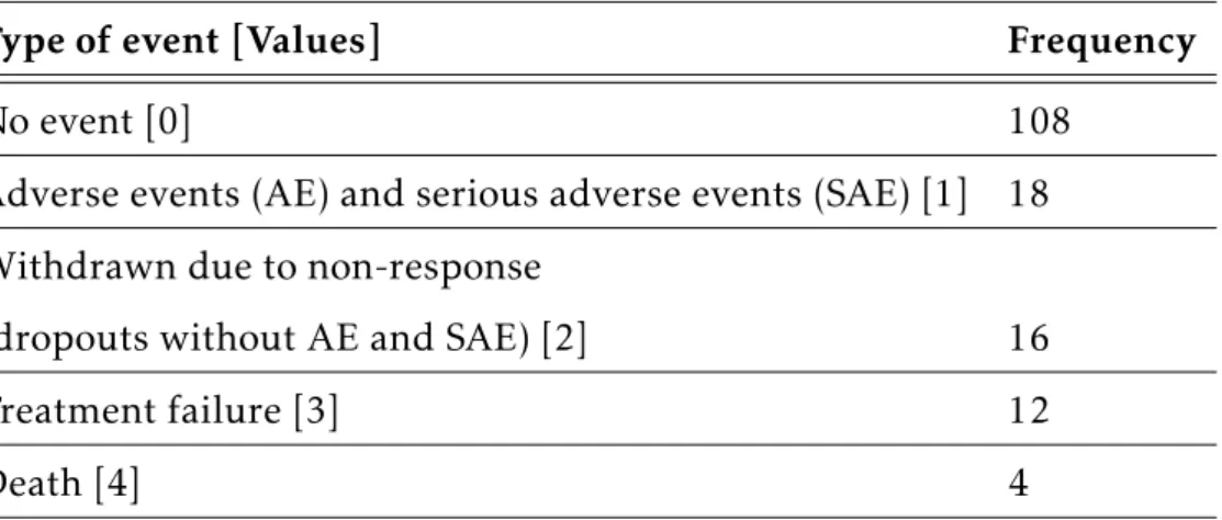
1.2 Patient survival with 95% CI bands on the SLS study . . . 15

1.3 Survival probability of liver cirrhosis trial per treatment group

with associated 95% CI bands. . . 16

1.4 Longitudinal profiles of prothrombin index per treatment group

for patients who were censored/died. . . 17

1.5 Survival probability of ADNI data with associated 95% CI bands. 18

2.1 Left panel - Kaplan-Meier estimate of the survival function for the liver cirrhosis data. Right panel - Nelson-Aalen estimate of

the cumulative hazard function for the liver cirrhosis data. . . . 29

2.2 Longitudinal trajectories of prothrombin index of each

individ-ual censored (left panel) or died (right panel). . . 50

3.1 Joint plot of the SLS data . . . 77

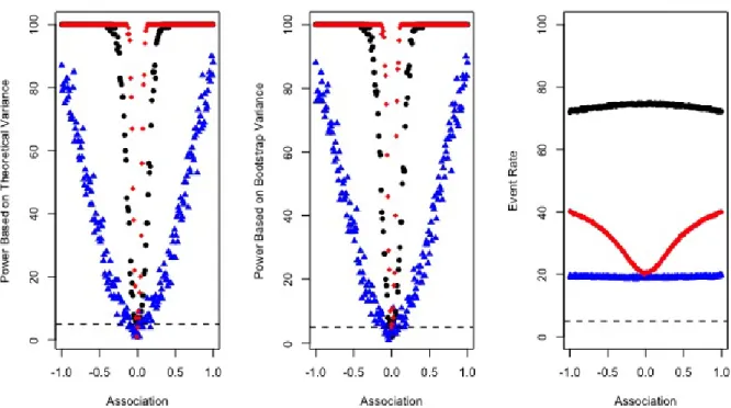
4.1 Power and event rate for Model A: • _{(black) represent a high}

event rate (Scenario I);N_{(blue) a low event rate (Scenario II); and}

q(red) mimicked SLS data (Scenario III). Theoretical variance

(left panel), bootstrap variance (mid panel), event rate (right panel)

(17)

4.2 Power and event rate for Model B: • _{(black) represents a high}

event rate (Scenario I); N _{(blue) a low event rate (Scenario II);}

and q(red) mimicked SLS data (Scenario III). Theoretical

vari-ance (left panel), bootstrap varivari-ance (mid panel), and event rate

(right panel) are also shown. . . 91

4.3 Power and event rate for Model C: • _{(black) represent a high}

event rate (Scenario I);N_{(blue) a low event rate (Scenario II); and}

q(red) mimicked SLS data (Scenario III). Theoretical variance

are also shown. . . 93

4.4 Power and event rate for Model D: • _{(black) represents a high}

event rate (Scenario I); N _{(blue) a low event rate (Scenario II);}

q(red) mimicked the SLS data (Scenario III). Theoretical variance

are also shown. . . 95

4.5 Difference in the score test power with various latent associations

(on the x-axis) for Scenario I and Models A-D (clockwise from

top-left). . . 99

(on the x-axis) for Scenario II and Models A-D (clockwise from

top-left). . . 99

(on the x-axis) for Scenario III and Models A-D (clockwise from top-left). . . 104 5.1 Power based on theoretical variance (left panel), power based

on bootstrap variance (mid panel) and event rate (right panel)

vs two different association parameters for Model B. The upper

plots represent Scenario I, the middle plots represent Scenario II, the lower plots represent Scenario III. . . 114

(18)

5.2 Power based on theoretical variance (left panel), power based on bootstrap variance (mid panel) and event rate (right panel)

vs two different association parameters for Model C. The upper

plots represent Scenario I, the middle plots represent Scenario II, the lower plots represent Scenario III. . . 117 5.3 Powers of the multivariate score test and event rates of the

sim-ulated dataset for Models E and F. . . 123

5.4 Power of multilevel score test and event rate:• _{(black) for}

ran-dom intercept and slope model at both level;N_{(red) for random}

intercept model at both level. Theoretical variance (left panel), bootstrap variance (mid panel), event rate (right panel). . . 124 6.1 The longitudinal trajectories of each participants who are

cen-sored or not. The upper plot shows trajectories of ADAS-Cog 13, while the lower plot shows trajectories of Cog 11. ADAS-Cog refers to Alzhemier’s Disease Assessment Scale-ADAS-Cognitive Subscale test. . . 143 6.2 The longitudinal trajectories of each participants who are

cen-sored or not. The upper plot shows trajectories of CDR-SB, while the lower plot shows trajectories of FDG-PET. CDR-SB refers to Clinical Dementia Rating Sum of Boxes; whereas FDG-PET refers to the sum of mean glucose metabolism uptake in regions of an-gular, temporal, and posterior cingulate. . . 144 6.3 The conditional time-to-event distribution for a new subject from

the last observation time, given their longitudinal history data. . 152 6.4 The conditional expected longitudinal values for Patient 1300

from the last observation time, given their longitudinal history data. . . 152 6.5 Boxplots of AUCs for all possible models including three

biomark-ers: ADAS-Cog 13, FAQ, and MidTemp. The order is univariate models for ADAS-Cog 13, FAQ, and MidTemp; bivariate models for pairs ADAS-Cog 13 - FAQ, ADAS-Cog 13 - MidTemp, and FAQ - MidTemp; and lastly, the trivariate model. . . 154

(19)

7.1 Indicative histograms based on a simulated dataset indicating the number of repeated measurement times per subjects for Sce-narios I, II and III. . . 162

(20)

Introduction

The joint modelling of longitudinal and survival data has become a highly-active field of research over the past twenty years. The original methodology

for a univariate random effects joint model has been developed by Wulfsohn

and Tsiatis (1997) and extended by Henderson et al. (2000), and has become known as the standard joint model. Recent developments have considered joint models for multivariate longitudinal data and a single survival data (Lin et al., 2002), as well as for a single longitudinal and multivariate survival data (Williamson et al., 2008). The standard joint model considers a linear mixed

effects submodel for the longitudinal data and a Cox-based submodel for the

time-to-event data, and links these submodels through shared random effects.

The various random effects’ structure can change the nature of the association.

Historically, joint models were applied to data arising from clinical trials. More recently, trials across multiple centres and countries have been conducted to combat serious diseases. Furthermore, on a larger scale, there has been consid-erable interest in utilising electronic healthcare databases. Such databases can link repeated measurements with the event’s history record. Each of these sce-narios points to the need for joint modelling approaches that are considered to

be the most efficient way to capture available information from two (or more)

data sources, giving rise to longitudinal data and survival data. This chapter describes the fundamentals of longitudinal and survival data analysis.

(21)

1.1

Longitudinal data analysis

Longitudinal data is very common in practice, featuring in numerous appli-cations such as epidemiology, clinical trials, economics, industry and biology. In longitudinal studies, individuals are followed over time and measurements are taken from the same individual repeatedly. The main goal of a longitu-dinal study is to characterize the change in response over time, and find out

the factors that affect the change. Responses between subjects may be

inde-pendent; however, repeated measurements taken from the same individual are very likely to be correlated. This causes the violation of the independence as-sumption, which is one of the fundamental assumptions in traditional statisti-cal methodology. This dependency amongst measurements within individuals makes longitudinal data analysis a specialist statistical research area.

The mixed effects modelling framework (also known as the random effects

models) is an important data analytic class for longitudinal data analysis. These models consider the relationship between serial observations on the same unit. While the general covariance structure is hardly applicable to these kinds of

models, two-stage random effects models can be applied easily. In these

mod-els, the explanatory variables are obtained by regression parameters as in the

traditional regression, where the random effects parameters vary across

indi-viduals and capture any subject-specific deviations. The subject-specific

ran-dom effects parameters are specified at the second stage. A general family of

such models is discussed in the seminal paper of Laird and Ware (1982), which

incorporates both growth models and random effects models.

Further development of the statistical methodology for longitudinal data anal-ysis continued over the following three decades. For instance, Diggle (1988) proposed a linear model for longitudinal data by accounting for the serial cor-relation structure within the same unit, and the utilization of the variogram of residuals to determine the suitable correlation structure of repeated mea-surements. On the other hand, Taylor et al. (1994) developed a plausible and

(22)

parsimonious model to describe the stochastic process underlying the patterns of longitudinal data, which enables one to understand if the subjects keep their trajectories. In addition, Jennrich and Schluchter (1986) presented a parameter estimation approach for unbalanced and incomplete repeated measurements using the maximum likelihood (ML) method along with some numerical algo-rithms such as Newton-Raphson methods and the expectation maximization (EM) algorithm, which was originally discussed by Dempster et al. (1977). In this context, Lindstrom and Bates (1988) improved the implementation of the algorithm presented by Jennrich and Schluchter (1986), and sped up the con-vergence at each iteration. Longitudinal data is discussed in more details in numerous literature sources, such as the books authored by Verbeke (1997), Diggle (2002), Fitzmaurice et al. (2008) and Fitzmaurice et al. (2012).

The assumption of the most well-known linear mixed effects model for a

con-tinuous response is that the random effects and the within-subject errors have

normal distribution. This assumption makes the model sensitive to outliers,

and these outliers can be problematic for mixed effects models, as they are

likely to be seen in the random effects and make them difficult to detect in

practice. As a solution, Pinheiro et al. (2001) proposed random effects models

having a repeated measurement multivariate t distribution to be able to cope with this problematic issue.

Researchers use many different kinds of statistical software programmes to

im-plement longitudinal data analysis. However, the R programming language,

which is an open-source software programme, is preferred in this work, and is used throughout this thesis (R Core Team, 2017). There are two packages

available to implement longitudinal data analysis inR, namely nlme(Pinheiro

et al., 2017) andlme4(Bates et al., 2015). Whilst these packages are able to fit

the Laird-Ware model,nlme can also fit random effects models with a

station-ary Gaussian process (SGP). Due to the superiority of thenlmepackage and the

chance of the possible extension to the incorporation of the SGP in joint model,

(23)

regarding all data simulation, analysis of the simulated data and real data can

be found athttps://github.com/goncabuyrukoglu.

1.2

Survival data analysis

Survival data (also known as time-to-event data) are the main interest of many fields, such as epidemiology, biology and medicine, in which the primary in-terest lies in the time it takes from a given baseline for an event of inin-terest to occur, and the identification of any factors related to this event. An example of

this would be studying the effect of a treatment on the time-to-dementia (event)

since diagnosis of mild cognitive impairment. The analysis of such data is de-scribed as time-to-event analysis or survival analysis. This section provides a brief introduction to the survival data analysis and an overview of the current literature.

The probability of experiencing an event of interest, the rate at which the event occurs, and how the rate changes among groups are some of the outcomes of in-terest from time-to-event analysis. A distinguishable characteristic of survival data is that, not all participants experience the event within the follow-up time. This leads to censoring problems. There are three types of censoring problems, namely right censoring, left censoring and interval censoring.

Right censoring happens when the event of interest does not appear within the specified time frame. It is the most common censoring type. For exam-ple, in a cohort study, patients who have been diagnosed with breast cancer are followed, and two groups of treatment are investigated in terms of the time-to-death, and are compared to each other. While, some patients may live up to 30 years after treatment, it is generally not feasible to continue to study after a specified point due to resources constraints, such as finance or time. If a pa-tient has not experienced the event within the follow-up time, this is described as administrative censoring and considered as non-informative censoring. If a patient moves from one place to another or withdraws from the study for

(24)

rea-sons related to the outcome, then this is called informative censoring.

Left censoring occurs when the event of interest happens before a patient starts to be observed or before the outcome is verified. It generally occurs when the event of interest is the relapse of a disease. The data cannot be left censored when the event is death. If a patient already has cancer before the follow-up, it can be an example of left censored data.

Interval censoring occurs when the event of interest occurs within an interval and covers the other two scenarios (i.e. is a combination of left and right cen-soring). It occurs when the event time is between two time points. Following the previous example, if the relapse does not occur in the first visit of the clinic, and is instead found in the following visit, then the actual time to relapse is be-tween the first visit and second visit.

Event times are necessarily positive and are typically right skewed data. Con-sidering the censoring, right skewness of data, and having the interest mostly on hazard and survival functions makes survival data analysis complicated, requiring the development of bespoke statistical methods and software pro-grammes, as in the case of longitudinal data analysis.

Survival data was first addressed by Kaplan and Meier (1958), in which sur-vival data analysis methods compared sursur-vival curves amongst groups. A re-markable development in medical and statistical research was published by Sir David Cox in 1972 (Cox, 1972), which is one of the most important research publications in this field, with over 46,000 citations (Google Scholar, January 2018) since its publication. The method presented in the research is a semi parametric approach with the incorporation of explanatory variables, and has become known as the Cox proportional hazards model. The Cox model es-timates the parameters via the partial likelihood method by generalizing the ideas of conditional and marginal likelihood (Cox, 1975), and does not as-sume any particular form of baseline hazard function. It is one of the main

(25)

approaches and is often used as the default choice in the analysis of survival data. The other types of approaches (which assume exponential or Weibull dis-tribution) for the survival times are fully parametric approaches, such as that of Collett (2015). The original Cox model deals with only constant covariates through time. It was then extended to incorporate time-dependent covariates through a counting process approach (Andersen and Gill, 1982), based on the Aalen model BAS¸AR (2017). Vaida and Xu (2000) proposed a general

propor-tional hazards model with random effects (known as the frailty model), and

Yamaguchi et al. (2002) extended it to allow for centre variation in the

treat-ment effects, as well as baseline risks.

Oakes (2013) published a useful overview with some key ideas and models in survival analysis. However, the interested reader is referred to Kleinbaum (1998) as a starting self-learning resource on survival analysis, while for ad-vanced methods, the reader may find it useful to be referred to the extended survival data analysis textbooks written by Kalbfleisch and Prentice (2011), Lawless (2011), Lee and Wang (2003) and Hosmer et al. (2008). Furthermore, Andersen et al. (1993) is an interesting resource for survival data analysis with

counting processes. In addition, the survival package (Therneau, 2015) is

available to implement survival data analysis, and contains some auxiliary func-tions such as the comparisons of survival curves, along with fitting of a range of models.

1.3

Joint modelling of longitudinal and survival data

In medical studies, longitudinal outcomes are often intrinsically collected with event time data, even if this is not ostensibly the focus of the study, as it is sometimes a natural requirement of the longitudinal data. However, these out-comes are analysed separately, despite the obvious potential that the two types of outcomes are associated. When this potential association is to be explored, a more complex method to analyse the two data types needs to be considered. This brings us to a popular, novel and rapidly growing research area over the

(26)

past twenty years, namely the field of joint modelling of longitudinal and sur-vival data (also known as simultaneous analysis of the two types of outcomes).

The most well-known approach, also known as the standard joint modelling of longitudinal and time-to-event data, was developed by Wulfsohn and Tsiatis

(1997), combining the linear mixed effect model with a proportional hazards

model through shared random effects with maximum likelihood, implemented

via the EM algorithm, which is used for parameters estimation. This method characterises the association between the two outcomes. A joint model allows much greater insight into both outcomes, with reduction of bias, making an optimal use of the available data with an attempt to disentangle the underly-ing association in an interpretable manner (Lawrence Gould et al., 2015). An early study to accommodate longitudinal data as a time dependent covariate into survival models was carried out by Andersen and Gill (1982). However, the drawback of this study is the assumption of perfectly measured covariates and their availability at each time point. In practice, it is nearly impossible for this assumption to hold in any moderate sized study. Real life observations are prone to measurement errors, they are taken possibly intermittently and of un-equally spaced time points for the repeated measurements, and possibly subject to censoring event times. A further study to improve this method was proposed by Tsiatis et al. (1995), and is referred to as a two-stage analysis of longitudinal and time-to-event data. In the first stage, the method models the longitudinal data using a repeated measurements random components model (in a separate analysis), and in the second stage, the parameters in the survival model are estimated by considering the observed values as a time dependent covariate in the Cox model. Nevertheless, Sweeting and Thompson (2011) stated that a two-stage model can severely underestimate the association between the un-derlying longitudinal value and event hazard. Simultaneous analysis of the two outcomes handles the aforementioned drawbacks of the two-stage approach.

Berzuini and Larizza (1996) investigated the simultaneous modelling of lon-gitudinal and survival data from the Bayesian perspective, and Faucett and

(27)

Thomas (1996) used MCMC techniques of Gibbs sampling to estimate the joint posterior distribution of the unknown parameters. These studies combine the

random effects for longitudinal data and the proportional hazards model for

event times data. Henderson et al. (2000) extended the joint modelling frame-work with a flexible parametrisation of association structure between the two outcomes, incorporated into special cases of the model, and described a Monte Carlo EM estimation procedure considering the two components to be linked through a latent stationary Gaussian process. While Henderson et al. (2000) used maximum likelihood estimation via the EM algorithm using antithetic pairs, Guo and Carlin (2004) investigated flexible parametrisation with a Bayesian paradigm.

As the joint modelling is an active and popular research field, there are now many published studies that have extended this by developing either the lon-gitudinal or survival side of the modelling. Sousa (2011) reviewed the joint

modelling of longitudinal and survival data in detail, and stated that different

factorisations of the joint distribution can bring about different model

inter-pretations such as pattern-mixture and selection models, which are explained in detail in the following chapter. The interested reader may be referred to read the review papers published by McCrink et al. (2013), Lawrence Gould et al. (2015) and Sousa (2011) for extensive information on joint models. For

further reading, the book-length material of Elashoffet al. (2016) and

Rizopou-los (2012), which are solely dedicated to joint models, can be useful. There

are four packages for joint models in theRprogramming language, namely JM

(Rizopoulos, 2010),joineR(Philipson et al., 2017) for ML estimation,JMbayes

(Rizopoulos, 2016) for Bayesian approaches, andjoineRML(Hickey et al., 2017)

for joint models of multivariate longitudinal data and time-to-event outcomes.

Thestjmpackage is also available to fit shared parameter joint models inStata

(28)

1.3.1

Links between missing data mechanisms and joint

mod-elling

Missing data is a common occurence and a major challenge in longitudinal studies. Longitudinal studies are designed to collect data on every single sub-ject in sample; however it is often not the case encountered in practice. Some data are not complete due to a variety of reasons and this brings about the term ’missing data’ (Little and Rubin, 2014; Molenberghs and Kenward, 2007; Ibrahim and Molenberghs, 2009). Rubin (1976) classified the missing data mechanisms into three categories:

• MCAR (missing completely at random): Missingness depends neither on observed nor unobserved measurements.

• MAR (missing at random): Missingness depends on observed measure-ments, but not on unobserved measurements.

• MNAR (missing not at random): Missingness depends on unobserved measurements conditional on observed measurements.

Joint modelling is closely linked with dropouts in that dropout time can be considered as survival outcome. A clear distinction is that, from missing data perspective, the dropout is typically inferred from an individual’s failing to be present at a scheduled follow-up time due to some reasons and considered as discrete time outcome, whilst time-to-event of interest is recorded or censored at the study end-time from joint modelling perspective. Thus, there is an asso-ciation between the dropout and the underlying longitudinal trajectories and this can be considered missing not a random (MNAR), which can potentially

affect the conclusions in case of ignoring the missing data in longitudinal

anal-ysis.

1.4

Challenges

As with any emerging research area, joint modelling has some statistical and methodological challenges which need to be addressed. Rizopoulos (2012)

(29)

claims that sample size and power calculations, as well as the general design of joint modelling have still a long way to go to unify the research methodology to the same levels seen in classic regression models.

The standard closed-form sample size calculations cannot be applied to the joint models. Numerical simulation is the only viable tool due to the

complex-ity of joint models. Multiple visit times of subjects, as well as different number

of visiting times and causes of dropouts need to be considered carefully. This research starts with considering the standard joint modelling assumptions of a

single event of interest and a linear mixed effect model for longitudinal

mea-surements, and extend the methodology by relaxing the assumptions.

Consid-ering more complex random effect structure leads to further technical issues in

joint modelling. The approach of this study is a hybrid of theory and simula-tion.

It is worth noting that several important situations have yet to receive the requi-site attention in joint modelling literature. For example, the treatment of asyn-chronous longitudinal profiles, multi-level data structures, sample size and power calculations, residuals and model fitting, dynamic prediction, model se-lection, handling of large multivariate datasets are all yet to be addressed. We will address some of these issues in this dissertation. Some of these problems can be dealt with simulation studies and comparisons with existing research studies.

1.5

Case studies

In this section, three datasets that contain different characteristics that the rest

of the thesis seeks to explore are introduced, namely a multicentre dataset (al-beit with a small sample), a multivariate longitudinal dataset with over thirty biomarkers, and a dataset with atypically long follow-up.

(30)

1.5.1

SLS data

The Scleroderma Lung Study, a 13-centre double-blind, randomized, placebo-controlled trial sponsored by the National Institutes of Health, was designed

to evaluate the effectiveness and safety of one-year oral intake of

cyclophos-phamide (CYC) in patients with active, symptomatic scleroderma-related in-terstitial lung disease (Tashkin et al., 2006). Data was available from 158 pa-tients, equally distributed into two treatment groups, namely CYC and placebo,

and followed-up for two years. The study included four different types of

events. There were 4 deaths, 12 treatment failures, 18 adverse events (AE) or serious adverse events (SAE), and 16 participants were withdrawn from the study without AE or SAE. The rest of the patients experienced no events. The event types and their frequencies are indicated in Table 1.1. The primary out-comes of this study are repeated measurements of the FVC (forced vital capac-ity, % predicted) and death/failure times. The dataset was used as an

appli-cation in the textbook of joint modelling written by Elashoffet al. (2016), and

is publicly available after registering athttps://faculty.biostat.ucla.edu/

gangli/jm-book-data, and was downloaded from the aforementioned website on December 15, 2016.

Having multiple centres makes this dataset a good application while investi-gating a multilevel joint model in Chapter 3. The dataset has tied event times, and such ties were broken by subtracting a tiny random value from each tied survival time as suggested by Borucka (2014). Ties in survival data is explained further in Section 2.3.3. In this work, some criteria were set for this dataset. Throughout this thesis, event values [1], [3] and [4] are pooled as having the event, and event values [0] and [2] as having no event, to create a new event indicator, yielding 34 events. Furthermore, 21 measurements taken after hav-ing the event from the seven patients were discarded. Five patients who had missing maximum fibrosis were also discarded. Lastly, 17 patients who did not complete the treatment in the first six months were discarded. In total, 22 patients who did not comply with the criteria (eight of whom had the event)

(31)

Type of event [Values] Frequency

No event [0] 108

Adverse events (AE) and serious adverse events (SAE) [1] 18

Withdrawn due to non-response

(dropouts without AE and SAE) [2] 16

Treatment failure [3] 12

Death [4] 4

Table 1.1: Frequencies of the event types for the SLS data

were discarded. Thus, 136 patients out of 158 were analysed, 26 of whom had the event, and 110 of whom did not have event in the final dataset. Hence,

the event rate of this study is 19.1%. Figure 1.1 shows a plot of the profile

Figure 1.1: Profile plots of FVC% for CYC (0) group vs. placebo (1) group. Red line shows (smoothed) mean index

of FVC% stratified by treatment group. There is a large variation in baseline FVC% suggesting individual heterogeneity. Most patients showed a small vari-ation in FVC% over time, however, there were a few patients with larger or smaller measurements. The bold red line indicates the mean profile of FVC%.

(32)

er-Figure 1.2: Patient survival with 95% CI bands on the SLS study

ence. Figure 1.2 shows the Kaplan-Meier survival curves. As can be seen, there

is little difference between treatment groups in survival during the follow up

time, and the placebo arm seems to be a slightly better treatment choice.

1.5.2

Liver cirrhosis trial

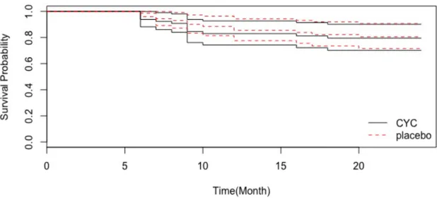
A study investigating the effect of prednisone treatment in patients with liver

cirrhosis is another motivating dataset used throughout this thesis. This study was originally described by Andersen et al. (1993), and an application using prothrombin index as a surrogate biomarker for overall health was made by Henderson et al. (2002). Data is available for 488 patients with 40% censor-ing rate. Furthermore, 251 patients were randomly allocated at diagnosis to prednisone treatment, and 237 patients were randomised to placebo only. The patients were followed until death or the end of the study. In total, 292 patients died during the study. The study lasted 13 years, which is atypically long for a longitudinal study. The primary interests are the prothrombin index, mea-sured repeatedly throughout the study and treatment. This dataset is a stan-dard joint modelling dataset, with exception of the long follow-up time. In the

(33)

Figure 1.3: Survival probability of liver cirrhosis trial per treatment group with associated 95% CI bands.

The curves then diverge, which indicates a possible improved prognosis in the treatment arm (see Figure 1.3). The curves subsequently come together again around nine years into the study.

Figure 1.4 shows some exploration of the observed data, by plotting the longi-tudinal profile of the prothrombin index for each patient who took the placebo (left panel) or prednisone (right panel) treatment. As can be seen, the plot does

not show much difference between the two treatments. The data is publicly

available from theJMpackage inR(Rizopoulos, 2010).

1.5.3

ADNI data

The Alzheimer’s Disease Neuroimaging Initiative (ADNI) study is a longitudi-nal multisite observatiolongitudi-nal study of elderly individuals with normal cognition, mild cognitive impairment (MCI), or Alzheimer’s disease (AD) (Mueller et al., 2005b,a), jointly funded by the National Institute of Health (NIH). The study is designed to assess the performance of magnetic resonance imaging (MRI), (18F)-fludeoyglucose positron emission tomography (FDG PET), urine, serum,

(34)

Figure 1.4: Longitudinal profiles of prothrombin index per treatment group for patients who were censored/died.

and cerebrospinal fluid (CSF) biomarkers, as well as various clinical and neu-rocognitive measures in terms of investigation into the progression of AD in the three groups of elderly individuals (Jack et al., 2008). More detailed infor-mation regarding the study’s procedures and inclusion and exclusion criteria is

available athttp://www.adni-info.org. The data used in this thesis is

pub-licly available after registering on the aforementioned website, and was

down-loaded fromhttp://ida.loni.ucla.eduon October 24, 2017.

The dataset presented here includes 388 patients with MCI at baseline hav-ing at least one follow-up visit, and havhav-ing the protocol from which subject originated is ”ADNI-I”. The criteria for MCI defined by Petersen et al. (1999) and used by Li et al. (2017) are the same as those adopted in this thesis: a memory complaint where objective memory loss is measured by education ad-justed scores on the Wechsler Memory Scale Logical Memory II, a Folstein Mini Mental State Examination Score (MMSE) of 24-30, a Clinical Dementia Rating (CDR) equal to 0.5, absence of significant levels of impairment in functional, behavioural and neuroimaging domains, and essentially preserved activities of their routine. All subjects were given a consent form at the beginning of the

(35)

study, and the study had ethical approval from the local institutional review board at all sites that participated in the study. Having multiple longitudinal biomarkers makes this dataset a unique application for this thesis along with the investigation of multivariate joint modelling in Chapter 6.

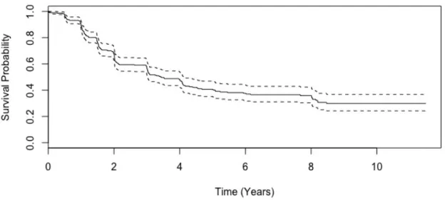
The event of the study considered throughout this thesis is conversion to AD from MCI. There were 205 events recorded for the 388 patients, resulting in an event rate of 52.8%. This study has 33 longitudinal clinical and imaging mea-sures, and is a rich, multivariate dataset. Figure 1.5 depicts the Kaplan-Meier survival curves of the ADNI-I study with the confidence intervals. Information about the baseline characteristics of the ADNI-I subjects with MCI are given in Chapter 6.

Figure 1.5: Survival probability of ADNI data with associated 95% CI bands.

1.6

Aim and objectives

The aim of this research is to extend the current statistical methodology design and incorporate multi-level models and multivariate joint models in order to improve the predictive ability of inference in joint modelling frameworks.

(36)

This aim begets the following objectives:

1. To extend the joint modelling framework to allow for multiple levels (such as the hospital or clinic where a patient was treated or a family

effect), and to explore the consequences of ignoring the centre level effect

when it is actually needed. An application of this is to use the SLS data discussed in the previous section, with rigorous simulation studies used to demonstrate the properties of the multilevel model.

2. To assess the power of the score test for association between biomarker values and survival time, both in the context of the classic Wulfsohn and Tsiatis (1997) joint model and extensions relevant to this work, namely joint models with multilevel latent associations, where in each case, asso-ciation is via a single parameter (i.e. the univariate score test). Simulation studies are utilised to verify findings.

3. To develop an assessment of the power of a multivariate score test for as-sociation between longitudinal biomarkers and survival time when

sepa-rate associations are considered for each random effect, to test whether a

fit of joint models with multilevel random effect structure is needed, and

to assess which biomarker is required to fit in the case of having multiple biomarkers. Simulation studies are performed for a range of scenarios to indicate how powerful the score test is under these situations.

4. To demonstrate how joint modelling can be used to maximise the infor-mation obtained from multiple, correlated longitudinal measurements, in order to improve the predictive ability of multivariate joint models over the univariate joint model and what gain can be made in moving from a univariate joint model to multivariate joint model and investigate the dy-namic nature of the longitudinal profiles for a new patient. A particular application involves ADNI data, as introduced in the previous section.

5. To assess the sensitivity and robustness of the joint models with diff

er-ent sample sizes. Simulation studies are conducted to demonstrate the

(37)

6. To assess the performance of univariate joint models of longitudinal and survival data over a separate analysis of these two components, and to investigate the consequences of fitting misspecified joint models to data

that is generated under three different latent association structures.

Sim-ulation studies with various scenarios and latent association structures are drawn upon to verify findings, and fitting joint models are utilised for the liver cirrhosis data, introduced earlier.

7. To critically appraise all findings, suggest avenues for future research, and conclude on the achievements and challenges of the research appro-priately.

1.7

Layout of the thesis

The thesis is organised as follows. Chapter 2 introduces the joint modelling of longitudinal and time-to-event data, assesses the performance of this technique when compared to the separate analysis of each component, and examines the

impact on misspecified random effects structure in this framework. Chapter

3 develops multilevel joint models that account for centre level effect as well

as individual effects, and investigates the consequences of fitting a joint model

with individual level random effects when the centre level effect is ignored.

Chapter 4 introduces the score test for association between the longitudinal and survival data, and performs simulation studies under various scenarios. Chapter 5 extends the score test for association between these two components with various situations, i.e. univariate joint model in conjunction with a sepa-rate association, multilevel joint model, and multivariate joint model. Chapter 6 introduces the joint modelling of multivariate longitudinal and survival data as well as prospective accuracy and dynamic features of londitudinal biomark-ers, while Chapters 7 presents an assessment of the robustness of the univariate joint model. Finally, Chapter 8 concludes the thesis and provides recommen-dations for future work.

(38)

Joint modelling of longitudinal and

time-to-event data

2.1

Introduction

Although repeated measurements and survival time data are often collected in tandem (e.g. the Alzheimer’s Disease Assessment Scale-Cognitive (ADAS-Cog), and time until the conversion of MCI to AD for the ADNI study explained in Section 6.3 in detail (Li et al., 2017)), they are often analysed separately due

to the lack of availability of suitable software before the emergence of the JM

package inR(Rizopoulos, 2010), and lack of penetration of joint modelling into

other disciplines. A more complex approach involves a requirement to analyse

these two kinds of associated measurements in a more efficient way. This leads

to the joint modelling of longitudinal and time-to-event data, which has seen an explosion of interest in the past twenty years. The aim of joint modelling is to investigate and exploit any potential association between longitudinal mea-surements and time-to-event data. Joint modelling reduces bias and makes the

analysis more efficient by using the available data in an optimum way (Asar

et al., 2015). A common approach involves a combination of linear mixed effect

models and Cox proportional hazards model for the longitudinal and survival

submodels, which can then be linked through the shared random effects.

Tsi-atis and Davidian (2004) illustrated the association between longitudinal and time-to-event data, and gave one of the most common examples used in joint

(39)

modelling literature. In this example, HIV studies, CD4 count cells are mea-sured repeatedly over time as measures immunologic and virologic status, and patients are also followed-up until they contract AIDS or die.

The primary focus for inference on joint modelling may depend on the appli-cation of interest. There are typically three objectives for joint modelling:

1. Inference about the repeated measurements with possible non-ignorable dropout; or

2. The distribution of time-to-event of interest conditional on time-varying longitudinal outcome; or

3. The joint relationship between the longitudinal outcomes and time-to-event process.

For example, Henderson et al. (2000) analysed the PANSS score with the con-sideration to be important, with equal interest in both longitudinal and event time data, third objective.

In joint modelling, full likelihood methods to estimate the parameters from

the joint distribution of the two outcomes can differ depending on the

factori-sation of the joint distribution of the components (Sousa, 2011; McCrink et al., 2013). Bayes’ rule is applied for the factorisation of the joint distribution. The

two different factorisations of the joint distribution require different modelling

strategies in terms of inference of the model. They are referred to as pattern-mixture models and selection models (Little and Rubin, 2014; Little, 1993). If

Y denotes longitudinal outcomes, and T denotes the survival outcomes, the

joint distribution of these two outcomes can be formulated as:

Pattern-mixture models: [Y , T] = [T][Y|_T_] _(2.1)

Selection models: [Y , T] = [Y][T|_Y_] _(2.2)

Although the joint distribution of these two models are the same, they have

different interpretations. The nature of the statistical problem can affect the

(40)

primary interest is the longitudinal outcomes of different patterns of drop-out, which can also have the association between event times. If the inference is on the event times parameters, selection models are used to estimate the model parameters. Simple, yet detailed explanations on these models are provided by

Sousa (2011) and McCrink et al. (2013). Furthermore, Little (2008) and Elashoff

et al. (2016) explain these models in Chapter 4 in detail.

The natural extension of these models is the incorporation of random effects,

which makes the previous models known as random pattern-mixture models and random selection models. The marginal longitudinal models include

in-dividual random effects, which are unobserved in real problems in the former

model, while the marginal distribution of event times are included in the latter model. The models are expressed as: (Sousa, 2011):

Random pattern-mixture models: [Y , T , U] = [U][T|_U_][Y|_T_] _(2.3)

Random selection models: [Y , T , U] = [U][Y|_U_][T|_Y_] _(2.4)

whereU denotes the random effects.

Another different class of joint models is defined by Diggle (1998) as random

ef-fects models. The assumption of this model is that both longitudinal outcomes

and event times are dependent on the individual unobserved random effects,

with a further assumption of conditional independence between repeated

mea-surements and event times, given the random effects. The model is defined as:

Random effects models: [Y , T , U] = [U][Y|_U₁_][T|_U₂_] _(2.5)

whereU = (U1, U2). In these models, the two processes are independent,

con-ditional on the random effects, and the association between these outcomes is

determined by the correlation structure betweenU1 andU2.

The third objective is the primary focus for inference, as the primary

inter-est of this thesis is random effects models. Hence, a detailed explanation of the

statistical methods is first provided for the linear mixed-effects model, survival

(41)

an application of the liver cirrhosis data. Lastly, this chapter is concluded with a brief discussion.

2.2

Linear mixed-e

ff

ects model

In longitudinal studies, serial observations on the same units are taken. A suit-able analysis for such data needs to take this potential dependence within

indi-viduals into account. The linear mixed-effects model (LMEM) is a very effective

and widely used method to deal with unbalanced longitudinal data structures,

which have different number of observations for each subject taken at

poten-tially different times (Laird and Ware, 1982). The LMEM includes three parts,

namely fixed effects, random effects and random errors. The underlying idea of

the LMEM is that regression coefficients may vary randomly from one subject

to another. For instance, different subjects may have different intercepts and

slopes.

Notationally, the LMEM can be outlined as follows. LetYij denote thejth

mea-surements of the ith subject taken at a pre-specified time point of tij. There

are mi measurements taken for the ith subject. That is, j = 1,2, . . . , mi and

i = 1,2, . . . , n, where n is the number of subjects. The model formulation can

then be expressed as follows:

Yij=x1i(t0ij)β1+W1i(tij) +εij, i = 1, . . . , n (2.6)

W1i(tij) =D(tij)

0

Ui, Ui∼N(0,Σ), εij∼N(0, σε2)

whereW1i(tij) is a latent process incorporating random effects,Uis andεijs are

assumed to be mutually independent, β₁ is a p-vector of fixed-effects coeffi

-cients, x₁_i(t_ij)ismi-vector of covariates for individual i, Σ is aq×q

positive-definite variance-covariance matrix, andD(tij) is a vector of explanatory

vari-ables for individuali. To borrow from Crowder (2017), ”To be poetic,x₁_i(t0_ij)

is an immutable constant of the Universe,W1i(tij) is a lasting characteristic of

(42)

The advantages of mixed models include the possibility to estimate parame-ters describing the response changes in the population of interest as well as the ability to predict the changes in the subject response trajectories over time. The overall variability is partitioned between subjects and random errors. Further-more, inference at the subject level is one of the main reasons for using mixed models in the joint modelling of longitudinal data analysis and time-to-event analysis.

2.3

Survival analysis

Survival data are of particular interest in a variety of applied fields such as medicine and biology, where occurrence of certain events times or time to death from the onset of a disease are of particular interest. There are four fundamen-tal functions in a time-to-event analysis, namely the cumulative distribution

function,F(t), the survival function,S(t), the hazard function,h(t), and the

cu-mulative hazard function, H(t). Mathematically, they are intrinsically related

to each other. LetT denote the time to occurrence of an event of interest, and

suppose T has a probability distribution with underlying probability density

function,f(t). One can then express the following:

• The cumulative distribution function: F(t) =P(T ≤_{t) =}

Z t

0

f(u)du (2.7)

• The survival function:

S(t) =P(T > t) = 1−_F(t), _t≥₀ _(2.8)

dS(t)

(43)

• The hazard function: h(t) = lim ∆t→0 P[(t≤_{T < t}₊_∆t)|_T ≥_t] ∆t = lim ∆t→0 1 ∆t P(t≤_{T < t}₊_∆t) P(T ≥_t) = lim ∆t→₀ 1 ∆t P(T < t+∆t)−_P_(T ≤_t) S(t) = lim ∆t→₀ 1 S(t) F(t+∆t)−_F(t) ∆t = F0(t) S(t) h(t) =f(t) S(t) (2.9)

• The cumulative hazard function:

H(t) = Z t 0 h(u)du = Z t 0 f(u) S(u)du= Z t 0 F0(u) S(u)du=− Z t 0 S0(u) S(u)du=−ln[S(t)] H(t) =−_ln_S(t) S(t) = exp(−_H(t)) _(2.10)

The survival and the hazard functions are the most useful functions in terms of explaining risk. The survival function gives the probability of experiencing the event of interest within a specified time frame, while the hazard function gives the rate of experiencing the event per year.

2.3.1

Parametric survival analysis

In survival analysis, using a parametric model can help to gain a greater insight into the observed data, as a result of its flexibility and the fact that it is better for standard errors of parameters. These models, while not considered explicitly here, will be subsequently used to illustrate concepts. They are usually based on the hazard or the log-hazard function, where the hazard can either increase or decrease with time. The assumptions that was made about the shape of the hazard function can specify the time-to-event. There are some parametric dis-tributions in the hazard functions such as exponential, Weibull or Gompertz. The hazard, survival and density functions of these distributions are given in

(44)

Functions h(t) S(t) f(t)

Exponential Distribution λ exp(−_λt) _λ_exp(−_λt)

Weibull Distribution λγtγ−1 exp(−_λtγ₎ _λγtγ−1_exp(−_λtγ₎

Gompertz Distribution λexp(γt) exp{−_λγ−1_(eγt−₁₎} _λ_exp{_γt−_λγ−1_(eγt−₁₎}

Table 2.1: Some common lifetime distributions

The simplest assumption that one can make about the shape of the hazard function is having a constant hazard rate over time, which assumes that the survival times follow an exponential distribution. The Weibull distribution is a more flexible choice for the hazard function, where the hazard rate increases or decreases monotonically. Another parametric distribution is the Gompertz distribution, which is more likely to be used in mortality data. In such a distri-bution, the hazard rate increases or decreases exponentially.

2.3.2

Models for survival analysis

To motivate ideas, the estimation of the survival function of the Kaplan-Meier estimator will be explained, as well as the cumulative hazard function of the Nelson-Aalen estimator. The Cox proportional hazards model will then be dis-cussed.

Kaplan-Meier (KM) estimator

Proposed by Kaplan and Meier (1958), the KM estimator is the most well-known method for comparing survival functions for a small number of groups. It is a non-parametric method that does not require any assumption under-lying the distribution of the failure times. To introduce this estimator, let t1 < t2 < · · · < tk denote the observed event times in a sample of n subjects, and note that some subjects may be censored. The survival function of the KM estimator is defined by:

ˆ SKM(t) = Y ti≤t      1 −di ri       (2.11)

(45)

whereri is the number of subjects at-risk at time ti,di is the number of events

at timeti. The variance of the above survival function can be calculated using

Greenwood‘s formula. V ar( ˆSKM(t)) = ˆSKM(t) 2X ti≤t       di ri(di−ri)       (2.12)

Nelson-Aalen (NA) estimator

Originally suggested by Nelson (1972) and studied by Aalen (1978), the NA es-timator is used to estimate the cumulative number of expected events in a given time. It is an alternative approach to the KM estimator and can be thought of as a non-parametric method to estimate the cumulative hazard function. The NA cumulative hazard rate estimator is given by:

ˆ HN A(t) = X ti≤t di ri (2.13) the survival function based on the NA estimator, using the relation (2.10), can be calculated as: ˆ SN A(t) = exp n −_Hˆ_{N A}_(t)o₌Y ti≤t exp       di ri       (2.14)

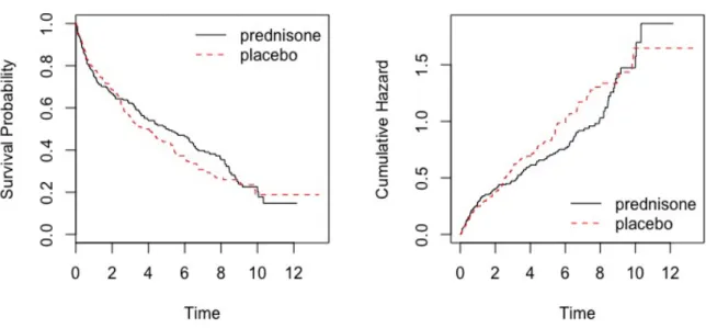
These two estimators of the survival function are asymptotically equivalent. The performance of the NA estimator is slightly superior to that of the KM estimator. However, the KM estimator performs better in terms of decreasing failure rates, while the NA estimator provides better results for increasing fail-ure rates (Colosimo et al., 2002). An illustration of the KM estimator of the survival function and the NA estimator of the cumulative hazard function for the liver cirrhosis data is depicted in Figure 2.1. The survival curves in the left panel of Figure 2.1 show that less than 20% of patients survive 10 years after entry. The prednisone-treated patients have slightly better prognosis than those who were given placebo between around 2 and 10 years into the study.

2.3.3

The Cox proportional hazards model

Time-to-event analysis investigates the relationship of the time-to-event distri-bution to one or more, possibly time-varying, covariates. Usually, specification

(46)

Figure 2.1: Left panel - Kaplan-Meier estimate of the survival function for the liver cirrhosis data. Right panel - Nelson-Aalen estimate of the cumulative hazard function for the liver cirrhosis data.

of a linear-like model is adopted for the log-hazard. For example, a parametric model based on the exponential distribution can be expressed as:

loghi(t) =α+x2iβ2 (2.15)

or equivalently,

hi(t) = exp{α+x2iβ2} (2.16)

wherehi(t) shows the hazard rate for theith subject at time t,x2i is the

covari-ates vector (they do not change over time in this case), β₂ are the associated

regression coefficients that need to be estimated, and α represents a kind of

log-baseline hazard, since loghi(t) =αwhen allx2i elements are zero. It can be

said that equation (2.15) is a linear model for the log-hazard or equation (2.16) is a multiplicative model for the hazard.

In contrast, in the Cox model, the baseline hazard function α(t) = logh0(t) is

unspecified. Equation (2.15) is then written as:

(47)

or equivalently,

hi(t) =h0(t) exp{x2iβ2}

=h0(t) exp(x2iβ2) (2.18)

whereh0(t) = exp{α(t)}.

The Cox model is a semi-parametric model. Whilst it does not require any

assumption about the shape of the baseline hazard, h0(t), it requires some

re-strictive assumptions, one of which concerns tied events (i.e. events with

ex-actly the same time). While h0(t) can take any form of baseline hazard, the

covariates enter the model linearly. The key assumption of equation (2.18) is

that covariate effects remain constant over the follow-up time. Cases with tied

event times never happen if time was measured in a perfectly continuous scale. However, in practice, time is generally measured in a discrete manner, which is more likely to exist in tied event times. Throughout this thesis (as in the SLS data), the ties in survival data are broken by subtracting a small random value from each tied survival time to prevent the violation of this assumption

(Borucka, 2014). This simple method provides results that do not differ from

the exact results to a great extent.

Now, consider two individuals,i andi∗. The hazard ratio is:

hi(t) hi∗(t)= h0(t) exp(x2iβ2) h0(t) exp(x2i∗β2) = exp(x₂_i−x₂_i∗)β 2 (2.19)

which is independent of timet. Since (2.19) is independent of the hazard, the

Cox model is a proportional hazards (PH) model.

Cox (1972) derived a partial likelihood function for the ith subject for a PH

model, which can be expressed as follows: Li(β2) =    