Selective deep convolutional neural network for low cost distorted image classification

Digital Object Identifier 10.1109/ACCESS.2019.2939781

Selective Deep Convolutional Neural Network for

Low Cost Distorted Image Classification

MINHO HA , (Student Member, IEEE), YOUNGHOON BYUN , (Student Member, IEEE), JEONGHUN KIM , JAECHEOL LEE , YOUNGJOO LEE , (Member, IEEE),

AND SUNGGU LEE , (Member, IEEE)

Department of Electrical Engineering, Pohang University of Science and Technology, Pohang 37673, South Korea Corresponding author: Sunggu Lee ([email protected])

This work was supported by Samsung Electronics and Samsung Research Funding & Incubation Center of Samsung Electronics under Project Number SRFC-TB1703-07.

ABSTRACT Neural networks trained using images with a certain type of distortion should be better at classifying test images with the same type of distortion than generally-trained neural networks, given other factors being equal. Based on this observation, an ensemble of convolutional neural networks (CNNs) trained with different types and degrees of distortions is used. However, instead of simply classifying test images of unknown distortion types with the entire ensemble of CNNs, an extra tiny CNN is specifically trained to distinguish between the different types and degrees of distortions. Then, only the dedicated CNN for that specific type and degree of distortion, as determined by the tiny CNN, is activated and used to classify a possibly distorted test image. This proposed architecture, referred to as aselective deep convolutional neural network (DCNN), is implemented and found to result in high accuracy with low hardware costs. Detailed simulations with realistic image distortion scenarios using three popular datasets show that memory, MAC operations, and energy savings of up to 93.68%, 93.61%, and 91.92%, respectively, can be achieved with almost no reduction in image classification accuracy. The proposed selective DCNN scores up to 2.18× higher than the state-of-the-art DCNN model when evaluated using NetScore, a comprehensive metric that considers both CNN performance and hardware cost. In addition, it is shown that even higher hardware cost reduction can be achieved when selective DCNN is combined with previously proposed model compression techniques. Finally, experiments conducted with extended types and degrees of image distortion show that selective DCNN is highly scalable.

INDEX TERMS Artificial intelligence, convolutional neural network, image classification, image distortion. I. INTRODUCTION

Deep convolutional neural networks (DCNNs) perform well in image classification tasks [1]–[5]. However, as increas-ingly deeper and larger DCNNs are used in order to get better accuracies, the number of weight parameters and the number of multiply-and-accumulate (MAC) operations required also increase accordingly [6]. This situation is problematic when researchers attempt to apply these latest DCNN approaches in cloud edge computing nodes or mobile systems, both of which will not have extremely high computing capability [7]. The main motivation for the research described in this paper is the perceived room for improvement in the currently avail-able methods for distorted image classification in limited

The associate editor coordinating the review of this manuscript and approving it for publication was Tae Hyoung Kim.

power budget and/or computing resource environments, such as would be the case for a mobile embedded device with-out cloud computing support (due to network disruption, response-time, or total computing constraints).

In recent years, researchers have shown that even severely distorted images (with high noise levels, blurring, low-light, etc.) can be classified with high accuracy [8]–[12]. However, the methods proposed in these studies use very large and deep CNN structures, and are thus all solutions with high hardware and energy usage requirements.

Image classification methods have also been devised for mobile computing environments. MobileNets [6] and its later varsion, MobileNetV2 [13], are low hardware cost image classification methods specifically designed for mobile com-puting environments, but which do not consider their use for distorted image classification. More recently, a Fast Fourier

Transform(FFT)-based method [14] has been proposed for distorted image classification with low computing overhead. However, this method assumes that the distortion type and degree of the input image can easily classified based on 2D frequency characteristics of the input image, which may not always be case. Also, Wong [15] has proposed a compre-hensive metric, termedNetScore, that considers not only the performance of a DCNN but also its hardware cost [15].

To enable distorted image classification with low hardware costs, this paper proposes a two stage CNN architecture in which only one dedicated CNN needs to be active at any given time and a separate tiny CNN is used to select the dedicated CNN to use. The tiny CNN architecture produces close to perfect classification of distortion type/degree and, as the name implies, is much smaller than a dedicated CNN designed to classify images with distortions of a specific type and degree. Additionally, in order to further reduce hardware costs, the unimportant weights can be pruned without an excessive degradation in classification accuracy.

Experiments were conducted to compare the proposed selective DCNN with the best comparable previous state-of-the-art multi-level distorted image classification DCNN architectures [12], [14] using the SVHN [16], CIFAR-100 [17], and Caltech-256 [18] datasets. Experimental results showed that the proposed selective DCNN achieved sig-nificantly higher NetScores [15], which is a comprehen-sive metric that considers both hardware costs and DCNN accuracy, for all datasets [16]–[18] than two comparison target DCNNs [12], [14]. It was also found that there is a huge reduction in energy usage when using selective DCNN. To summarize, selective DCNN required significantly lower hardware costs than the previous state-of-the-art DCNN architectures while at the same time maintaining relatively high image classification accuracy.

This paper is organized as follows. Section II reviews the related work and introduces motivation for this work. SectionIIIexplains the proposed method. SectionIVpresents evaluation results. Finally, SectionVconcludes the paper.

II. RELATED WORK

There have been several studies on distorted image classi-fication using a CNN. Dodge and Karam [8] analyzed how various distortion classes and levels affect various DCNN models. Zhouet al.[9] also analyzed the effect of different set of distortions on DCNN performance. These studies [8], [9] analyzed the impact of image distortion on DCNN, but did not propose specific solutions to improve accuracy. Dia-mond et al. [10] proposed a denoising/deblurring method that improves the accuracy but requires additional complex computations.

Byun et al. [14] proposed a DCNN architecture, called DCS-CNN in this paper from now on, for classifying dis-tortion types using an FFT-based disdis-tortion classifier and a method for effectively scaling the number of channels of an DCNN according to the distortion classification result. Fig.1 shows concept of DCS-CNN. However, classifying distortion

FIGURE 1. The concept of DCS-CNN [14] targeting (a) Gaussian noise level 2 case and (b) Gaussian blur level 1 case (C: clean, B: Gaussian blur, N: Gaussian noise).

types using an FFT is only effective with specific types of distortions.

Finally, Dodge and Karam [12] proposed a mixture quality network (MixQualNet) that is based on the CNN ensemble technique. In MixQualNet [12], individual DCNNs, which are called expert networks, are used in parallel (shown using red dashed lines in Fig.2). In order to characterize distortions, gating networks are used to weight the results of individual expert networks to give the best results depending on the type and degree of distortion. In the case of MixQualNet, the weight parameters of the expert networks and gating network must be activated simultaneously because of the nature of the ensemble structure. This results in an excessive amount of concurrent memory access and computation.

Weight pruning has been found to be an effective way of reducing the network size while maintaining the accuracy of the DCNN [19]–[23]. Han et al.[19] proposed pruning unimportant weights based on their magnitudes and retrain-ing the pruned network to recover classification accuracy. The weight pruning technique proposed in [19] showed that it is possible to maintain the classification accuracy while significantly reducing the number of weight parameters. III. PROPOSED METHOD

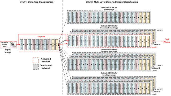
Aselective DCNNarchitecture, as shown in Fig.3, is pro-posed for low cost distorted image classification. The tiny CNN is used to classify the type and degree of image distor-tion. Then, based on the classification result, one dedicated DCNN is activated and used to classify the input image. The figure shows an example with three different types of distortions, each of which may distort a clean image by vary-ing degrees. Experiments with various large sets of distorted images and different types of possible tiny CNN architectures

FIGURE 2. MixQualNet architecture proposed in [12].

FIGURE 3. In the proposed selective DCNN architecture, onlyonededicated DCNN is active at any given time instant.

showed that a simple 4-layer CNN was sufficient to correctly classify, with close to 100% accuracy, all of the various distorted images in our test sets.

A. IMAGE DISTORTION

In this work, three types of distortions have been tested: Gaus-sian noise, GausGaus-sian blur, and low light. GausGaus-sian noise is

modeled assuming a low quality camera sensor, and an inter-face circuit affected by pool illumination and/or temperature variation is used [8], [9], [14]. For example, in a surveillance system that needs to operate 24 hours a day, low-quality camera sensors are often used because they require low power and limited storage space. Gaussian blur is modeled assum-ing that the camera is not focused properly on the object

FIGURE 4. Example SVHN image [16] after various levels of Gaussian noise, Gaussian blur, and low light.

[8], [9], [14]. Also, in the case of many low(or middle)-end type mobile phones, low quality cameras may be used, possibly resulting in an image that is blurred due to shaking or low resolution. Finally, low light is modeled assuming that the target image is not well illuminated. This is modeled by scaling the pixel values of the image to reduce the brightness of the image. A low light image could result when taking pictures at night or when using a camera in an autonomous vehicle that enters a tunnel.

In a realistic situation, it is reasonable to assume that the distortion degree as well as the distortion type of the image coming through the sensor are unknown. Therefore, in this work, three levels of distortion degree for each dis-tortion type are tested. Fig.4to6shows an example of how SVHN [16], CIFAR-100 [17], and Caltech-256 [18] images, respectively, would look like after these various distortion types and degrees are applied to Fig.5, and Fig.4, the stan-dard deviation of Gaussian noiseσnis chosen as 0.25, 0.5, and 0.75. The standard deviation of Gaussian blurσb is chosen as 1, 2, and 4. The scaling ratio of low lightsris chosen as 2, 3, and 4.

B. SELECTIVE DCNN

The operation of the selective DCNN consists of two steps. In the first step, a tiny CNN determines whether the input image is a clean or distorted image and the degree of dis-tortion. Then, in the second step, based on this decision, the dedicated DCNN for that specific distortion type and degree is activated and used to classify the input image. An example architecture of the proposed selective DCNN is shown in Fig.3. Unlike MixQualNet [12], shown in Fig.2, which requires all parts of the DCNN to be active, the active portions of a selective DCNN can be limited to one tiny CNN and one dedicated DCNN (shown using red dashed lines in Fig.3). Note also that a dedicated DCNN of this type can be

FIGURE 5. Example CIFAR-100 image [17] after various level of Gaussian noise, Gaussian blur, and low light.

thinner than the baseline DCNN for the same level of desired accuracy.

1) TINY CNN

The goals for the design of the tiny CNN are that (a) the size of the network should be small and (b) it should be able to correctly classify the types and degrees of distortions with extremely high accuracy. The tiny CNN in Fig.3categorizes clean and distorted images almost perfectly (for CIFAR-100 [17] and Caltech-256 [18], classification accuracies are 99.80% and 99.84%, respectively). The tiny CNN is obtained by repeatedly reducing a large network heuristically until the desired performance level is met. Fully connected layers are substituted with convolutional layers whenever possible.

The tiny CNN is a key part of the proposed selective DCNN architecture. Because the tiny CNN is trained to categorize the type and extent of distortion almost perfectly, it enables the selective DCNN to have high accuracy with low hardware cost. Different distortion types and degrees exhibit different features, which are recognized by the tiny CNN. For exam-ple, in the case of Gaussian noise and Gaussian blur, it is reported that there is a difference in the frequency domain analysis [14]. For low light images, the darker the modeling, the less the difference between the surrounding pixels. Other distortion types not considered here, but which may be added by the user later, could exhibit additional distinguishable features that would be captured by retraining the tiny CNN. 2) DEDICATED DCNN

The proposed selective DCNN, which uses separate dedicated networks for clean and distorted images, reduces the number of weight parameters without sacrificing classification accu-racy. As in [6], only 0.75, 0.5, and 0.25 times the number of input/output channels in the baseline DCNN are used. There-fore, the number of input/output channels of each dedicated

FIGURE 6. Example Caltech-256 image [18] after various level of Gaussian noise, Gaussian blur, and low light.

network is less than the baseline DCNN. The exact reduction rates achieved are described in SectionIII-C.

In Fig.3, there are a large number of weight parameters, but the number of parameters actually used for any single image is fewer than in the baseline network because only one dedicated DCNN is activated. Assuming a mobile embedded system with a typical DCNN accelerator and an image sensor, as shown in Fig. 7, all weight parameters are stored in an external DRAM and only one dedicated DCNN and tiny CNN are loaded into an on-chip buffer.

The proposed architecture can easily be extended to accommodate other types of distortions besides the ones tested in this work. To do so, one would need to use a dedicated DCNN for that specific distortion type. A network structure similar to the DCNNs used in this paper could be used, and the weights and other parameters for this new ded-icated DCNN could be trained with training images. The tiny CNN would also have to be retrained to be able to distinguish the new type of image distortion. From then on, the entire network would function in the same manner as before, and images with the new type of distortion would be classifiable with no significant increase in hardware cost or energy.

FIGURE 7. An example hardware design for a mobile embedded system.

C. HARDWARE COST MODEL

The cost of a DCNN can be evaluated in various ways. Hardware and energy usage costs are affected by the num-ber of weight parameters, the numnum-ber of MAC operations, the number of active processing elements (PEs), and the

data access energy required for the memories used per input image. By focusing on these factors, a new hardware cost metric is proposed in this section.

1) WEIGHT PARAMETERS AND MAC OPERATIONS

The number of weight parameters and MAC operations are the same as those proposed in [6]. The number of weight parameters and MAC operations can be computed as follows. WeightParams=DK×DK×kC×kM (1) NMAC =DK×DK×kC×kM×DF×DF (2) In (1) and (2),NMACrefers to the number of MAC accesses, DK is the height and width of a square shaped convolution kernel,Cis the number of input channels of the convolution filter, M is the number of output channels, and DF is the height and width of a square shaped feature map.k, which is the reduction ratio of channel depth to CNN, is set to 0.75, 0.5, and 0.25, as was also done in SectionIII-B.2. In the case of the first convolution layer of VGG16, for example, the input channel depth is 64 and the output channel depth is 64. Ifk is now set to 0.50, the input and output channel depths will change to 32. Accordingly, the weight parameters and number of MAC operations will be reduced by 0.25 times.

2) DATA ACCESS ENERGY

In the case of a mobile embedded system, which needs to be operated with limited power and memory capacity, a DCNN accelerator, instead of a general computing plat-form, is required for efficient DCNN processing. The energy required to access memory is a large portion of the total energy consumption of the DCNN accelerator [24]. Data access energy depends on the design characteristics of the DCNN accelerator. In this paper, data access energy is analyzed based on the Eyeriss architecture [24], which is described in Fig.7. Considering data reuse, the total energy of a DCNN accelerator can be computed as follows.

Etotal=eDRAM×NDRAM+ebuffer×Nbuffer

+_eRF×_NRF+_eMAC×_NMAC (3) In (3), e is the unit energy cost, which is summarized in Table1,Ncompis the count of memory accesses for memory components comp, and RFrefers to the register file. From the perspective of the DCNN accelerator implementation,N can vary greatly depending on how the data reuse pattern is determined. In this paper, it is assumed that a data reuse pattern with the least energy consumption is used in each layer among input reuse, output reuse, and weight reuse, as was also done in [25]. The values in Table 1 assume a 16-bit fixed point number system, which shows no accuracy degradation and is used in many architectures [24]–[26]. In Table1, the unit energy cost for DRAM access is obtained from [25], the unit energy cost for buffer access is extracted from CACTI 6.5 [27] with 65 nm CMOS technology, and the MAC operation unit energy cost is measured using Synopsys

TABLE 1.Energy cost for one 16-bit fixed point data item.

Design Compiler with a commercial 65 nm CMOS technol-ogy. RF unit access energy is assumed to be equal to a MAC as in [24].

When performing distorted image classification on mobile embedded systems, both classification accuracy and hard-ware costs need to be considered together. Wong [15] pro-posed such a metric, referred to as a NetScore. NetScore (denoted as) is computed as follows [15].

(N)=20log a(N)α p(N)βm(N)γ (4) In (4), N, a(N), p(N), and m(N) are the CNN architec-ture, CNN performance (image classification accuracy in this paper), the number of weight parameters, and the number of MAC operations, respectively.α,β, andγ are coefficients used to control the impact ofa(N),p(N), andm(N), respec-tively. As suggested in [15], the following coefficient values are used:α=2,β =0.5, andγ =0.5.

IV. EVALUATION

A. EXPERIMENTAL SETUP AND METHOD

In this paper, the SVHN [16], CIFAR-100 [17], and Caltech-256 [18] datasets are used for evaluation. Each type and level of distortion is applied to both training and test datasets. There are a total of 10 types of datasets, which consist of one clean dataset and 9 distorted datasets. The experiment is performed assuming the same number of instances of each type of dataset.

All three datasets listed above are commonly used for eval-uation of DCNN architectures [5], [12], [14]. In particular, SVHN [16] is a dataset of street view digits, which are impor-tant features that need to be recognized in future self-driving systems, collected from street view images. Clearly, distorted forms of these images will be common in real driving situ-ations. With almost 90% accuracy, distorted image classifi-cation of SVHN images are accurate enough to be used in practice. Used for general image classification, the CIFAR-100 [17] and Caltech-256 [18] datasets result in image classi-fication accuracy levels of 50–60% when distorted forms of images in those datasets are classified. Although this level of accuracy may be considered to be too low for general one-time classification, this type of distorted image classifi-cation could still be used for first-pass image classificlassifi-cation, used to mark images worthy of intensive scrutiny in noisy or adversarial situations.

As in [12], the baseline DCNN used is VGG16. The selec-tive DCNN architecture is created as a tiny CNN followed byndifferent VGG16 networks, wherenis the total number of dedicated DCNNs used, consisting of one DCNN for

TABLE 2. SVHN dataset [16] classification accuracies of dedicated DCNNs.

TABLE 3. CIFAR-100 dataset [17] classification accuracies of dedicated DCNNs.

clean images and one DCNN each for distorted images of each distortion type and degree considered. This proposed architecture is referred to as S-DCNN from now on.

The proposed method, S-DCNN, is compared to the fol-lowing three DCNNs: DCS-CNN [14], MixQualNet [12], and MobileNetV2 [13]. DCS-CNN [14] is a state-of-the-art DCNN for distorted image classification. DCS-CNN can only process Gaussian noise and Gaussian blur, so it will be com-pared separately with only those two noise types. MixQual-Net [12] is compared with three distortion types (Gaussian noise, Gaussian blur, and low light). MobileNetV2 [13], which was proposed for use in mobile or embedded devices (but not designed specifically for distorted image classifica-tion), is also compared for completeness as it is a recently published approach targeted for the same type of computing environment as S-DCNN.

S-DCNN and the comparison targets [12]–[14] are imple-mented using the PyTorch [28] Framework. The experiments are carried out using NVIDIA GTX1080 Ti GPUs. The experiments for CIFAR-100 datasets [17] are carried out with 8 GPUs and fine-tuned while varying the learning rate from 0.4 to 0.0004, which is decreased by 10×after 50 epochs, with a fixed batch size of 512. The experiments for Caltech-256 datasets [18] are carried out with 8 GPUs and fine-tuned while varying the learning rate from 0.01 to 0.0001, which is decreased by 10× after 50 epochs, with a fixed batch size of 128. The Caltech-256 dataset [18] is not divided into training and test datasets. Therefore, it is necessary to divide the training and test datasets. In this paper, these datasets are

divided using a ratio of four to one. Because the Caltech-256 dataset [18] contains different image sizes, image clas-sification is carried out after resizing each image to 256 by 256 pixels and then using a center crop at 224 by 224 pixels. All networks are trained with a stochastic gradient descent algorithm with momentum [29].

Implementation of multi-level distorted image classifica-tion for the distorted datasets is based on VGG16 [2]. Before checking the performance of the S-DCNN, it is necessary to check the top 1 percent accuracies of the dedicated DCNNs constituting the S-DCNN. Tables2to4summarize the classi-fication accuracies of the networks used with these dedicated DCNNs. In Tables2to4, the accuracy in the no distortion case is the classification accuracy of only clean images and the accuracies in the other cases are the classification accura-cies with only distorted images. The classification accuracy of the S-DCNN for each type of distortion is compared with the values shown in Tables 2 to 4. A description of the distortion degree is given in Section III-A. As shown in [6] and Tables2 to4, the classification accuracy is not drastically reduced even if the channel depth of DCNN is slightly reduced.

B. CASE STUDY 1: GAUSSIAN NOISE AND GAUSSIAN BLUR

The proposed S-DCNN is first compared with DCS-CNN [14], which is the most recent state-of-the-art DCNN architecture for classifying possibly distorted images. S-DCNN consists of the tiny CNN and the dedicated VGG16s

TABLE 4. Caltech-256 dataset [18] classification accuracies of dedicated DCNNs.

TABLE 5. Hardware costs and SVHN dataset [17] classification accuracies (DCS-CNN [14] vs. S-DCNNs).

FIGURE 8. NetScore [15] results of DCS-CNN [14] and S-DCNNs for distorted SVHN dataset [16] classification.

summarized in Tables 2 and3. Because DCS-CNN cannot classify low light images, only Gaussian noise and Gaussian blur distortions are considered.

For SVHN dataset [16] classification, the number of average activated weight parameters, the number of MAC operations, memory requirements, and top-1 accuracy of DCS-CNN [14] and the S-DCNN are summarized in Table5. As shown in Table 5, S-DCNNs always outperform DCS-CNN [14]. As shown in Fig.8, the S-DCNNs get up to 1.28× higher NetScores [15] than DCS-CNN [14].

For CIFAR-100 dataset [17] classification, the number of average activated weight parameters, the number of MAC operations, memory requirements, and top-1 accuracy of DCS-CNN [14] and the S-DCNN are summarized in Table6. As shown in6, all S-DCNNs have better performance than DCS-CNN in the number of weight parameter, the number of

TABLE 6.Hardware costs and CIFAR-100 dataset [17] classification accuracies (DCS-CNN [14] vs. S-DCNNs).

FIGURE 9. NetScore [15] results of DCS-CNN [14] and S-DCNNs for distorted CIFAR-100 dataset [17] classification.

MAC operations, required memory size, and top 1 classifi-cation accuracy. The results of the evaluation with NetScore appears in Fig.9. As shown in Fig.9, the S-DCNNs get up to 1.32×higher NetScores [15] than DCS-CNN [14]. This implies that S-DCNN is a better DCNN architecture when considering both the performance and hardware cost.

C. CASE STUDY 2: GAUSSIAN NOISE, GAUSSIAN BLUR, AND LOW LIGHT

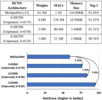
For SVHN dataset [16] classification, the S-DCNN is implemented based on the dedicated VGG16s summarized in Table2. Hardware costs and DCNN classification accu-racies of the S-DCNN and MixQualNet [12] are summa-rized in Table7. When comparing unpruned S-DCNN with k = 0.75 and MixQualNet [12], the number of weight parameters and MAC operations are reduced by 85.97% and

TABLE 7. Hardware costs and SVHN dataset [16] classification accuracies (MixQualNet [12] vs. S-DCNNs).

FIGURE 10. NetScore [15] results of MixQualNet [12] and S-DCNNs for distorted SVHN dataset [16] classification.

86.28%, respectively, while maintaining higher classification accuracy. Also, the NetScore [15] results, shown in Fig.10, demonstrate that the S-DCNNs have 1.29×to 1.60×higher scores than MixQualNet [8].

Based on the dedicated VGG16s summarized in Table3, the proposed S-DCNN is constructed and top 1 accuracies and hardware costs are obtained. For comparison, classifica-tion of distorted images for all cases with a single conven-tional VGG16 [2] and classification using MixQualNet [12] are also implemented. Details of the expert networks used with MixQualNet [12] are summarized in Table3. The num-ber of weight parameters and MAC operations, memory size, and top 1 classification accuracies are summarized in Table8. The S-DCNN, which includes both the tiny CNN and ded-icated VGG16, cases show higher classification accuracies than unpruned VGG16 and MixQualNet [12]. When com-paring unpruned S-DCNN withk = 0.50, which uses only half the channel depth of baseline VGG16 [2], and unpruned VGG16, the number of weight parameters and MAC oper-ations are reduced by 74.69% and 74.38%, respectively. When comparing unpruned S-DCNN with k = 0.50 and MixQualNet [12], the number of weight parameters and MAC operations are reduced by 93.68% and 93.61%, respectively. In addition, unpruned S-DCNN withk =0.50 requires only 7.4MiB of memory space. The NetScore [15] results, shown in Fig. 11, demonstrate that the S-DCNNs have 1.36×to 1.68×higher scores than MixQualNet [8].

Fig.12shows how much normalized data access energy per image is reduced using S-DCNN. The data access energy model is based on (3) and Table 1. As shown in Fig.12,

TABLE 8.Hardware costs and CIFAR-100 dataset [17] classification accuracies (MixQualNet [12] vs. S-DCNNs).

FIGURE 11. NetScore [15] results of MixQualNet [12] and S-DCNNs for distorted CIFAR-100 dataset [17] classification.

the energy consumption of the tiny CNN is negligible. Using unpruned S-DCNN with k = 0.50, which is more accu-rate than MixQualNet [12], data access energy is reduced by 91.92%.

Experiments are also performed on the Caltech-256 dataset [18] in the same way as in the previous exper-iments. Table 4 summarizes the classification accuracies of the networks used with these dedicated DCNNs for Caltech-256 dataset [18]. As in the CIFAR-100 experiments, the classification accuracy of the S-DCNN is based on the classification accuracies of the dedicated DCNNs in Table4. In Table4, it is shown that the size of the network is smaller and the classification accuracy is higher. In general, but not always [30], the larger the network size, the higher is the classification accuracy. Thus, a few exceptional cases, as can be seen in4, occur occasionally.

The top 1 classification accuracies with the Caltech-256 dataset [18] and hardware costs are summarized in Table9. Because the size of the Caltech-256 dataset [18] is much larger than the CIFAR-100 dataset [17], the fully-connected part for Caltech-256 dataset [17] classification is much larger. Therefore, there are differences in the number of weights and MAC operations for the Caltech-256 dataset [18]

FIGURE 12. Normalized data access energy of MixQualNet, baseline VGG16, and S-DCNNs for distorted CIFAR-100 dataset [17] classification.

TABLE 9. Hardware costs and caltech-256 dataset [18] classification accuracies (MixQualNet [12] vs. S-DCNNs).

FIGURE 13. NetScore [15] results of MixQualNet [12] and S-DCNNs for distorted Caltech-256 dataset [18] classification.

case and the CIFAR-100 dataset [17] case. In Table9, clas-sification accuracies of MixQualNet [12] are slightly higher than that of S-DCNN. However, the hardware costs of the proposed S-DCNNs are much lower than those of MixQual-Net [12]. The MixQual-NetScore [15] results are shown in Fig.13. All three S-DCNNs show 1.52×to 2.18×higher NetScores [15] than MixQualNet [12].

Fig.14shows how much normalized data access energy per image is reduced when using S-DCNN. Data access energy per image is reduced by up to 97.25% compared to

FIGURE 14. Normalized data access energy of MixQualNet, baseline VGG16, and S-DCNNs for distorted Caltech-256 dataset [18] classification.

MixQualNet [12]. Experimental results show that the S-DCNNs perform well on the Caltech-256 dataset [18].

There are several reasons why the S-DCNN can show a higher NetScore [15] than other comparison targets [12], [14]. First, because the tiny CNN can perfectly classify the type and degree of distortion, it can be used to activate the dedicated DCNN specific to each case. In a few cases, the accuracy may be lower than MixQualNet [12] because of its ensemble effect; however, MixQualNet requiresalldedicated DCNNs to be active whereas S-DCNN only requires one dedicated DCNN to be active. Second, the hardware cost is low because the size of the network activated in the actual on-chip hard-ware is smaller than that of the comparison targets [12], [14]. Thus, based on NetScores [15], which consider both accuracy and hardware cost, it can be seen that S-DCNN is signifi-cantly superior to the comparison targets [12], [14].

1) SELECTIVE DCNN WITH WEIGHT PRUNING

Magnitude-based weight pruning [19], which is commonly used for neural network size reduction, can be applied to the proposed S-DCNN to further reduce the network size. In this paper, it is assumed that 80% of the weights are pruned.

Hardware costs and CIFAR-100 dataset [17] classification accuracies of pruned cases are summarized in Table8 and Fig.12. If weight pruning is applied to the S-DCNN, the result is better with respect to all hardware costs. For the pruned S-DCNN withk = 0.50 case, the memory required is only 1.5MB, while the data access energy consumed is only 2.91% of the energy required for MixQualNet [12] despite main-taining higher classification accuracies than the comparison targets. In this paper, only weight pruning [19] is considered, but other network size reduction techniques, such as quanti-zation [31], will reduce hardware costs even further.

2) SELECTIVE DCNN WITH MIXEDK

In Table8 and9, in order to simplify the implementation, the sizes of the dedicated DCNNs are set to be the same. However, the dedicated DCNN can be varied in size to further lower the hardware costs. The dedicated DCNNs summarized in Table3are selected to have a higher classification accuracy

TABLE 10. Hardware costs and CIFAR-100 dataset [17] classification accuracies with MixQualNet, MobileNetV2, S-DCNN with Fixedk, and S-DCNN with mixedk.

than MixQualNet [12] with minimal hardware costs. The selected dedicated DCNNs are marked in bold.

As shown in Table3, it can be seen that 5 of the 10 ded-icated VGG16s are selected as VGG16 with k = 0.25. If all of the dedicated networks were of the same size, then networks scaled by 0.25 would not have been chosen. CIFAR-100 dataset [17] classification accuracies and average hard-ware costs of an S-DCNN architecture with mixedkvalues (corresponding to a mixture of different dedicated DCNN sizes, selected in order to minimize NetScore values) are summarized in Table10.

The hardware costs shown in this table include the costs for all activated weight parameters, MAC operations, and mem-ory requirements. As shown in Table10, unpruned S-DCNN with mixed k maintains higher accuracy than Net [12] with much lower hardware costs than MixQual-Net [12] and unpruned S-DCNN withk =0.50. The mixed k case results in higher NetScores [15] than the fixedk = 0.50 case because the reduction of the hardware cost is greater than the corresponding reduction in classification accuracy. In Table10, the decrease in the number of weight parameters is 35.90% compared to 4.11% for the accuracy reduction. Although the coefficients of the NetScores [15] used in this paper emphasize the accuracy (αis 2 and the others are 0.5), the decrease in hardware cost is still greater than the decrease in accuracy.

In order to compare S-DCNN with a DCNN designed to consider hardware costs only, the results of MobileNetV2 [13] are also summarized in Table10. MobileNetV2 [13] is a rela-tively small DCNN architecture compared to DCS-CNN [14] and MixQualNet [12], which are the other comparison targets used in this paper. Compared to MobileNetV2, it can be seen that the weight parameters are similar, the computation is less, and the classification accuracy is higher. A comparison of the NetScores [15] for the two types of methods are also shown in Fig.15. In Fig.15, unpruned S-DCNN with mixedkshows a higher NetScore [15] than MobileNetV2 [13].

3) SCALABILITY OF SELECTIVE DCNN

As mentioned in SectionIII-B.2, S-DCNN is highly scalable. The S-DCNN architecture can be easily extended by adding dedicated DCNNs and slightly modifying the tiny CNN. This scalability is an advantage when compared to other comparison target DCNNs [12]–[14], which are not as

scal-FIGURE 15. NetScore [15] results of MixQualNet, MobileNetV2 [13], and mixed S-DCNNs for distorted CIFAR-100 dataset [17] classification.

FIGURE 16. Example CIFAR-100 images [17] after new types of

distortions: (a) Gaussian blur with Gaussian noise, (b) Gaussian blur with standard deviation 3, and (c) salt and pepper noise.

able. In the case of DCS-DCNN [14], if the distortion degree is added, the number of average activated weight parameters increases. In the case of MixQualNet [12], an expert network needs to be added, which results in an increase in the number of activated weight parameters, or the existing expert network needs be retrained, which will result in longer training time than S-DCNN. In the case of MobileNetV2 [13], training will have to restarted from scratch to reflect the new distortion type.

To evaluate the scalability of S-DCNN, distortion cases are added and distorted image classification is conducted. The added distortion cases are Gaussian blur level 1 with Gaussian noise level 1, which represent a mixture of distortion types, Gaussian blur with standard deviation 3, which represents an unknown distortion level, and salt and pepper noise with probability of noisep=0.25, which represents an unknown distortion type. Fig. 16 shows examples of these types of distorted CIFAR-100 [17] images.

To extend the S-DCNN, the dedicated DCNNs within the S-DCNN can use the same hyperparameters as inIV-A. Since a dedicated DCNN has been added, the classifier part of the fully-connected layer of tiny CNN is modified to match the number of classes. In the case of the tiny CNN, the number of weight parameters and MAC operations increases by 1.12% and 0.03%, respectively, due to the increase in the number of classes to be classified, but this is negligible considering the size of the entire network.

Table11summarizes the distorted CIFAR-100 dataset [17] classification accuracies achieved with S-DCNN. As can be seen, reasonable accuracies are achieved with S-DCNN in all three cases.

TABLE 11. Other distorted CIFAR-100 dataset [17] classification accuracies.

V. CONCLUSION

For low hardware cost multi-level distorted image classi-fication in energy and memory constrained devices, this paper proposes a selective DCNN (S-DCNN) architecture composed of a tiny CNN, which classifies distortion types and degrees, and dedicated DCNNs, only one of which is activated and used to classify an input image. To evaluate the performance of the proposed S-DCNN, a comparison with previous state-of-the-art multi-level distorted image classifi-cation methods is conducted.

The experimental results using three popular image datasets show that S-DCNN has higher accuracy with up to 93.68%, 93.61%, and 91.92% lower memory requirements, MAC operations, and energy, respectively, than the previ-ous state-of-the-art DCNNs. In order to consider both CNN performance and hardware cost, a previously proposed com-prehensive metric, referred to as the NetScore, is also used. S-DCNN has up to 2.18×higher NetScores than the pre-vious state-of-the-art DCNNs. In addition, the performance of S-DCNN can be further improved by slight adjustments such as weight pruning. Finally, through our experiments, S-DCNN is shown to be highly scalable and adaptable to diverse image distortion types and degrees.

REFERENCES

[1] A. Krizhevsky, I. Sutskever, and G. E. Hinton, ‘‘ImageNet classification with deep convolutional neural networks,’’ inProc. Adv. Neural Inf. Pro-cess. Syst. (NIPS), 2012, pp. 1097–1105.

[2] K. Simonyan and A. Zisserman, ‘‘Very deep convolutional networks for large-scale image recognition,’’ 2014,arXiv:1409.1556. [Online]. Avail-able: https://arxiv.org/abs/1409.1556

[3] C. Szegedy, W. Liu, Y. Jia, P. Sermanet, S. Reed, D. Anguelov, D. Erhan, V. Vanhoucke, and A. Rabinovich, ‘‘Going deeper with convolutions,’’ in

Proc. IEEE/CVF Conf. Comput. Vis. Pattern Recognit. (CVPR), Jun. 2015, pp. 1–9.

[4] K. He, X. Zhang, S. Ren, and J. Sun, ‘‘Deep residual learning for image recognition,’’ in Proc. IEEE/CVF Conf. Comput. Vis. Pattern Recog-nit. (CVPR), Jun. 2016, pp. 770–778.

[5] G. Huang, Z. Liu, L. Van Der Maaten, and K. Q. Weinberger, ‘‘Densely connected convolutional networks,’’ inProc. IEEE/CVF Conf. Comput. Vis. Pattern Recognit. (CVPR), Jul. 2017, pp. 4700–4708.

[6] A. G. Howard, M. Zhu, B. Chen, D. Kalenichenko, W. Wang, T. Weyand, M. Andreetto, and H. Adam, ‘‘MobileNets: Efficient convolutional neu-ral networks for mobile vision applications,’’ 2017,arXiv:1704.04861. [Online]. Available: https://arxiv.org/abs/1704.04861?source=post_page [7] D. Velasco-Montero, J. Fernández-Berni, R. Carmona-Galán, and

Á. Rodríguez-Vázquez, ‘‘Optimum selection of DNN model and framework for edge inference,’’IEEE Access, vol. 6, pp. 51680–51692, 2018.

[8] S. Dodge and L. Karam, ‘‘Understanding how image quality affects deep neural networks,’’ in Proc. 8th Int. Conf. Qual. Multimedia Exper. (QoMEX), Jun. 2016, pp. 1–6.

[9] Y. Zhou, S. Song, and N.-M. Cheung, ‘‘On classification of distorted images with deep convolutional neural networks,’’ inProc. IEEE Int. Conf. Acoust. Speech Signal Process (ICASSP), Mar. 2017, pp. 1213–1217. [10] S. Diamond, V. Sitzmann, S. Boyd, G. Wetzstein, and F. Heide,

‘‘Dirty pixels: Optimizing image classification architectures for raw sensor data,’’ 2017, arXiv:1701.06487. [Online]. Available: https://arxiv.org/abs/1701.06487

[11] J. Kim, H. Zeng, D. Ghadiyaram, S. Lee, L. Zhang, and A. C. Bovik, ‘‘Deep convolutional neural models for picture-quality prediction: Challenges and solutions to data-driven image quality assessment,’’IEEE Signal Process. Mag., vol. 34, no. 6, pp. 130–141, Nov. 2017.

[12] S. F. Dodge and L. J. Karam, ‘‘Quality robust mixtures of deep neural networks,’’IEEE Trans. Image Process., vol. 27, no. 11, pp. 5553–5562, Nov. 2018.

[13] M. Sandler, A. Howard, M. Zhu, A. Zhmoginov, and L.-C. Chen, ‘‘MobileNetV2: Inverted residuals and linear bottlenecks,’’ in Proc. IEEE/CVF Conf. Comput. Vis. Pattern Recognit. (CVPR), Jun. 2018, pp. 4510–4520.

[14] Y. Byun, M. Ha, J. Kim, S. Lee, and Y. Lee, ‘‘Low-complexity dynamic channel scaling of noise-resilient CNN for intelligent edge devices,’’ in Proc. Design Autom. Test Eur. Conf. Exhib. (DATE), Mar. 2019, pp. 114–119.

[15] A. Wong, ‘‘Netscore: Towards universal metrics for large-scale performance analysis of deep neural networks for practical on-device edge usage,’’ 2018, arXiv:1806.05512. [Online]. Available: https://arxiv.org/abs/1806.05512

[16] Y. Netzer, T. Wang, A. Coates, A. Bissacco, B. Wu, and A. Y. Ng, ‘‘Reading digits in natural images with unsupervised feature learning,’’ inProc. NIPS Workshop Deep Learn. Unsupervised Feature Learn., 2011.

[17] A. Krizhevsky, ‘‘Learning multiple layers of features from tiny images,’’ M.S. thesis, Dept. Comput. Sci., Univ. Toronto, Toronto, Toronto, ON, Canada, 2009.

[18] G. Griffin, A. Holub, and P. Perona, ‘‘Caltech-256 object category dataset,’’ California Inst. Technol., Pasadena, CA, USA, Tech. Rep. 7694, 2007. [Online]. Available: http://authors.library.caltech.edu/7694

[19] S. Han, J. Pool, J. Tran, and W. Dally, ‘‘Learning both weights and con-nections for efficient neural network,’’ inProc. Adv. Neural Inf. Process. Syst. (NIPS), 2015, pp. 1135–1143.

[20] H. Li, A. Kadav, I. Durdanovic, H. Samet, and H. P. Graf, ‘‘Pruning filters for efficient convnets,’’ inProc. Int. Conf. Learn. Represent. (ICLR), 2017, pp. 1–13.

[21] S. Anwar, K. Hwang, and W. Sung, ‘‘Structured pruning of deep convolu-tional neural networks,’’ACM J. Emerg. Technol. Comput. Syst., vol. 13, no. 3, p. 32, 2017.

[22] Y. He, X. Zhang, and J. Sun, ‘‘Channel pruning for accelerating very deep neural networks,’’ inProc. Int. Conf. Comput. Vis. (ICCV), Oct. 2017, pp. 1389–1397.

[23] T.-J. Yang, Y.-H. Chen, and V. Sze, ‘‘Designing energy-efficient convolu-tional neural networks using energy-aware pruning,’’ inProc. IEEE/CVF Conf. Comput. Vis. Pattern Recognit. (CVPR), Jul. 2017, pp. 6071–6079. [24] Y.-H. Chen, J. Emer, and V. Sze, ‘‘Eyeriss: A spatial architecture for

energy-efficient dataflow for convolutional neural networks,’’ inProc. 43rd Int. Symp. Comput. Archit. (ISCA), Jun. 2016, pp. 367–379.

[25] F. Tu, S. Yin, P. Ouyang, S. Tang, L. Liu, and S. Wei, ‘‘Deep con-volutional neural network architecture with reconfigurable computation patterns,’’IEEE Trans. Very Large Scale Integr. (VLSI) Syst., vol. 25, no. 8, pp. 2220–2233, Aug. 2017.

[26] D. Kim, J. Ahn, and S. Yoo, ‘‘ZeNA: Zero-aware neural network acceler-ator,’’IEEE Design Test, vol. 35, no. 1, pp. 39–46, Feb. 2018.

[27] CACTI. Accessed: Sep. 17, 2019. [Online]. Available: http://www.hpl. hp.com/research/cacti/

[28] A. Paszke, S. Gross, S. Chintala, G. Chanan, E. Yang, Z. DeVito, Z. Lin, A. Desmaison, L. Antiga, and A. Lerer, ‘‘Automatic differentiation in pytorch,’’ inProc. NIPS Workshop Autodiff, 2017.

[29] I. Sutskever, J. Martens, G. Dahl, and G. Hinton, ‘‘On the importance of initialization and momentum in deep learning,’’ inProc. Int. Conf. Mach. Learn. (ICML), 2013, pp. 1139–1147.

[30] B. Zoph, V. Vasudevan, J. Shlens, and Q. V. Le, ‘‘Learning transferable architectures for scalable image recognition,’’ inProc. IEEE/CVF Conf. Comput. Vis. Pattern Recognit. (CVPR), Jun. 2018, pp. 8697–8710. [31] D. D. Lin, S. S. Talathi, and V. S. Annapureddy, ‘‘Fixed point quantization

of deep convolutional networks,’’ inProc. Int. Conf. Mach. Learn. (ICML), 2016, pp. 2849–2858.

MINHO HA (S’18) received the B.S. degree in electronic and electrical engineering from Sungkunkwan University, Suwon, South Korea, in 2015, and the M.S. degree in electrical engi-neering from the Pohang University of Science and Technology (POSTECH), Pohang, South Korea, in 2017, where he is currently pursuing the Ph.D. degree.

His current research interests include hardware efficient deep learning architecture, approximate computing, and embedded systems.

YOUNGHOON BYUN(S’18) received the B.S. degree in electronic and electrical engineering from the Pohang University of Science and Technology (POSTECH), Pohang, South Korea, in 2018, where he is currently pursuing the M.S. degree.

His current research interests include low power deep learning architecture, deep learning hardware accelerator, and embedded systems.

JEONGHUN KIM received the B.S. degree in electrical engineering from the Pohang University of Science and Technology (POSTECH), Pohang, South Korea, in 2018, where he is currently pursu-ing the Ph.D. degree.

His current research interests include embedded systems, network on chip, and hardware efficient deep learning architecture.

JAECHEOL LEE received the B.S. degree in electronic engineering from Kyungpook National University, Daegu, South Korea, in 2018. He is currently pursuing the M.S. degree in electrical engineering with the Pohang University of Sci-ence and Technology (POSTECH), Pohang, South Korea.

His current research interests include memory system, energy efficient hardware accelerator, and hardware efficient deep learning architecture.

YOUNGJOO LEE(M’14) received the B.S., M.S., and Ph.D. degrees in electrical engineering from the Korea Advanced Institute of Science and Tech-nology (KAIST), Daejeon, South Korea, in 2008, 2010, and 2014, respectively.

He was with Interuniversity Microelectronics Center (IMEC), Leuven, Belgium, from 2014 to 2015, where he researched reconfigurable SoC platforms for software-defined radio systems. From 2015 to 2017, he was with the Faculty of the Department of Electronic Engineering, Kwangwoon University, Seoul, South Korea. Since 2017, he has been an Assistant Professor with the Department of Electrical Engineering, POSTECH, Pohang, South Korea. His current research interests include the algorithms and architectures for embedded processors, intelligent mobile systems, advanced error correction codes, and next-generation communication systems.

SUNGGU LEE (M’88) received the B.S.E.E. degree (Hons.) from the University of Kansas, Lawrence, KS, USA, in 1985, and the M.S.E. and Ph.D. degrees from the University of Michi-gan, Ann Arbor, MI, USA, in 1987 and 1990, respectively.

He was an Assistant Professor with the Depart-ment of Electrical Engineering, University of Delaware, Newark, DE, USA. From 1997 to 1998, he was a Visiting Scientist with the IBM T. J. Watson Research Center, Yorktown Heights, NY, USA. From 2005 to 2006, he was a Visiting Researcher with the DREAM Laboratory, University of California at Irvine, Irvine, CA, USA. From 2012 to 2013, he was a Visiting Researcher with Samsung Electronics, Suwon, South Korea. Since 1991, he has been a full-time Professor with the Department of Electrical Engineer-ing, Pohang University of Science and Technology (POSTECH), Pohang, South Korea. His current research interests include deep neural networks, approximate computing, parallel processing, and fault-tolerant design.