Transformation and Ensembles
Jason Andrew Lines
A Thesis Submitted for the Degree of Doctor of Philosophy
University of East Anglia School of Computing Sciences
February 2015
c
This copy of the thesis has been supplied on condition that anyone who consults it is understood to recognise that its copyright rests with the author and that use of any information derived there from must be in accordance with current UK Copyright Law. In addition, any quotation or extract must include full attribution.
The problem of time series classification (TSC), where we consider any real-valued or-dered data a time series, offers a specific challenge. Unlike traditional classification problems, the ordering of attributes is often crucial for identifying discriminatory fea-tures between classes. TSC problems arise across a diverse range of domains, and this variety has meant that no single approach outperforms all others.
The general consensus is that the benchmark for TSC is nearest neighbour (NN) classifiers using Euclidean distance or Dynamic Time Warping (DTW). Though concep-tually simple, many have reported that NN classifiers are very difficult to beat and new work is often compared to NN classifiers. The majority of approaches have focused on classification in the time domain, typically proposing alternative elastic similarity mea-sures for NN classification. Other work has investigated more specialised approaches, such as building support vector machines on variable intervals and creating tree-based ensembles with summary measures.
We wish to answer a specific research question: given a new TSC problem without any prior, specialised knowledge, what is the best way to approach the problem? Our thesis is that the best methodology is to first transform data into alternative represen-tations where discriminatory features are more easily detected, and then build ensemble classifiers on each representation. In support of our thesis, we propose an elastic ensemble classifier that we believe is the first ever to significantly outperform DTW on the widely-used UCR datasets. Next, we propose the shapelet-transform, a new data transformation that allows complex classifiers to be coupled with shapelets, which outperforms the orig-inal algorithm and is competitive with DTW. Forig-inally, we combine these two works with with heterogeneous ensembles built on autocorrelation and spectral-transformed data to propose a collective of transformation-based ensembles (COTE). The results of COTE are, we believe, the best ever published on the UCR datasets.
First and foremost I would like to thank my supervisor, Dr. Anthony Bagnall, and my family. Without Tony’s invaluable advice and guidance, and the continued support and encouragement from my parents and close family, the work in this thesis would not have been possible.
I would like to thank my examiners, Prof. Niall Adams and Dr. Beatriz de la Iglesia, for their patience and insight while examining this thesis. I would also like to thank Tony’s other PhD students during my study, Jon and Luke, and my second supervisor, Dr. Richard Harvey. Additional thanks go to my peers at UEA, particularly those who I shared a lab with for four years (and everyone in the graphics lab since I spent as much time in there too!). I’d also like to thank all of the staff and students in the School of Computing Sciences at UEA who have supported me throughout my studies. Special mentions go to Felix and Dom for being a constant source of entertainment and distraction, Ollie for providing the cake and enough surreal moments to last a lifetime, Luke for his 80’s pop-rock outbursts, and everyone from CMP and ITCS that played football on Thursdays.
Finally, I’d like to thank some important people outside of university. Thank you to Shane Migliore and everyone at Apple for helping make Austin my home for four months at the end of my PhD. As well as new friends, I’d like to thank those who have always been there for me. In particular, thank you to Bedford, Beth, Danny, David, Emma, Faires, James, Jim, and Sarah. Without you, I would have gone crazy a long time ago. Also, thank you to Freddie and Ollie (my dogs) for not eating my thesis, and a special thank you to my mother for painstakingly helping me with the final round of proofreading!
In loving memory of Kenneth Thomas Deare.
Acknowledgements ii List of Publications v 1 Introduction 1 1.1 Motivation . . . 2 1.2 Contributions . . . 3 1.3 Thesis Organisation . . . 6
2 Technical Background and Related Work 7 2.1 Time Series Classification . . . 7
2.2 Comparing Classifiers . . . 9
2.3 Nearest Neighbour Classification in the Time Domain . . . 11
2.3.1 k-Nearest Neighbour (k-NN) Classifiers . . . 12
2.3.2 Euclidean Distance . . . 12
2.3.3 Dynamic Time Warping . . . 13
2.3.4 Derivative Dynamic Time Warping . . . 16
2.3.5 Weighted Dynamic Time Warping . . . 17
2.3.6 Longest Common Subsequence Distance . . . 17
2.3.7 Edit Distance with Real Penalty . . . 19
2.3.8 Time-Warp Edit Distance . . . 20
2.3.9 Move-Split-Merge . . . 20
2.4 Standard Classification Algorithms . . . 22
2.4.1 Na¨ıve Bayes . . . 23
2.4.2 C4.5 Decision Tree . . . 23
2.4.3 Support Vector Machine . . . 24
2.4.4 Random Forest . . . 25
2.4.5 Rotation Forest . . . 26
2.5 Ensemble Classifiers . . . 26
2.5.1 Bagging . . . 27
2.5.2 Boosting . . . 27
2.5.3 Other Ensembles in the TSC Literature . . . 28
2.5.4 A Simple Heterogeneous Ensemble . . . 28
2.6.1 Summary Statistics and Feature Extraction . . . 31
2.6.2 Compression/Approximation-based Transforms . . . 33
2.6.3 Transformation into Alternative Data Spaces . . . 35
3 Data 37 3.1 UCR Time Series Data Repository . . . 37
3.2 Electricity Consumption Problems . . . 38
3.2.1 Visual Energy Trail (VET) Data . . . 39
3.2.2 Household Energy Study (HES) Data . . . 41
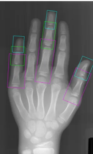
3.3 Hand Outline Datasets . . . 42
3.3.1 Data Preparation . . . 42
3.4 MPEG-7 Problems . . . 45
3.5 Caenorhabditis elegans . . . 46
4 Time Series Similarity with Alternative Representations 49 4.1 Global Similarity in Shape: Power Spectrum . . . 50
4.1.1 Motivational Example: Electrical Devices . . . 51
4.2 Local Similarity in Shape: Shapelets . . . 51
4.2.1 Shapelet Extraction . . . 53
4.2.2 Assessing Shapelet Candidates . . . 54
4.2.3 Shapelet Similarity . . . 54
4.2.4 Shapelet Quality Measures . . . 54
4.2.5 Example: MPEG7 Data . . . 57
4.3 Similarity in Change: Autocorrelation Transform . . . 57
5 Time Domain Classification: Current Benchmarks and a New State-of-the-art 62 5.1 Datasets . . . 64
5.2 Nearest Neighbour Classification: Hard to beat, or a misconception? . . . 64
5.2.1 Experimental Procedure . . . 65
5.2.2 Results . . . 66
5.3 Configuring Distance Measures with Nearest Neighbour Classifiers . . . . 67
5.3.1 Setting the Number of Neighbours . . . 68
5.3.2 Parameterising Distance Measures . . . 70
5.3.3 Concluding Remarks . . . 71
5.4 Comparison of Elastic Distance Measures . . . 72
5.4.1 Elastic Measure Experimental Design . . . 72
5.4.2 Classification Results . . . 73
5.4.3 A Priori Detection of the Best Measure . . . 75
5.4.4 Timing Comparison . . . 78
5.5 Combining Elastic Measures: The Elastic Ensemble . . . 78
5.5.1 Measure Divergence . . . 80
5.5.4 Elastic Ensemble vs. Other Approaches . . . 84
5.6 Conclusions . . . 87
6 Shapelet Domain Classification: The Shapelet Transform 89 6.1 Introduction . . . 89
6.2 Datasets . . . 91
6.3 The Shapelet Transform . . . 92
6.3.1 Extracting thek Best Shapelets . . . 92
6.3.2 Data Transformation . . . 94
6.3.3 Settingk in the Shapelet Transform . . . 95
6.3.4 Setting Shapelet Length Parameters . . . 96
6.4 Alternative Shapelet Quality Measures . . . 97
6.5 Experimental Design . . . 101
6.6 Results . . . 101
6.6.1 Embedded Shapelets vs. Transformed Shapelets . . . 101
6.6.2 Using F-stat with the Shapelet Transform . . . 103
6.6.3 Alternative Classifiers with Shapelet-transformed Data . . . 105
6.6.4 Shapelet Selection . . . 107
6.6.5 Exploratory Data Analysis . . . 107
6.6.6 Comparison to Alternative Approaches . . . 110
6.7 Conclusions . . . 112
7 The Collective of Transformation-based Ensembles 114 7.1 Datasets . . . 115
7.2 Transformation-based Ensembles . . . 116
7.2.1 Heterogeneous Ensemble . . . 116
7.2.2 Time Domain Classification with the Elastic Ensemble . . . 118
7.3 Results Using a Single Ensemble: Flat-COTE . . . 118
7.4 Case Study: Classifying Caenorhabditis elegans . . . 121
7.5 Comparison to Other Approaches . . . 122
7.6 Alternative Ensemble Designs . . . 127
7.6.1 Best Internal Ensemble . . . 127
7.6.2 Weighted Internal Ensembles . . . 129
7.6.3 Subset of Internal Ensembles . . . 131
7.7 Conclusion . . . 132
8 Conclusions and Future Work 134 8.1 Discussion of Contributions . . . 135
8.2 Future Work and Extensions . . . 136
Bibliography 138
As First Author
• Jason Lines, Anthony Bagnall, Patrick Caiger-Smith, and Simon Anderson. Classification of household devices by electricity usage profiles. InIntelligent Data Engineering and Automated Learning-IDEAL 2011, pages 403–412. Springer Berlin Heidelberg, 2011.
• Jason Lines, Luke M Davis, Jon Hills, and Anthony Bagnall. A shapelet transform for time series classification. In Proceedings of the 18th ACM SIGKDD Inter-national Conference on Knowledge Discovery and Data Mining, pages 289–297. ACM, 2012.
• Jason Lines and Anthony Bagnall. Alternative quality measures for time series shapelets. InIntelligent Data Engineering and Automated Learning-IDEAL 2012, pages 475–483. Springer Berlin Heidelberg, 2012.
• Jason Lines and Anthony Bagnall. Ensembles of elastic distance measures for time series classification. In Proceedings of the 14th SIAM International Conference on Data Mining (SDM), pages 524–532. 2014.
• Jason Lines and Anthony Bagnall. Time series classification with ensembles of elastic distance measures. Data Mining and Knowledge Discovery, pages 1–28, 2014.
As Co-author
• Anthony Bagnall, Luke M Davis, Jon Hills, and Jason Lines. Transformation based ensembles for time series classification. In Proceedings of the 12th SIAM International Conference on Data Mining (SDM), pages 307–318. SIAM, 2012.
• Luke M Davis, Barry-John Theobald, Jason Lines, Andoni Toms, and Anthony Bagnall. On the segmentation and classification of hand radiographs. International Journal of Neural Systems, 22(05), 2012.
• Jon Hills, Jason Lines, Edgaras Baranauskas, James Mapp, and Anthony Bag-nall. Classification of time series by shapelet transformation. Data Mining and Knowledge Discovery, 28(4):851–881, 2014.
Introduction
Time series data, which we consider as any real-valued ordered data, arise across many domains. These include, but are not limited to: econometrics, medicine, weather, motion capture, image processing, computational biology, signal processing, and pattern recog-nition. The problem of time series classification (TSC) is a specialisation of the more general classification problem; the objective of classification is, given a new test instance of data, can the category, orclass, of this observation be determined from characteristics that have been extracted from a set of previously observed training data with known class labels?
To an extent, all classification problems rely on identifying explanatory features within the data, then using a measure of similarity to quantify the relationships between them to inform the decision process. TSC offers a specific challenge, as the ordering of the data may be crucial in discriminating between class values. For example, the data may have an embedded structure, such as autocorrelation, or trends. To this end, traditional classification approaches may not be best suited to TSC problems. This has prompted many different approaches for solving TSC problems to be proposed in the literature [9, 58, 20, 49, 107, 80, 106, 50, 55]. These range from the most generic end of the spectrum (using standard classification algorithms on time series data and ignoring the dependency between attributes), to the most specialised (creating bespoke problem-specific solutions). There are also many other solutions in between, such as using support vector machines built on variable intervals [93], or tree-based ensembles built on summary measures [34].
However, it has been observed many times in the literature that, in general, a nearest neighbour classifier using a measure of time series similarity is very difficult to beat. This is noted succinctly by Batistaet al.[10], who state that ‘there is a plethora of
tion algorithms that can be applied to time series; however, all of the current empirical evidence suggests that simple nearest neighbour classification is very difficult to beat’. One of the simplest approaches for solving TSC problems is to to use a one-nearest neighbour (1-NN) classifier with Euclidean distance. However, the widely-accepted benchmark in TSC currently is to use a 1-NN classifier coupled with Dynamic Time Warping (DTW) with a warping window set through cross-validation (CV) [21,47,34].
1.1
Motivation
Given a new TSC problem to solve, the optimal solution will most likely be achieved by creating a custom, bespoke solution that is tailor-made to the problem at hand. However, this approach is typically very time and resource consuming, and will likely result in a solution that is very difficult (or impossible) to generalise to other problems. Theno free lunch theorem [105] applies to many fields, and TSC is not immune; there is no single solution that is optimal for all problems. As already discussed, the literature argues that, in general, nearest neighbour classification isvery difficult to beat, and DTW with a 1-NN classifier is considered the current gold-standard for TSC. With this in mind, when presented with a new TSC problem the sensible approach would be to build a NN classifier with DTW. However, we believe this approach is na¨ıve.
Firstly, there are many different types of similarity that can be observed between time series data. For example, series could change at similar points in time (time-based similarity), or they could have similar underlying curves or trends (global shape-based similarity). Also, the series could be similar in the ways that they change due to their internal structures, such as the autocorrelation of the series and how the values of subsequent readings are influenced by previous readings (change-based similarity). Additionally, the presence of localised common subsequences could be indicative of class membership. An approach using 1-NN and DTW would be well suited to measuring time-based similarity, but may struggle to identify the best discriminatory features in the other three cases. It would therefore be desirable if we could determine a priori which type of similarity should be used for a new problem.
Secondly, even if using a simple 1-NN approach, there are many alternative similarity measures that have been proposed in the literature that could be used in place of DTW. Many are claimed to be at least as effective as DTW, and in some cases it is stated that the alternatives are more effective. However, evaluation methods are inconsistent and are sometimes based on simple head-to-head results and anecdotal evidence. It is currently unclear whether any alternatives are truly more effective than DTW, but it is clear that
various alternatives capture similarity differently to DTW (for example, edit distance-based approaches [25,26,79]). It would be desirable to know in advance whether DTW is the most appropriate measure to use with a 1-NN classifier for a given problem, or even if it is possible to combine the output of multiple measures to make a more diverse and informed decision. This leads to the research question that has influenced the work throughout this thesis: given a new TSC problem with no prior, specialised knowledge, what is the best way to approach classification?
In [3], it was shown that a simple way to gain improvement in TSC problems is to transform data into alternative domains where where discriminatory features are more easily detected. We use this as a starting point; our thesis is that the best way to ap-proach a TSC problem without any prior specialised knowledge is to first transform data into alternative representations where discriminatory features are more easily detected. This would potentially allow algorithms to not only measure similarity between series in the time domain, but also consider similarity in change, global-shape, and local-shape. Then, we believe that through using transparent ensemble schemes, we can build en-semble classifiers in each of these domains to form constituent enen-sembles in a diverse collective of transformation-based ensembles. Many algorithms embed data transforma-tion within classificatransforma-tion algorithms. We believe that by transforming data independently of classifiers, and by utilising simple ensemble voting schemes, we can produce a very ac-curate and transparent classifier that can outperform the benchmark set by DTW 1-NN, and provide a framework that can easily be extended in future work to add additional classification algorithms and data representations.
1.2
Contributions
In pursuit of providing support for our thesis, numerous experiments were carried out and novel algorithms were proposed. The main contributions of this thesis are as follows:
• Time series classification in the time domain. An extensive study was carried out using 75 datasets to evaluate whether DTW with warping set through cross-validation (DTWCV) is still the benchmark for TSC. Initially this investigation focused on whether DTW was hard to beat through a comparative study between various standard classification algorithms and 1-NN classifiers implemented using Euclidean distance and DTW with a full window. After establishing that none of these classifiers significantly outperformed DTW, an investigation was carried out to determine the best configuration for DTW with NN classifiers, including whether
the neighbourhood size of the NN classifier or window width of the DTW measure should be set through cross-validation. After answering these questions and rec-ommending that DTW be implemented with a warping window set through cross-validation and one nearest neighbour, we carried out a comparison of DTWCV to alternative elastic similarity measures that have been proposed in the literature, including approaches such as Weighted DTW [58], Move-Split-Merge [101], and Time Warp Edit Distance [79]. Over the 75 datasets tested, we found that no alternative significantly outperformed DTWCV, concluding that DTWCV with 1-NN was still the benchmark in TSC. However, through investigating the alternative elastic measures, we demonstrated that while the measures did not produce sig-nificantly different accuracies, they did produce sigsig-nificantly different predictions. This motivated an investigation into using simple ensemble schemes to build an ensemble classifier with each of the elastic measures. The resulting classifier, the elastic ensemble (EE), is significantly more accurate than DTWCV over the 75 datasets. Additionally, the EE is significantly more accurate than DTW on the 46 UCR datasets that are widely throughout the TSC literature for evaluating new algorithms. This result is noteworthy, as we believe this is the first time a classifier has ever outperformed DTWCV on the UCR TSC problems. This work is reported in Chapter 5and was published in [75,76].
• A novel shapelet transform. As outlined in our thesis, we believe that the best approach for TSC is to evaluate similarity in additional domains to the time do-main. One area of time series similarity that is currently under represented in the literature is similarity in local-shape. A recent approach, time series shapelets [107], was proposed to match series according to common local patterns through extract-ing discriminatory subsequences to build a decision tree classifier. This approach was designed to produce intuitive results, but restricts shapelets by embedding them within a classifier. We use this as a starting point to create a new time series transformation that mitigates the limitations of a shapelet decision tree ap-proach by extracting the top k shapelets from a dataset in a single pass through using a novel caching algorithm. The extracted shapelets are used to transform series into a new k-dimensional representation, where each feature is the distance between a shapelet and the input series. The result of this transform is that the new representation can be applied to any standard classification algorithm, facil-itating classification based on local shape-based similarity. We demonstrate that using the shapelet transform with popular classification algorithms such as support
vector machines and random forest significantly outperforms the original shapelet tree-based approach, and we also provide information to show that classification accuracy can be greatly improved for problems that are not well-suited to the time domain when compared against DTWCV. We also extend our work to consider alternative measures of shapelet quality that are more suited to the transformation approach, and demonstrate that they are significantly faster for shapelet extraction than the information gain measure used in the original approach. Finally, we pro-duce a case study using a popular UCR dataset to mirror the case study provided in the original shapelet work to demonstrate that our shapelet transform retains the intuition provided by the original approach, and may also allow for greater insight to be gained. This work is described in Chapter6and was published in [78,74,52].
• COTE: The collective of transformation-based ensembles for time series classification. This work builds upon the conclusion in [3] that the simplest way to improve accuracy for TSC problems is to transform data into alternative do-mains where discriminatory features are more easily detected. This is extended by creating a collective of ensemble classifiers built in four domains: time, local shape, global shape, and change. We use the elastic ensemble proposed in Chapter 5 for time domain classification, and we create a simple heterogeneous ensemble to ap-ply to transformed data in the remaining three domains. For representing local shape-based similarity, we transform series using the shapelet transform that we propose in Chapter 6. For global shape-based similarity we transform data us-ing the power spectrum, and for change, we use autocorrelation-based transforms. Through extensive experimentation on 72 datasets, including all of the 46 UCR datasets, we demonstrate that the simple collective formed by including all clas-sifiers in one ensemble is significantly more accurate than any other previously published TSC algorithm, including the EE. We call this classifier the collective of transformation-based ensembles (COTE), and the results provided by COTE provide strong support for our thesis. Finally, after proposing and testing the ini-tial configuration for COTE, we propose alternative versions using weighting and selection schemes in pursuit of adding extra insight to results without reducing accuracy. This work is described in Chapter 7, and the results of the COTE are, we believe, the best ever published on the UCR datasets.
1.3
Thesis Organisation
The remainder of this thesis is organised as follows. In Chapter 2, a thorough review of the TSC literature is carried out, including specific emphasis on nearest neighbour clas-sification in the time domain with DTW and other alternative elastic distance measures. In Chapter 3 we introduce the datasets that are used throughout this thesis, including new problems that we have provided and shared with the TSC community for the first time. Chapter 4 discusses transformation approaches for time series to allow for simi-larity to be assessed in alternative domains, while Chapter5 focuses specifically on the time domain and culminates in the proposal of the EE. Chapter6moves away from time domain similarity to propose a novel transform to capture similarity in local-shape: the shapelet transform. The findings in Chapter 5 and 6 are then combined in Chapter 7 where the COTE is proposed and tested, demonstrating that forming a collective of ensemble classifiers built on different time series representations can significantly outper-form DTWCV, and any other classifier that we know of, across our test set of 72 datasets and the UCR data. Finally, in Chapter 8, we conclude this thesis by summarising the contributions of this work and discussing possible future direction.
Technical Background and
Related Work
This chapter introduces the relevant background materials for this thesis. We motivate and introduce the problem of time series classification (TSC), and present a review of the leading solutions that have been proposed in the literature. Specifically, we focus on the common benchmark technique of using simple nearest neighbour (NN) classifiers with Euclidean distance Dynamic Time Warping (DTW) to solve the problem in the time domain, and explore potential alternative elastic measures that can be combined with NN classifiers. Following this, we investigate more complex solutions that have been introduced in the literature, including approaches built on transforming data into other domains and combining decisions of multiple classifiers.
2.1
Time Series Classification
Many problems exist in the time series data mining literature, including classification, clustering, indexing, and querying. In this thesis, we focus solely on the problem of time series classification (TSC). We define a time series as a sequence of data that is typically recorded in temporal order at fixed time intervals. For the problem of TSC, we use a set of ntime series
T ={T1, T2, ..., Tn} (2.1)
where each series consists of m real-valued ordered observations
Ti=< ti,1, ti,2, ..., ti,m > (2.2)
and a class valueci. GivenT, the TSC problem is to find a function that maps from the
space of possible time series to the space of possible class values. For simplicity, in our definition we assume that all series ofT are the same length.
A key feature that distinguishes TSC problems from general classification problems is that the features within the data that discriminate between class values are often embedded within the inter-relationship structure of the data. In generic classification problems, attributes of the data are often independent; in TSC problems, the ordering and structure of the data often play a crucial role in uncovering features that define class relationships.
The nature of TSC problems means that the representation of the data is a crucial part of any TSC algorithm, and all TSC approaches rely to an extent on measures of similarity between data. There are three broad categories of TSC similarity that appear in the literature:
• Similarity in time can be observed when series from a class are observations of an underlying common curve in the time dimension. When there is no noise in the observation, correlation-based measures or the Euclidean distance can be used to effectively measure similarity between series. When there is noise in the time dimension or slight phase-shift, elastic distance measures can be used. Dy-namic time warping (DTW) is by far the most popular of such measures in the literature [62,91,35,61,64,90,49].
• Similarity in shapeis when class membership is characterised by a common shape in the data that is phase-independent. This can cover two such scenarios: firstly, if the common shape involves the whole series, but the shape is shifted between instances of the same class, transforming the data into the frequency domain can uncover discriminating features [22, 57]. Secondly, if the common shape is local and embedded within instances of the same class, subsequence techniques such as shapelets [107,108,80,89] can measure shape-based similarity accurately without being affected by noise throughout the rest of the series.
• Similarity in change is where the discriminatory features of a dataset are em-bedded within the autocorrelation structure of the data. This type of similarity is the least covered in the literature, but can be employed for TSC by transforming series into the change domain through the use of autocorrelation-based transforms, or by applying autoregressive moving average models (ARMA) to the data and judging similarity on model parameters [27,4,5].
In this chapter we survey and review the TSC literature across each of these types of similarity. Similarity in time is by far the most represented of the three in the TSC liter-ature, and this is reflected by the extensive discussion of nearest neighbour classification with alternative elastic similarity measures in Section2.3. A discussion of popular TSC algorithms follows in Section 2.4, including approaches that involve transforming data into other domains to uncover similarity. In Section2.5, the process of combining multi-ple algorithms to form ensemble classifiers is discussed and motivated with an exammulti-ple of a heterogeneous ensemble in the time domain. Before exploring specific TSC algorithms however, we must introduce a methodology for consistently comparing classifiers across many datasets.
2.2
Comparing Classifiers
In order to test the thesis outlined in Chapter 1, it is necessary to objectively compare classification algorithms over many datasets. In the literature it is common to base support for new algorithms on anecdotal evidence or simple win/loss statistics. We wish to be more thorough in our analysis during this thesis, and adopt the procedure outlined in [33] to test for statistical significance between classifiers. The approach is based on a two-stage rank-sum test using the non-parametric equivalent to analysis of variance (ANOVA).
The first stage of the approach tests the null hypothesis that there is no significant difference between the average ranks ofkclassifiers onndatasets, against the alternative hypothesis that at least one classifier’s mean rank is different. Given M, the k by n
matrix of classification accuracies where mi,j is the accuracy of the ith classifier on the
jth dataset, M = m1,1 m1,2 · · · m1,n m2,1 m2,2 · · · m2,n .. . ... . .. ... mk,1 mk,2 · · · mk,n (2.3)
the first step is to calculate the corresponding n by k matrix R, where ri,j is the rank
averaged: R= r1,1 r1,2 · · · r1,n r2,1 r2,2 · · · r2,n .. . ... . .. ... rk,1 rk,2 · · · rk,n (2.4)
From R the average rank of classifier j is calculated as ¯rj =
Pn i=1ri,j
n . To test the
hypothesis, the Friedman statisticQ,
Q= 12n k(k+ 1) · k X j=1 ¯ rj2− k(k+ 1)2 4 (2.5)
can be approximated using a Chi-squared distribution with (k−1) degrees of freedom to test the null hypothesis that there is no difference between the mean ranks of the classifiers. However in [33], Demˇsar notes that this calculation is often conservative, and proposes using the following statistic:
F = (n−1)Q
n(k−1)−Q, (2.6)
that, under the null hypothesis, follows an F distribution with (k−1) and (k−1)(n−
1) degrees of freedom. If the result of this calculation is that we can reject the null hypothesis, resulting in at least one classifier having a significantly different average rank, the second stage of the approach proposed by Demˇsar involves performingpost-hoc pair-wise Nemenyi tests to observe where differences occur. The test states that the average ranks of two classifiers are significantly different if they differ by at least the critical difference, calculated as:
CD =qa
r
k(k+ 1)
6n , (2.7)
whereqa is based on the studentised range, where the difference between the largest and
smallest values in the sample is measured in units of standard deviation. By comparing all classifiers in this way, Demˇsar proposes that a critical difference diagram can be cre-ated to effectively summarise the results. This is formed by creating a diagram where the average ranks for each classifier are labelled on a numerical range, and classifiers that are not significantly different from one another are organised intocliques. A clique is represented by a solid black line, and allows for simple interpretation of results by
observing whether classifiers are within a common clique. If two classifiers do not belong to at least one common clique, the average ranks of the classifiers are significantly differ-ent. A motivational example of a critical difference diagram is presented in Figure 2.1. We use critical difference diagrams throughout this thesis to compare results of multiple classifiers over multiple datasets.
CD 5 4 3 2 1 1.7083 Classifier A 2.3125 Classifier B 2.9583 Classifier C 3.3958 Classifier D 4.625 Classifier E
Figure 2.1: An example of a critical difference diagram with five fictional classifiers. The critical difference in this diagram is 1.1228; The average ranks of Classifier A and Classifier B do not differ by more than the critical difference, so the ranks are not significantly different. However, Classifier A and Classifier C are not within the same clique, so it is demonstrated that they are significantly different.
2.3
Nearest Neighbour Classification in the Time Domain
Numerous algorithms and approaches have been proposed in the literature for solving TSC problems. However, as eluded to in Chapter 1, currently there has been no conclu-sive evidence reported to suggest that any technique is significantly more accurate than using a simple nearest neighbour (NN) classifier for TSC. This is reinforced by Batista et al. in [9], who state that ‘there is a plethora of classification algorithms that can be applied to time series; however, all of the current empirical evidence suggests that simple nearest neighbor classification is very difficult to beat’. The sentiment of this statement is echoed in various other work throughout the literature, with the general consensus that NN classifiers combined with either Euclidean distance or Dynamic Time Warping are the current benchmark for TSC [21,47,34].
2.3.1 k-Nearest Neighbour (k-NN) Classifiers
Thek-NN classifier is one of the oldest, simplest, and most commonly used classification algorithms that is fundamental to many TSC approaches, particularly approaches in the time domain (for example, [60,92,106,79,9, 21,47,101]). The classifier was first documented in [39] and is intuitively very simple to implement for TSC problems. Given a set of labelled training time seriesT and a query seriesq with an unknown class value, the objective is to find the k most similar series to q in T, where 1 ≤ k ≤ n. The predicted class valuec∗ forq is selected as the modal value of thek nearest neighbours. The value fork is often set as an odd number to reduce the chance of ties, but in cases where there is no majority, ties are split randomly.
A fundamental part of the k-NN algorithm is how similarity is measured betweenq
and the instances inT. This topic has arguably generated the most interest in the liter-ature, typically combining measures with one nearest neighbour classifiers (1-NN). Early work used Euclidean distance and otherLp-norms for assessing similarity until dynamic
time warping (DTW) was first applied to time series data [12]. DTW has been held as the benchmark in TSC ever since. Given a single TSC problem, the best absolute accuracy is likely to ultimately be provided by a bespoke, one-of-a-kind solution that is tailored to a specific problem. For TSC in general however, to the best of our knowledge, there is no documented evidence of any algorithm outperforming DTW with 1-NN. Therefore much of the work that initially followed the introduction of DTW focused primarily on how to speed-up the similarity measure, and later research investigated how placing limitations on the amount of warping allowed in the DTW search could lead to improved accuracy. Recent research has focused on extensions to the original DTW approach (for example, using derivatives [63] and weightings [58]), while numerous alternative elastic measures have also been proposed (such as edit distance-based and hybrid measures [79,101]). 2.3.2 Euclidean Distance
The Euclidean distance is one of the simplest similarity measures available for comparing time series. Given two series a =< a1, a2, ..., am > and b =< b1, b2, ..., bm >, the
Euclidean distance dEuclid(a, b) is given as the square root of the sum of squares of the
differences between attributes in each series:
dEuclid(a, b) = v u u t m X i=1 (ai−bi)2. (2.8)
A common speed-up of the calculation is to to omit the square root. However, since the Euclidean distance requires no parametrisation, there is little that can be done to the measure specifically to improve performance or speed since originally introduced in early work such as [29]. Researchers have used related approaches, such as the Minkowski distance [2] or Mahalanobis distance [22], but Euclidean distance has remained the most popular of these measures. Therefore research has often focused on speeding up ap-plications that involve the use of the distance measure instead. A common theme in the literature has been to devise a novel approach towards representing time series data, then using Euclidean distance on representations of the data with a lower dimensionality. For example, [1] uses a Fourier transformation to create representations with fewer at-tributes, accelerating distance calculations between series using the Euclidean distance. In [23], a similar approach is applied using wavelets, and in [59] the authors use a multi-resolution approach with wavelets to calculate similarity between series using Euclidean distance. Such approaches have lead to a spate of approximation methods appearing in the literature, with basis in topics such as spectral approaches, wavelets, piece-wise approximations, and symbolic representations (see Section2.6.2for more details). 2.3.3 Dynamic Time Warping
Dynamic Time Warping (DTW) is commonly used as a measure of similarity between series in the time domain. DTW is popular in the literature as unlike the Euclidean distance, the measure has elastic properties that allow it to mitigate against distortions in the time axis [90].
Given two time series a and b that we wish to compare, let M(a,b) be the m×m
point-wise distance matrix betweena and b, where Mi,j = (ai−bj)2. A warping path
P =<(e1, f1),(e2, f2), . . . ,(es, fs)> (2.9)
is a set of points (i.e. pairs of indexes) that define a traversal ofM. So, for example, the Euclidean distancedE(a,b) =
Pm
i=1(ai−bi)2 is the path along the diagonal of M.
A valid warping path must satisfy the conditions (e1, f1) = (1,1) and (es, fs) =
(m, m) and that 0≤ei+1−ei ≤1 and 0≤fi+1−fi≤1 for alli < m.
The DTW distance between series is the path through M that minimizes the total distance, subject to constraints on the amount of warping allowed. Letpi=Maei,bfi be
the distance between elements at positionei of aand at positionfi ofb for theith pair
CHAPTER 2. TECHNICAL BACKGROUND AND RELATED WORK
•
There are three sub-types of shape-based similarity:
14Strict time dependence
and
weak time dependence
:
Euclidean Distance (strict time dependence) DTW Distance (weak time dependence) dependence) time dependence)
Figure 2.2: An example to demonstrate the elastic properties of DTW. The first two time series have identical values but are out of phase, so the Euclidean distance between them is large as the peaks and troughs do not align. The elasticity of DTW mitigates this however and finds that the first two series are the most similar.
DP(a,b) = s
X
i=1
pi. (2.10)
IfPis the space of all possible paths, the DTW pathP∗is the path that has the minimum distance, i.e.
P∗ = min
P∈P(DP(a,b)), (2.11)
and hence the DTW distance between series is
DP∗(a,b) =
k
X
i=1
pi. (2.12)
The optimal path P∗ can be found exactly through dynamic programming, but this can be a time consuming operation. Therefore numerous speed-ups have been proposed to place a restriction on the amount of possible warping that is allowed. The most commonly used approach is to use the Sakoe-Chiba band [95] that was originally proposed in the speech processing literature. This restriction is equivalent to putting a maximum allowable distance between any pairs of indexes in a proposed path. If the warping window,r, is the proportion of warping allowed, then the optimal path is constrained so that
A popular alternative to the Sakoe-Chiba band is Itakura’s Parallelogram [56], which also originated in speech research. The parallelogram approach imposes a similar restriction on warping, but instead favours smaller warpings at the beginning and end ofP∗ while allowing more freedom mid-path.
0 5 10 15 20 25 30 -0 .5 0 .0 0 .5 1 .0 1 .5 2 .0 -1 .5 -1 -0 .5 0 0 .5 1
Figure 2.3: An example of unconstrained DTW with two series from the GunPoint dataset [65]. DTW mitigates the misalignment of the series by matching the peaks and troughs of the data.
One of the first mainstream applications of DTW to time series data mining was re-ported in [62]. For TSC specifically, an early use of DTW was documented in [92]. The authors investigate the potential of DTW by first noting the improved perfor-mance over Euclidean distance with NN classifiers, but note the extra computational effort involved. This motivated an investigation that resulted in the introduction of the R-K band for DTW, a constraint for DTW that can be generalised to a warping of any arbitrary shape and size to accelerate computation and improve accuracy of DTW-based classification. They report results on three datasets to demonstrate the accelerated per-formance without detriment to classification decisions.
A further speed-up technique is proposed in [106], which involves reducing training set sizes to reduce the quantity of calculations, rather than improving the calculation itself. The authors initially claim that NN classification is very difficult to beat, and support this claim by providing an interesting comparison with other published methods to demonstrate where NN classifiers with DTW outperform more complex alternatives. However, it should be noted that while this provides interesting information, the results may include selection bias since they are optimistic cases selected to motivate their
approach. However, using this information they advocate using NN classifiers for TSC, and propose a speed-up for DTW that is based on numerosity reduction. They use an initial experiment to observe a relationship between dataset size and DTW warping constraints, where they observe that small warpings are favourable when many training instances are available. They configure their approach to initially limit warping in very large dataset, and then gradually increase the allowed warping as they remove instances from a dataset. They demonstrate that their approach is faster than using the standard implementation of DTW while still providing comparable results.
In [35], the authors carry out one of the largest investigations of NN classifiers with alternative similarity measures and representations. They include 8 time series repre-sentations and 9 similarity measures. Of note, these measures include the Euclidean dis-tance, DTW, and edit distance-based measures including longest common subsequence (LCSS), edit distance on real sequence, and edit distance with real penalty (these sim-ilarity measures are discussed further in Section 2.3.6 and Section 2.3.7). Firstly, they note that as the quantity of training data increases, the accuracy of DTW and the edit distance-based measures converges with the Euclidean distance. This aligns with the original observation of [106], who favoured small warpings (since allowing no warping provides no elasticity, hence is equivalent to Euclidean distance) with large quantities of training data when investigating constraints with DTW. However, while they note that this observation is true for problems with abundant training data, elastic measures often outperform Euclidean distance when training data is limited. Their second key observation is that constraining measures such as DTW and LCSS reduces computation cost while giving equivalent or better classification accuracy. Thirdly, they do not find any conclusive evidence to suggest that any of the measures that they test outperform DTW. In fact, DTW outperforms some of the more recently proposed measures. Finally, they note that if a similarity measures does not provide adequate classification accuracy, the introduction of further training data often leads to improved accuracy. If such data is not available, they suggest that it may be beneficial to explore additional similarity measures that were not used in their work.
2.3.4 Derivative Dynamic Time Warping
Keogh and Pazzani [63] proposed a modification of DTW called Derivative Dynamic Time Warping (DDTW) that first transforms the series into a series of first order differences. The motivation for DDTW was to introduce a measure that avoids singularities, where a single point on one series may map onto a large subsection of another time series and
create pathological results. Given a series a = {a1, a2, . . . , am}, the difference series is
a0 ={a01, a02, . . . , a0m−1}wherea0i is defined as the average of the slopes betweenai−1 and
ai, and ai and ai+1, i.e.
a0i= (ai−ai−1) + (ai+1−ai−1)/2
2 , (2.14)
for 1 < i < m. DDTW is designed to mitigate against noise in the series that can adversely affect DTW, and has also been used in conjunction with standard DTW to simultaneously calculate similarity between series [46].
2.3.5 Weighted Dynamic Time Warping
A weighted form of DTW (WDTW) was proposed by Jeong et al. [58]. WDTW adds a multiplicative weight penalty based on the warping distance between points in the warping path. It favours reduced warping, and is a smooth alternative to the cut-off point approach of using a warping window. When creating the distance matrix M, a weight penalty w|i−j| for a warping distance of|i−j|is applied, so that
Mi,j =w|i−j|(ai−bj)2. (2.15)
A logistic weight function is proposed in [58], so that a warping of a places imposes a weighting of
w(a) = wmax
1 +e−g·(a−m/2), (2.16)
wherewmax is an upper bound on the weight (set to 1),mis the series length and gis a
parameter that controls the penalty level for large warpings. The largerg is, the greater the penalty for warping.
2.3.6 Longest Common Subsequence Distance
The Longest Common Subsequence (LCSS) distance is based on the solution to the longest common subsequence problem in pattern matching [53]. The typical problem is to find the longest subsequence that is common to two discrete series based on the edit distance. An example using strings is shown in Figure 2.5.
This approach can be extended to consider real-valued time series by using a distance threshold, which defines the maximum difference between a pair of values that is allowed for them to be considered a match. LCSS finds the optimal alignment between two series by inserting gaps to find the greatest number of matching pairs.
(a) (b)
Figure 2.4: Example distance matrices for the two GunPoint series from Figure 2.3with warping paths for a 50% warping window with DTW (a) and WDTW with a penalty value of 0.1 (b). The dark areas in (a) depict the limits of the warping window where the path may not pass, whereas in (b) the dark areas represent areas that are highly weighted. It can be seen that the gradient of the weighting function encourages the path to avoid highly weighted areas in (b), but it does not strictly prevent traversal of those areas as a warping window does.
ABC
AD
A
C
DA
B
BCD
AD
B
C
AC
B
A
BC
A
DA
--
C
D
A
-
B
-
BC
-
DA
DB
C
-
A
C
B
ABC
AD
A
C
DA
B
BCD
AD
B
C
AC
B
A
BC
A
DA
--
C
D
A
-
B
-
BC
-
DA
DB
C
-
A
C
B
(a) (b)Figure 2.5: An example of the LCSS problem. The example in (a) shows a pairwise matching of the two strings, while (b) demonstrates an alignment that allows shifting within the strings to allow for more matches to be made. The example in (a) is analogous with the LCSS distance with no elasticity, whereas (b) represents the LCSS distance with full elasticity. This can be controlled using a parameter akin to the warping window in DTW.
The LCSS between two seriesaandbcan be found using Algorithm1, and the LCSS distance between a andb is
dLCSS(a,b) = 1−
LCSS(a,b)
m . (2.17)
Algorithm 1 LCSS (a,b)
1: LetL be an (m+ 1)×(m+ 1) matrix initialised to zero.
2: fori←m to 1 do
3: for j←m to 1do
4: Li,j ←Li+1,j+1
5: if ai =bj then
6: Li,j ←Li,j+ 1
7: else if Li,j+1 > Li,j then
8: Li,j ←Li,j+1
9: else if Li+1,j > Li,j then
10: Li,j ←Li+1,j
11: return L1,1
2.3.7 Edit Distance with Real Penalty
Other edit distance-based similarity measures have also been proposed. One such ap-proach is edit distance on real sequences (EDR) [25]. Like LCSS, EDR uses a distance threshold to define when two elements of a series match, but also includes a constant penalty that is applied for non-matching elements and where gaps are inserted to create optimal alignments. However EDR does not satisfy the triangular inequality, as equality is relaxed by assuming elements are equal when the distance between them is less than or equal to . This was revised in [26], where edit distance with real penalty (ERP) was introduced. The motivation for ERP is that it is a metric as it satisfies the triangular in-equality by using ‘real penalty’, which uses the distance between elements when there is no gap and a constant valueg for when gaps occur. The ERP distance between element
iof series aand elementj of series b is
ERP(ai, bj) = |ai−bj| if|ai−bj| ≤ |ai−g| ifbj is a gap |bj−g| ifai is a gap, (2.18)
and the full ERP distance between seriesaof length m and seriesb of lengthn is given recursively as dERP(a, b) = Pn i=1|bi−g| ifm= 0 Pm i=1|ai−g| ifn= 0
min{dERP(T ail(a), T ail(b)}+ERP(a1, b1), otherwise
dERP(T ail(a), b) +ERP(a1, gap),
dERP(a, T ail(b)) +ERP(gap, b1)},
(2.19)
whereT ail(a) ={a2, a3, ..., am}.
2.3.8 Time-Warp Edit Distance
Introduced by Marteau [79], Time Warp Edit (TWE) distance is an elastic distance measure that, unlike DTW and LCSS, is also a metric. It encompasses characteristics from both LCSS and DTW as it allows warping in the time axis and combines the edit distance with Lp-norms. The warping, called stiffness, is controlled by a parameter
ν. Unlike a warping window that constrains a DTW search, stiffness enforces a multi-plicative penalty on the distance between matched points. Setting ν = 0 results in no stiffness, or null stiffness, giving a distance measure equivalent to a full DTW search. Settingν =∞gives Euclidean distance. TWED redefines the insert,remove andmatch operations used in edit distance, in favour of delete a,delete b and match. The delete a operation occurs when an element is removed from the first series to match the second, and delete b occurs when an element of the second series is removed to match the first. AnLp-normdistance calculation is used when matches are found, and a constant penalty value λis applied when sequences do not match. The formal definition TWED can be found in [79], and a dynamic programming implementation is given in Algorithm 2. 2.3.9 Move-Split-Merge
Move-Split-Merge (MSM) was introduced in [101]. The authors motivate the introduc-tion of MSM as it satisfies a number of desirable traits that they set out to incorporate into a single similarity measure: it is robust to temporal misalignments; it is translation invariant; it has a competitive quadratic run-time with DTW; and it is a metric. MSM is conceptually similar to other edit distance-based approaches, where similarity is cal-culated by using a set of operations to transform a given series into a target series. Each operation has an associated cost, and three operations are defined for MSM: move, split, and merge. Move is synonymous with a substitute operation, where one value is replaced
Algorithm 2 TWE Distance(a,b, λ, ν)
1: LetD be anm+ 1×n+ 1 matrix initialised to zero.
2: D(1,1) = 0 3: D(2,1) =a12 4: D(1,2) =b12 5: fori←3 to m+ 2do 6: D(i,1) =D(i−1,1) + (ai−2−ai−1)2 7: forj←3 to n+ 2do 8: D(1, i) =D(1, j−1) + (bj−2−bj−1)2 9: fori←2 to m+ 2do 10: for j←2 ton+ 2do 11: if i >1 and j >1 then 12: dist1 =D(i−1, j−1) +ν× |i−j| ×2 + (ai−1−bj−1)2+ (ai−2−bj−2)2 13: else 14: dist1 =D(i−1, j−1) +ν× |i−j|+ (ai−1−bj−1)2 15: if i >1 then 16: dist2 =D(i−1, j) + (ai−1−ai−2)2+λ+ν 17: else 18: dist2 =D(i−1, j) +ai−12+λ 19: if j >1 then 20: dist3 =D(i, j−1) + (bj−1−bj−2)2+λ+ν 21: else 22: dist3 =D(i, j−1) +bj−12+λ
23: D(i, j) =min(dist1, dist2, dist3)
by another. Split and merge differ from other approaches, as they attempt to add con-text to insertions and deletions. Stefan et al. state that cost of inserting and deleting values should depend on the value itself and adjacent values, rather than treating all insertions and deletions equally (for example, as in ERP). Therefore, the split operation is introduced to insert an identical copy of a value immediately after itself, and the merge operation is used to delete a value if it directly follows an identical value. The formal definition of MSM can be found in [101], and a dynamic programming implementation is given in Algorithm 3 using the cost function
C(ai, ai−1, bj) = ( cif ai−1 ≤ai ≤bj orai−1 ≥ai≥bj c+min(|ai−ai−1|,|ai−bj|) otherwise. (2.20) Algorithm 3 MSM Distance(a,b)
1: LetD be anm×nmatrix initialised to zero.
2: D(1,1) =|a1−b1| 3: fori←2 to m do 4: D(i,1) =D(i−1,1) +C(ai, ai−1, b1) 5: fori←2 to ndo 6: D(1, i) =D(1, i−1) +C(bi, a1, b+i−1) 7: fori←2 to m do 8: for j←2 ton do 9: D(i, j) =min(D(i−1, j−1) +|ai−bj|, D(i−1, j) +C(ai, ai−1, yj), D(i, j−1) +C(yj, xi, xi−1)) 10: return D(m, n)
2.4
Standard Classification Algorithms
While the most popular approach toward solving TSC problems is to use NN classifiers, it is also possible to apply generic classification algorithms directly to time series data. If we simply ignore that the structure and ordering of attributes is often an important feature of TSC problems, we can consider the attributes as independent readings and pose them as a standard classification problem. Though it may seem unintuitive to discard this information, it allows us to leverage from the wealth of algorithms proposed in the general classification literature. Furthermore, we can potentially transform time series to extract features (See Section 2.6 for more details), which would result in data that could be applied to general classification algorithms. In this section we describe
numerous classifiers that are used at various stages throughout this thesis. 2.4.1 Na¨ıve Bayes
Na¨ıve Bayes is a simple classification algorithm that assumes strong independence be-tween attributes, hence the ‘na¨ıve’ moniker. Though this may be overly simplistic for some problems, especially for time series where attributes are by definition strongly dependent, Na¨ıve Bayes has been proven to be a fast and effective classifier in many problem domains, especially in text analysis [100] and spam filtering [97].
The implementation of Na¨ıve Bayes classifiers is based on Bayes Theorem. Given a dataset of time series T with n series of length m, and the set of possible class values
C, we must calculate the probability distribution for each attribute and class value,
p(Ti|ck), and the probability of each class arising, p(ck). Given a query series a =<
a1,12, ..., am > with an unknown class, the class c∗ is assigned by the classifier using
the maximum a posteriori decision rule, which selects the class value with the highest estimated probability given the observed attributes. This is calculated as:
c∗= max ck∈C p(ck) m Y i=1 p(ai|ck) (2.21)
This approach can be extended to consider dependencies between attributes. One of the key principles of a Na¨ıve Bayes classifier is that attributes are assumed to be independent; by forming a directed graph between dependent attributes, probabilities for attributes represented at child nodes can be influenced by the outcome of parent attributes. This is known as a Bayesian Network.
2.4.2 C4.5 Decision Tree
The C4.5 (also known as J48) decision tree classifier was first introduced in [86] and is arguably the most popular decision tree implementation in the classification liter-ature [66, 42, 24, 44, 87]. The C4.5 algorithm uses a greedy top-down approach for recursively building decision tree classifiers. The algorithm begins by observing whether the data consist of a single class; if this is true, the algorithm has met the stopping condition and a leaf node is created. If not, all attributes are evaluated to identify the most informative for splitting the data, and the data are partitioned according to the selected attribute. This process is then repeated on each subsequent data partition until every leaf node in the tree contains a single class value. A final step is then invoked to prune the tree by using the training data to observe whether removing nodes can lead
to increased performance in an attempt to avoid over-fitting.
A fundamental operation in building the decision tree is identifying the best attribute for partitioning data. The C4.5 algorithm uses the gain ratio for this purpose. Given a set of training time seriesT, each withm attributesA={A1, A2, ..., Am}, the gain ratio
for thekth attribute Ak is calculated as:
GainRatio(T, Ak) =
Inf oGain(T, Ak)
H(T) , (2.22) The calculation of the gain ratio requires two further equations: entropy and information gain. Entropy was introduced in [98] to measure the uncertainty of a random variable
X that can take the values Xv =x1, x2, ..., xna, and is defined as:
H(X) =−
n
X
i=1
p(xi) log2p(xi). (2.23)
Information gain is the expected reduction in entropy due to splitting on a given criteria. The information gain for attributeAk is defined as:
Inf oGain(T, Ak) =H(T)−
X
v∈V alues(Ak) |Tv|
|T|H(Tv), (2.24)
where V alues(Ak) is the set of all values that attribute Ak can take on, and |Tv|is the
cardinality of the set of readings in T that take on valuev for attributeAk. Using these
definitions, the best attribute to split onA∗ according to gain ratio can be found as:
A∗ = max
Ak∈A
GainRatio(T, Ak) (2.25)
The data is partitioned according toA∗, and the process is continued on each partition until a full tree is constructed.
2.4.3 Support Vector Machine
Support Vector Machines (SVM) were introduced in [28] and have been used exten-sively in the literature [84], with many applications with time series data for financial forecasting [83, 82, 103]. The simplest example of an SVM expects a problem to be linearly separable. For an example with a simple datasetT with two possible class labels
C={1,−1}, the objective is to build the classifier f(T) such that:
f(T) =
(
c∗ = +1 if≥0
c∗ =−1 if<0. (2.26)
wheref(T) takes the form of:
f(T) =w·T+b. (2.27) In this equation w is a weight vector normal to f(T) and b is the bias that refers to the offset of f(T) along w. The objective of the SVM classifier is to find the optimal hyperplanef(T) to separate the classes inT. A simple method is to iteratively updatew
until all training instances are correctly classified (or it is found that it is not possible). More complex techniques include those that seek to find the maximum margin between classes, or use regularisation parameters for soft margins to avoid over-fitting through allowing a degree of misclassification during training. It is also common that problems are not linearly separable, so often non-linear kernel functions are used to transform data into a space where the problem is linearly separable. This is reflected in our experiments throughout this work, as linear SVM classifiers are often implemented alongside quadratic SVM classifiers.
2.4.4 Random Forest
Random forest [16] is an ensemble classification approach that uses many constituent decision tree classifiers. The goal of the random forest algorithm is to inject diversity into predictions through training constituent trees with random attribute subsets.
The forest contains k trees, where each tree is trained by initially being assigned a random subset S of the training data T. At each node in the tree, a random subset of
b attributes is selected, and the best attribute in the sample is selected for partitioning the data. The procedure for building the constituent trees is highly related to how C4.5 classifiers are formed, with the main distinctions being the random attribute sampling rather than using the full data, and the measure of splitting quality; the random forest algorithm uses the GINI index as an alternative to information gain (previously intro-duced by the same author in [17]). The final classification prediction for a test instance is the modal prediction across all trees.
A key part of forming the classifier is to ensure that constituent trees are not highly-correlated; the greater the inter-tree dependence within the forest, the greater the error rate will be as diversity will be reduced. Therefore setting bis an important part of the
training phase of the algorithm, as lower values reduce the inter-dependence of trees, but also potentially lowers the performance of individual trees, so the optimal value for
b should be found during training. 2.4.5 Rotation Forest
The rotation forest algorithm [94] is similar to random forest as it is also a tree-based ensemble approach. The classifier is created by dividing the training data intoksubsets, where each is transformed using principal component analysis (PCA). PCA transforms the set of attributes in the data into an alternative set of uncorrelated variables, and the resulting principal components are used to trainkC4.5 decision tree classifiers. The final prediction for a test instance is obtained in the same manner as the random forest classifier, where the majority class value from the constituent classifier predictions is selected as the output prediction.
2.5
Ensemble Classifiers
An ensemble of classifiers is a set of base classifiers, where individual decisions are com-bined to classify new examples through combining predictions into a single output. A key aim when building an ensemble classifier is to introduce new elements into the clas-sification model to inject diversity. We have already considered two ensemble classifiers during the discussion of standard classifiers in Section2.4: Random Forest and Rotation Forest.
Typical techniques for building ensemble classifiers include: creating a heterogeneous ensemble of different classification approaches; modifying the data used to train each constituent classifier, such as by resampling the data or replicating instances; select-ing different sets of attributes to train each classifier on; and modifyselect-ing each classifier internally by reweighting training data.
Two ensembling approaches in particular have been adopted frequently in the litera-ture: bootstrap aggregation, orbagging, andboosting. In this section we introduce these approaches and discuss ensemble classifiers that have been used in the TSC literature. We then go on to define a simple heterogeneous ensemble that we use later in this thesis, formed using the standard classification algorithms in Section 2.4 as constituents, and demonstrate an example of building the ensemble in the time domain.
2.5.1 Bagging
Bootstrap aggregation, orbagging, is an ensembling approach that is designed to increase the stability in predictions by training constituent classifiers with different subsets of the training data, such as in the Random Forest and Rotation Forest algorithms that were introduced in Section 2.4. However, bagging specifically uses bootstrap samples [37], where samples from a dataset are drawn randomly with replacement. This effectively means that a single instance may appear in the training data for multiple constituents. The typical approach for building an ensemble classifierEwith bagging is outlined in [15] and summarised in Algorithm 4, where C is the set of constituent classifiers, T is the training data, andb is the size of each training sample. Once the constituent classifiers are trained, the prediction for a test instance is produced by taking the majority class decision across all constituents.
Algorithm 4 Bagging(C,T,b)
1: E=∅;
2: for allclassifiersCk inC do
3: Tk=bootstrapSample(T, b);
4: Ck.buildClassifier(Tk);
5: E =E∪Ck;
6: return E;
2.5.2 Boosting
The key concept of boosting is to take a classifier that is considered a weak-learner and improve it through resampling the training data to weight against misclassified training instances in previous iterations. A weak-learner can be considered as any classifier that is a relatively poor solution to a problem, but is more accurate than random guessing. The first polynomial-time implementation of boosting was documented in [96], and the work in [40] extended this implementation to make the runtime more feasible. The most influential implementation of boosting was provided when the authors of the previous two works combined to create an adaptive boosting algorithm, or AdaBoost [41].
The general boosting algorithm uses an iterative training approach to assign weights to training instances. Given a classifier, the first training iteration will consider each instance with an equal weight, and a weighted accuracy is calculated. After the first iteration, the examples that are misclassified are given a greater weight, while those that were correctly classified are given a lower weight. In classifiers where weighting is
not possible, this can occur through replication of instances where a greater weight is desired. Then a new base classifier is trained using these updated weights with the goal of producing the lowest weighted accuracy. By reweighting training instances, subsequent classifiers are forced to focus on instances that were originally misclassified, creating a diverse pool of base classifiers. An ensemble can be formed using the base classifiers, and a test instances is classified according to the majority vote of the constituents.
2.5.3 Other Ensembles in the TSC Literature
Bagging and boosting are both popular approaches in the classification literature for building ensemble classifiers. However, novel ensembling approaches have also been proposed for TSC. For example, in [21], an ensemble algorithm is proposed using a regression model to create a fusion approach to combine classifiers built using various similarity measures. Support for this approach is provided through an experimental comparison over 35 datasets against DTW and SVM classifiers, suggesting that similarity in various problems can be better assessed using a fusion of measures, rather than only considering DTW.
In [34], the authors propose a tree-based ensemble classifier. The time series forest (TSF) uses an approach similar to random forest, as constituent trees are built through randomly selecting samples from the data using simple summary statistics, such as mean, slope, and variance. However, rather than using information gain or the GINI index to assess splitting criteria, TSF evaluates potential splits using a novel measure that combines entropy with a distance measure. The TSF approach is compared to DTW with 1-NN and the standard random forest algorithm over 45 datasets, and the results suggest that this approach significantly outperforms random forest.
2.5.4 A Simple Heterogeneous Ensemble
A key aim when building an ensemble classifier is to introduce new elements into the classification model to inject diversity. There are many approaches to this aim that have been documented in the literature, but one of the simplest techniques is to form a heterogeneous ensemble of different classification algorithms. A key aim in our work is to keep our methodology simple and transparent. Therefore we choose to use this approach for ensembling throughout our work, as not only does it allow us to create a diverse ensemble classifier, but the approach for building the ensemble is very transparent and conceptually simple.
there is no dependency between classifiers; for a given problem, each classifier is built in isolation and produces an individual prediction for a test instance. The ensemble uses a voting scheme to combine the predictions of each constituent classifier to output a final classification prediction. A pseudo-code implementation of a simple heterogeneous ensemble is defined in Algorithm 5, where T represents the training data, Cis the set of classifiers in the ensemble, andq is the test series to be classified.
Algorithm 5 HeterogeneousEnsemble(C,T,q)
1: predictions = ∅;
2: for allclassifiersCk inC do
3: Ck.buildClassifier(T);
4: predictionsk =Ck.classify(q);
5: return votingScheme.decide(predictions);
There are two main components of the heterogeneous ensemble that must be deter-mined: the base set of classifiers, and the mechanism for combining individual predictions into a single output.
The Classifiers
The heterogeneous ensembles that we form throughout this thesis are composed of the standard classification algorithms surveyed in Section 2.4. These include: 1-NN, Na¨ıve Bayes, Bayesian Network, C4.5 Decision Tree, Random Forest, Rotation Forest, Support Vector Machine with a linear kernel, and Support Vector Machine with a quadratic kernel. Each classifier is created using the default Weka [48] implementation.
Ensemble Voting Schemes
To maintain the transparency of the ensemble classifier we define, we initially propose three simple voting schemes for combining individual classifier predictions. The first scheme, Equal, places an equal vote on all constituent classifiers. After each classifier has made a prediction for a test series, the majority decision is selected as the prediction, and any ties are split randomly. The second voting scheme is Best. This approach is the opposite to Equal as only a single classifier is used for the final prediction and all other constituents are ignored. The Best constituent is determined as the classifier with the highest accuracy after carrying out a leave-one-out-cross-validation experiment on the training data, and ties are split randomly. The third strategy is Proportional. This approach combines characteristics of the previous approaches; all classifiers are used
when making the final prediction, but the votes are weighted proportionally for each classifier according to training accuracy. For example, if a classifier achieved 69% on the training data, it would have 0.69 of a vote in the final classification decision.
2.5.5 Heterogeneous Ensembles in the Time Domain
Using the specification that has been outlined in this section, we can create an example of a heterogeneous ensemble in the time domain. As previously discussed in Section2.3, the current benchmark in TSC research is considered to be a 1-NN classifier using dynamic time warping with the warping window set through cross-validation (DTWCV). This gives us an opportunity to demonstrate a number of the key concepts introduced so far in this chapter; to motivate the use of ensembles in our work, we implement the standard classifiers discussed in Section 2.4 to form three heterogeneous ensembles in the time domain, using the three voting strategies that we outlined. We report test classification accuracies of the ensembles against DTWCV on the UCR datasets [65] (a commonly-used set of 46 TSC problems, which we outline in detail later in Section3.1) in Table2.1. To test for significance between these results, we can use a critical difference diagram as outlined in 2.2. The critical difference diagram summarising the data in Table2.1is shown in Figure 2.6.
CD
4
3
2
1
2.2222DTWCV
2.3222Time
Prop 2.3889Time
Best 3.0667Time
EqualFigure 2.6: A critical difference diagram to compare DTWCV with three simple hetero-geneous ensembles in the time do

![Figure 2.3: An example of unconstrained DTW with two series from the GunPoint dataset [65]](https://thumb-us.123doks.com/thumbv2/123dok_us/347696.2538223/22.892.275.696.264.536/figure-example-unconstrained-dtw-series-gunpoint-dataset.webp)


![Figure 3.5: An figure originally taken from [18] to demonstrate how the datasets were created](https://thumb-us.123doks.com/thumbv2/123dok_us/347696.2538223/54.892.275.686.450.841/figure-figure-originally-taken-demonstrate-datasets-created.webp)

