Application of Time Series Models for Streamflow Forecasting

Application of Time Series Models for Streamflow Forecasting

1. School of Hydropower and Information Engineering, Huazhong University of Science & Technology, 430074 Wuhan, China

2. Center for Interdisciplinary Research, International Black Sea University, Tbilisi, Georgia 3. MAX CON DATA SCIENCE Gmbh,Wurzburg,Germany

Abstract

Precise prediction of the streamflow has a significantly importance in water resources management. In this study, two time series models, Autoregressive Moving Average model (ARMA) Autoregressive Integrated Moving Average model (ARIMA) are used for predicting streamflow. In this research, monthly streamflow from 1974 to 2010 were used. The statistics related to first 28 years were used to train the models and last 7 years were used to forecast. The prediction accuracy of both time series models is examined by comparing root mean square error (RMSE), the mean absolute percentage error (MAPE) and the Nash efficiency (NE). According to the results, ARIMA model performs better than the ARMA time series models.

Keywords: Streamflow forecasting, Time series models, ARIMA, ARMA

1. Introduction

Stochastic models are mostly used for analyzing river runoff variations. Many classes of stochastic models have been applied in operational hydrology (Koutsoyiannis, 2000; Lawrance and Kottegoda, 1977). Stochastic models widely used for times series modeling and forecasting are the deseasonalized autoregressive integrated moving average (ARIMA) and autoregressive moving average (ARMA) models. These stochastic models are also known as Box-Jenkins linear stochastic models (Box et al., 2011; Reinsel et al., 1994). Some of the key advantages of Box-Jenkins linear stochastic models are i) they have capability for modeling and forecasting a high variety of stationary and non-stationary time series (Brown and Mac Berthouex, 2002). ii) They have the ability to estimate trends and serial correlations in a time series data (Gocheva-Ilieva et al., 2014). iii) These models have been incorporated into many software packages such as SPSS, MINITAB, STATA, R, Python, Matlab, Mathematica, and With regard to cost-effectiveness, labour planning always opts for the minimum amount of workers many others (Comparison of Statistical Packages, 2015). These models are also preferable due to systematic searching at every step (identification, estimation, diagnostic) for a suitable model (Zhang, 2003). These models require long time series data for analysis, at least 50-100 observations are required for a robust result. To analyze a yearly data, this condition will present a problem (Gocheva-Ilieva et al., 2014; Milionis and Davies, 1994). Mostly hydrologic time series do not have data more than 40-50 years.

ARIMA and ARMA models have been extensively used in the field on hydrology and especially in River flow forecasting. Adhikary et al. (2012) used seasonal ARIMA model to modeling the groundwater table. They took weekly time series and concluded that SARIMA stochastic models can be applied for ground water level variations. Valipour et al. (2013) modeled the inflow of Dez dam reservoir with SARIMA and ARMA stochastic models. His research results show that SARIMA model yield better results than ARMA model. Ahlert and Mehta (1981) analyzed the stochastic process of flow data for Delaware River by ARIMA model. Yurekli et al. (2005) applied SARIMA stochastic models for modeling the monthly streamflow data of the Kelkit river. Modarres and Ouarda (2013) demonstrated heteroscedasticty of streamflow time series by ARIMA model in comparison of GARCH models. His study results show that ARIMA models perform better than GARCH models. Ahmad et al. (2001) used ARIMA model to analyse the water quality data. Kurunç et al. (2005) used the ARIMA and Thomas Fiering stochastic approach to forecast streamflow data of Yesilurmah River. Tayyab et al. (2016) used auto regressive model in comparsion of neural networks to predict streamflow. The aim of this study to compare two different time series models, ARMA and ARIMA, for monthly streamflow forecasting. Data from Doyian station are used in the applications.

2. Methodology

Box and Jenkins developed ARIMA stochastic models that describe a wide class of models forecasting a univariate time series that can be made stationary by applying transformations – mainly differences for Trend and Seasonality, and power function to regulate the variance (Box and Jenkins, 1970; Box and Jenkins, 1976;

Box et al., 1967) The model, word “ARIMA” consists of three terms i.e. i) AR ii) I and iii) MA terms. Lags of differenced time series in the forecasting equations are called “autoregressive(AR)” term, whereas lags of the forecasted errors are called “moving average (MA)” term and the time series which requires differenceation to become stationary should be “Integrated (I)” (Ghafoor and Hanif, 2005).

AR(p), MA(q) and Auto regressive moving average (ARMA(p,q)) models are some special cases of Box and Jenkins ARIMA model. In this study, ARMA and ARIMA models are used to evaluate the performances of time series of streamflow. Time series can be made deseasonalize by many methods. In this study, streamflow time series is desesonalized by seasonal-trend decomposition procedure based on loess (STL) (Cleveland et al., 1990). Many features of STL make it a preferable choice for times series deseasonalization, like the capability to handle seasonal time series with any seasonal period greater than one (Theodosiou, 2011). In addition, STL can be easily incorporated in statistical software packages. After deseasonalizing the time series, the non-seasonal ARIMA and ARMA models can be fitted.

2.1 ARIMA Model

A non seasonal ARIMA model is denoted by ARIMA(p,d,q) whereas “p” is the number of non seasonal autoregressive term, ”q” is the number of non seasonal moving average term and “d” represents the number of non seasonal differences applied to the time series. The general form of non seasonal ARIMA (p,d,q) model can be written as follows;

St= c+ Φ1St-1+ Φ2St-2+….+ ΦpSt-p+ et - θ1 et-1 - θ2 et-2 -……- θq et-q

(1) Or in backshift notation,

(1- Φ1B- Φ2B2-….- Φp BP) St = c+ (1- θ1 B - θ2B2 -……- θq Bq)et (2)

Where c=constant term (called intercept), Φ1 = ith autoregressive parameter, θj= jth moving average parameter et=

the error term at time t

2.2 ARMA Model

The auto-regressive moving average (ARMA) model ARMA (p, q) can be expressed as; St= c+ ∑Pi=1ΦiSt-1+ ∑qj=1 θj et-j + et

(3) Where c is the constant term of the ARMA model, Φi indicates the ith auto-regressive coefficient, θj is the jth

moving average coefficient, et shows the error term at time period t, and St refers the value of forecasted

streamflow at time period t.

2.3 Time Series Models Building Procedure

In the estimation stage, several models are tentatively chosen and then computes the values of Akaike Information Criterion corrected (AICc) (Hurvich and Tsai, 1989) or/and the Bayesian Information Criteria (BIC)

suggested by Schwarz (1978). The model structure which has the minimum AICc and BIC values, among others

model structures, will be chosen as best model. The eq. (4) describes the formula to compute AICc whereas eq. (5)

describes the formula for BIC.

(4)

BIC = -2ln (Max.Likelihood) + T

ln(n),

1

2

)

.

(

ln

2











Max

Likelihood

n

T

T

AIC

indicates that residuals do not have significant departure from white noise. If the selected model residuals are very large or model fails to pass Ljung-Box test, the modeler return to select alternative model and follow the same procedure until satisfactory model results are obtained.

3. Data Distribution and Data Preprocessing

In this study, two time series models, ARMA and ARIMA models used for forecasting monthly flow of Doyian station. The implantation period covered the data values from 1974 to 2003 and used for building of ARIMA and ARMA models. The testing period covers the streamflow data values from 2004 to 2010 and has been used to evaluate the performance of both selected models. In order to select the best model between the ARMA and ARIMA models, root mean square error (RMSE), mean absolute percentage error (MAPE) and Nash efficiency (NE) indexes are used in this study. RMSE is one of the most used statistical index for measuring error in the prediction with respect to original data (Lin et al., 2006). It is defined as:

2

1

(

)

O f

RMSE



N



S



S

(6)

MAPE is statistical indexes used for measuring the error in the predicting time series value. It is defined as:

(

)

1

S S

MAPE

N

S







(7)

The Nash efficiency (NE) is a model evaluation criteria suggested by Nash and Sutcliffe (McCuen et al., 2006). A model efficiency of 90 % represents satisfactory performance whereas a value in range of 80 to 90 % represents fairly good performance. This statistical index helps in determining how much the predicted data match the original data. It has been used for streamflow time series forecasting evaluation (McCuen et al., 2006). It can be calculated as:

2 2

(

)

1

(

)

S S

NE

S S



 







(8)

Where N is the total number of observations,

S

S

S

of streamflow and

S

4. Results and Discussion

To determine the prediction accuracy of these time series models, first determine the suitable structures of ARMA and ARIMA models on the basis of AICc and BIC criteria by using the Box and Jenkins model selection procedure. The procedure of selecting suitable ARMA and ARIMA structures is explained below.

4.1 Selecting Suitable ARIMA and ARMA Models

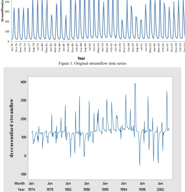
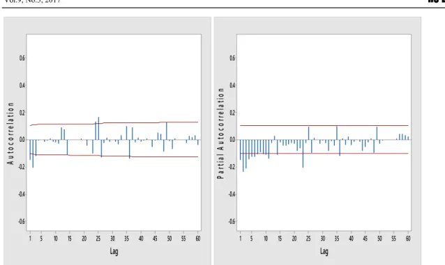
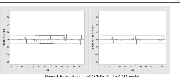
Monthly streamflow data (Fig. 1) indicates seasonal variation having order of 12. To fit the non seasonal ARIMA model, deseasonalization was applied to the streamflow data. The deseasonalization was performed by using STL decomposition method. Deseasonalized monthly streamflow time series (Fig. 2) shows no specific seasonal or trend, but still exhibits non stationary behavior. A non seasonal difference is applied to time series to make it stationary. The plots of ACF, PACF and deseasonalized time series after applying non seasonal difference are shown in Fig. 3. Both plots are examined in order to identify the structure of model. According to the correlations plots, the suggested ARMA model is (1, 3), because PACF plot is suggesting AR(3) term whereas ACF is suggesting MA(1) term. For ARIMA model selection, different ARIMA model structures were estimated to find the best model structure.

Figure 1. Original streamflow time series Year Month 2002 1998 1994 1990 1986 1982 1978 1974 Jan Jan Jan Jan Jan Jan Jan Jan 400 300 200 100 0 -100

de

se

as

on

al

ize

d

st

re

am

flo

w

60 55 50 45 40 35 30 25 20 15 10 5 1 0.6 0.4 0.2 0.0 -0.2 -0.4 -0.6 Lag Au to co rre la tio n 60 55 50 45 40 35 30 25 20 15 10 5 1 0.6 0.4 0.2 0.0 -0.2 -0.4 -0.6 Lag Pa rti al A ut oc or re la tio n

Figure 3. ACF, PACF graphs after non seasonal difference Table 1. AICc and BIC values for different ARIMA model structures

Model Structure AICc BIC

ARIMA(3,1,1) 3777.5 3796.75 ARIMA(0,1,3) 3775.18 3790.6 ARIMA(3,1,3) 3781.3 3808.17 ARIMA(3,1,2) 3779.37 3802.43 ARIMA(3,1,0) 3824.78 3840.2 ARIMA(1,1,1) 3779.37 3790.95 ARIMA(1,1,2) 3776.06 3791.48 ARIMA(1,1,3) 3777.17 3796.41 ARIMA(2,1,1) 3775.47 3790.89 ARIMA(2,1,2) 3777.51 3796.75 ARIMA(2,1,3) 3779.23 3802.29 ARIMA(0,1,2) 3785.13 3796.71

The values of AICc and BIC of the different ARIMA models are shown in Table 5. In this case, the initial

suggested model structure has the minimum AICc and BIC values and has been chosen as best model structure

for deseasonalized streamflow time series. The selected model also passed both tests included in the diagnostic check. The plots of the ACF and PACF for the residuals are shown in Fig. 4, whereas the summary of the Ljung Box test for the deseasonalized ARIMA model is given in Table 2. The results of both tests suggest that the residuals are white noise. From Eq. (1), in back shift notation, the ARIMA(0, 1, 3) model can be written as:

(1-B)d_S

t=(1- Φ1NMA(B)- Φ2NMA(B2)- Φ3NMA(B3))et

(9) By substituting the coefficients, one obtains the model

St- St-1=et+0.3987et-1+0.356et-2+0.183et-3

60 55 50 45 40 35 30 25 20 15 10 5 1 0.6 0.4 0.2 0.0 -0.2 -0.4 -0.6 Lag Au to co rre la tio n 60 55 50 45 40 35 30 25 20 15 10 5 1 0.6 0.4 0.2 0.0 -0.2 -0.4 -0.6 Lag Pa rti al A ut oc or re la tio n

Figure 4. Residual graphs of ACF,PACF of ARIMA model Table 2. Summary of Ljung Box test for deseasonalized ARIMA Model

lag Lag 12 Lag 24 Lag 36 Lag 48

Chi square 1.7626 15.255 41.614 50.408

Df 9 21 33 45

p-value 0.9947 0.8099 0.1445 0.2682

4.2 Evaluation of Best Predicting Model

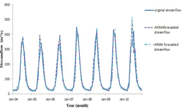
In order to evaluate the performance of the models, one month ahead forecasts were generated for the testing period from January 2004 to December 2010. In Table 3, the both time series models are compared with each other by using statistical indexes. The hydrograph between original forecasted streamflow using ARMA and ARIMA models in Figure 4. On the basis of results of Table 3 and Fig. 5, ARIMA model performs better than ARMA models because ARIMA model gives low value of error and high value of Nash efficiency and also in good fit with the observed data.

Table 3 Evaluation of model performance for testing period on basis of statistical indexes

Statistical Index ARIMA ((0,1,3) ARMA (1,3)

MAPE 17.268 19.642

RMSE 51.525 57.273

Figure 5. Observed and forecasted streamflow hydrograph using ARIMA and ARMA models for testing period

5. Conclusions

In this research, the stochastic nature of streamflow is analyzed with deseasonalized ARIMA and ARMA stochastic models. The ARIMA model has a better performance than ARMA model because it makes time series stationary, in both training and forecasting. The values of mean absolute percentage error and root mean square error of ARIMA model was less than ARMA model. This indicated the superiority of ARIMA models to the ARMA models. it can be concluded that the ARIMA model could be used for forecasting one month ahead streamflow at this site.

References

Adhikary, S. K., Rahman, M., and Gupta, A. D. (2012). A stochastic modelling technique for predicting groundwater table fluctuations with time series analysis. International Journal of Applied Science and Engineering Research1, 238-249.

Ahlert, R., and Mehta, B. (1981). Stochastic analyses and transfer functions for flows of the upper Delaware River. Ecological Modelling14, 59-78.

Ahmad, S., Khan, I. H., and Parida, B. (2001). Performance of stochastic approaches for forecasting river water quality. Water research35, 4261-4266.

Box, G., and Jenkins, G. (1970). (1970). Time series analysis; forecasting and control. Holden-Day, San Francisco(CA).

Box, G. E., and Jenkins, G. M. (1976). Series analysis forecasting and control. Holden-Day, San Francisco, 575. Box, G. E., Jenkins, G. M., and Bacon, D. (1967). "MODELS FOR FORECASTING SEASONAL AND NON-SEASONAL TIME SERIES." DTIC Document.

Box, G. E., Jenkins, G. M., and Reinsel, G. C. (2011). "Time series analysis: forecasting and control," John Wiley & Sons.

Brown, L. C., and Mac Berthouex, P. (2002). "Statistics for environmental engineers," CRC press.

Cleveland, R. B., Cleveland, W. S., McRae, J. E., and Terpenning, I. (1990). STL: A seasonal-trend decomposition procedure based on loess. Journal of Official Statistics6, 3-73.

https://en.wikipedia.org/wiki/Comparison_of_statistical_packages. Accessed 21 November 2015.

Ghafoor, A., and Hanif, S. (2005). Analysis of the trade pattern of Pakistan: Past trends and future prospects.

Gocheva-Ilieva, S. G., Ivanov, A. V., Voynikova, D. S., and Boyadzhiev, D. T. (2014). Time series analysis and forecasting for air pollution in small urban area: an SARIMA and factor analysis approach. Stochastic Environmental Research and Risk Assessment28, 1045-1060.

Hurvich, C. M., and Tsai, C.-L. (1989). Regression and time series model selection in small samples. Biometrika

76, 297-307.

Koutsoyiannis, D. (2000). Generalized mathematical framework for stochastic simulation and forecast of hydrologic time series. Water Resources Research36, 1519-1533.

Kurunç, A., Yürekli, K., and Çevik, O. (2005). Performance of two stochastic approaches for forecasting water quality and streamflow data from Yeşilιrmak River, Turkey. Environmental Modelling & Software20, 1195-1200. Lawrance, A., and Kottegoda, N. (1977). Stochastic modelling of riverflow time series. Journal of the Royal Statistical Society. Series A (General), 1-47.

Lin, J.-Y., Cheng, C.-T., and Chau, K.-W. (2006). Using support vector machines for long-term discharge prediction. Hydrological Sciences Journal51, 599-612.

Ljung, G. M., and Box, G. E. (1978). On a measure of lack of fit in time series models. Biometrika65, 297-303. McCuen, R. H., Knight, Z., and Cutter, A. G. (2006). Evaluation of the Nash–Sutcliffe efficiency index. Journal of Hydrologic Engineering.

Milionis, A., and Davies, T. (1994). Regression and stochastic models for air pollution—I. Review, comments and suggestions. Atmospheric Environment28, 2801-2810.

Modarres, R., and Ouarda, T. (2013). Modelling heteroscedasticty of streamflow times series. Hydrological Sciences Journal58, 54-64.

Reinsel, G., Box, G., and Jenkins, G. (1994). Time Series Analysis: Forecasting and Control. Englewood Cliffs, NJ: Prentice Hall.

Schwarz, G. (1978). Estimating the dimension of a model Ann Stat 6: 461–464. Find this article online.

Tayyab, M., Zhou, J., Zeng, X., and Adnan, R. (2016). Discharge Forecasting By Applying Artificial Neural Networks At The Jinsha River Basin, China. European Scientific Journal12.

Theodosiou, M. (2011). Disaggregation & aggregation of time series components: A hybrid forecasting approach using generalized regression neural networks and the theta method. Neurocomputing74, 896-905.

Valipour, M., Banihabib, M. E., and Behbahani, S. M. R. (2013). Comparison of the ARMA, ARIMA, and the autoregressive artificial neural network models in forecasting the monthly inflow of Dez dam reservoir. Journal of Hydrology476, 433-441.

Yurekli, K., Kurunc, A., and Ozturk, F. (2005). Application of linear stochastic models to monthly flow data of Kelkit Stream. Ecological modelling183, 67-75.

Zhang, G. P. (2003). Time series forecasting using a hybrid ARIMA and neural network model. Neurocomputing