Statistical Network Analysis: Beyond Block Models.

(1)

Statistical Network Analysis: Beyond Block Models

by

Yuan Zhang

A dissertation submitted in partial fulfillment of the requirements for the degree of

Doctor of Philosophy (Statistics)

in the University of Michigan 2016

Doctoral Committee:

Professor Elizaveta Levina, Co-Chair Professor Ji Zhu, Co-Chair

Assistant Professor Ambuj Tewari Professor Mark Newman

(2)

©Yuan Zhang 2016

(3)

A C K N O W L E D G M E N T S

First and foremost, I am indebted to my advisors, Professor Elizaveta Levina and Professor Ji Zhu, for their uncountable guidance and support over the five years of my PhD study, without whom I could not have come so far in my academic career. I am especially grateful for the generous freedom they offered me in pursuing challenges I am enthusiastic about. They set the role models of real scholars and great mentors. I feel very lucky to have them as my advisors.

I thank Professor Ambuj Tewari for being on my preliminary exam and dissertation committee and his warm encouragement, which was espe-cially supportive at the early stage of my research. I thank Professor Yves Atchade for his guidance on improving my teaching and his very kind support for my job applications. I would like to thank Professor Mark Newman for agreeing to be on my dissertation committee.

It has been my privilege to work with my peer PhD students in the Levina-Zhu research group – learning from whom is among the most enjoyable experiences of my PhD life. I thank the wonderful staff in the Department of Statistics at the University of Michigan for their always reliable assistance to my work and study.

I thank Alice Xingwei Lu and Kam Chung Wong for being great friends, without whom it would have been much harder through the difficult times in the past, and I thank all my friends for being the warm company when I am over 11,000 kilometers away from home.

Last but not least, I owe the most to my parents. It has always been so refreshing to recall that they will forever love and be proud of me, no matter I am doing good or bad.

(4)

LIST OF FIGURES

1.1 Political blog networks. Red: conservative; blue: liberal. The pie charts rep-resent the tendency towards each community. The size of the node is

propor-tional to log-degree. . . 3

2.1 Performance of different methods measured by normalized mutual informa-tion as a funcinforma-tion ofr(out-in probability ratio) andµ(feature signal strength). 13 2.2 (a)-(c): the adjacency matrix ordered by different node features; (d) network with nodes colored by continent (taken as ground truth); blue is Africa, red is Asia, green is Europe, cyan is N. America and purple is S. America. (e)-(k) community detection results from different methods; colors are mated to (d) in the best way possible. . . 15

2.3 (a)-(g): adjacency matrix with nodes sorted by features; (h): network with nodes colored by status (blue is partner, red is associate); (i)-(n): community detection results from different methods. . . 17

3.1 Performance of OCCAM measured by exNVI as a function ofCτ. . . 32

3.2 A:(π(1)_{, π}(2)_{, π}(3)_{) = (0.3,}_0.03,_0.03)_{; B:}_(π(1)_{, π}(2)_{, π}(3)_{) = (0.25,}_0.07,_0.04) _{. 34} 4.1 Estimated probability matrices for Graphon 1. . . 47

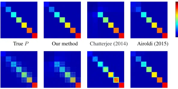
4.2 Estimated probability matrices for Graphon 2. . . 48

4.5 Receiver operating characteristic curve for link prediction on the political blogs network.10%of edges are missing at random. . . 51

A.1 (a) The size of the larger estimated community as a function of the tuning parameterα. (b) Estimation accuracy measured by NMI as a function of the tuning parameter α. Solid lines correspond to JCDC and horizontal dotted lines correspond to spectral clustering, which does not depend onα. . . 56

A.2 MNI between the estimated community structure ˆeand the network commu-nity structurecA (solid lines) and the feature community structurecF (dotted lines). Note that whenn1 =n2 = 60,cA = cF, so the solid and dotted lines coincide. . . 57

C.1 Mean squared error of our method as a function of the constantCin the tuning parameterh=C q logn n . . . 79

(7)

LIST OF TABLES

2.1 Feature coefficientsβˆk estimated by JCDC withw = 5. Best match is

deter-mined by majority vote. . . 14

2.2 Feature coefficientsβˆk, JCDC withwn= 5. . . 16

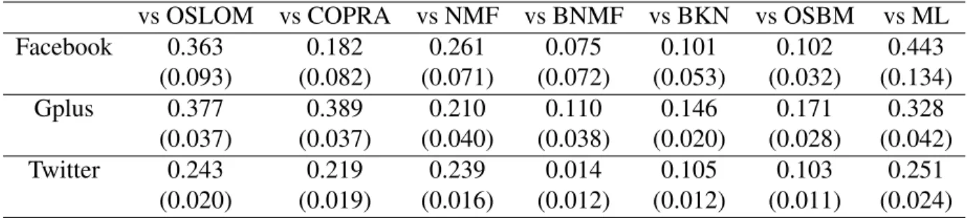
3.1 Mean (SD) of summary statistics for ego-networks . . . 36

3.2 Mean (SD) of exNVI for all methods. . . 36

3.3 Mean (SD) of pairwise differences in exNVI between OCCAM and other methods. . . 36

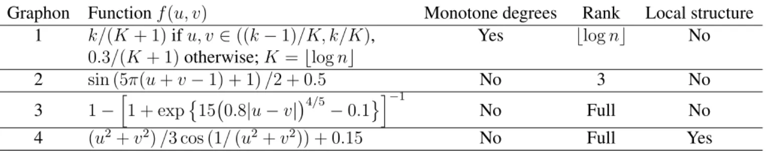
4.1 Synthetic graphons . . . 46

(8)

LIST OF APPENDICES

A Appendix for “Community detection in networks with node features” . . . 55 B Appendix for “Detecting overlapping communities in networks using spectral

methods” . . . 64 C Appendix for “Estimating network edge probabilities by neighborhood

(9)

ABSTRACT

Statistical Network Analysis: Beyond Block Models by

Yuan Zhang

Co-Chairs: Professor Elizaveta Levina and Professor Ji Zhu

Network data represent connections between units of analysis and lead to many inter-esting research questions with diverse applications. In this thesis, we focus on inferring the structure underlying an observed network, which can be thought of as a noisy random real-ization of the unobserved true structure. Different applications focus on different types of underlying structure; one question of broad interest is finding a community structure, with communities typically defined as groups of nodes that share similar connectivity patterns. One common and widely used model for describing a community structure in a network is the stochastic block model. This model has attracted a lot of attention because of its tractable theoretical properties, but it is also well known to oversimplify the structure ob-served in real world networks and often does not fit the data well. Thus there has been a recent push to expand the stochastic block model in various ways to make it closer to what we observe in the real world, and this thesis makes several contributions to this effort.

We first study the problem of detecting communities in the presence of additional node features. Many existing methods detect communities based only on the observed edges be-tween nodes, but in many networks, additional information on node features is available. Recent methods for community detection that incorporate node features typically either depend heavily on correct model specification, which is hard to verify, and/or do not at-tempt to perform feature selection. Including features related to communities can improve community detection, but including unrelated features amounts to adding noise to the data and can lead to substantial reductions in accuracy. In this thesis, we propose a model-free joint criterion for community detection with node features, with the ability to select only relevant features. We show that the underlying new community detection criterion has ap-propriate theoretical performance guarantees and the method is effective on both simulated and real networks.

Another direction we explore in this thesis is modeling and detecting overlapping com-munities. While community detection is commonly formulated as a partition problem, in practice communities in networks tend to overlap. Developing a good model for over-lapping communities has been a challenge, due to identifiability issues and computational costs, although a number of special cases have been addressed. We propose a novel over-lapping model that generalizes the stochastic block model and includes many of the previ-ously studied overlapping models as special cases. The model is flexible and general but maintains identifiability and interpretability of parameters. We propose a fast algorithm to fit this model, establish its consistency, and demonstrate the method outperforms a large number of benchmarks on both simulated and real data examples.

The final contribution of this thesis is a novel method to estimate edge probabilities from a single observed network, a task closely related to the so-called graphon

(10)

estima-tion problem. The stochastic block model is able to infer this underlying edge probabil-ity matrix from a single observation by assuming the underlying probabilprobabil-ity function (the graphon) consists of constant blocks; we deal with the much more general case of piece-wise Lipschitz continuous functions. Our estimator leverages a core technique of classical nonparametric statistics, neighborhood averaging, solving the challenge of defining suit-able neighborhoods on networks. The method is fast and accurate, and adapts to a large range of different graphon families. We also show that it achieves the best theoretical error rate among currently known polynomial time methods for this problem.

(11)

CHAPTER 1

Introduction

This thesis focuses on statistical network analysis. Network-structured data arise in a wide range of areas; examples include social networks, communications, gene regulatory net-works, brain imaging, recommender systems and so on. Analysis of network data plays an important role in many applications, including understanding social structures, disease diagnosis, marketing, and even design of parallel computing algorithms. I investigated several inference problems in statistical network analysis.

Community detection in networks

Communities are groups of nodes that have similar patterns of connection to other nodes. In many networks, nodes from the same community have a higher level of con-nectivity within themselves than average. Communities are present in many real world networks and usually carry meaningful interpretations, corresponding, for example, to real-life social circles, or genes and proteins with similar functions (Resnick et al.,1997;Zhang,

2009;Chamberlain, 1998). My work in this area focused on expanding the capabilities of community detection methods along two directions: utilizing additional node information and detecting overlapping communities.

Community detection using node features

Most existing methods detect communities based only on the observed edges between nodes, but in many networks, additional information on node features is available (Steglich et al.,2006;Snijders et al.,2006;Hummon et al.,1990). The question then arises whether we can combine these two sources of data to improve community detection. Many models that describe the network and the node features jointly have been proposed (Yang et al.,

2013;Xu et al., 2012;Newman and Clauset,2015), but their effectiveness typically relies heavily on correct model specification. Model-free algorithmic methods, such as those proposed byViennet(2012);Binkiewicz et al.(2014) andCheng et al.(2011), are usually based on the simple intuition that nodes in the same community have similar feature (net-work homophily). However, most existing methods ignore the fact that along with node

(12)

features helpful for community detection many datasets include many irrelevant ones, and including nuisance features usually jeopardizes community detection.

In Zhang et al.(2015a), we proposed a novel model-free criterion for community de-tection in weighted networks. To incorporate node features, we model edge weights as Wijz = W(fi, fj;β), where fi is the feature of node i and β is a vector of coefficient

that controls the influence of individual node features on community detection. We al-low different communities to have different βs, and thus some features may be relevant in the formation of some communities but not others, and we learn the weights β from data simultaneously with estimating the community structure. We proved the consistency of our estimator and demonstrated its excellent empirical performance on simulated and data examples. As an example, in a lawyer friendship network (Lazega,2001), our method discovered that type of practice (litigation or corporate), age, and years with the firm are more relevant to the lawyers social circles than gender and the law school from which they graduated.

Overlapping community detection

While community detection is commonly formulated as a partition problem, in practice communities in networks commonly overlap. For example, in a social network people may become friends because they are neighbors, classmates, colleagues, and so on; these are examples of overlapping communities. Developing a good model to describe overlapping communities has long been a challenge, for a number of reasons; in general, it is difficult to disentagle whether a connection between two results from the large number of communities they have in common, or from a higher status of a node that results in higher probability of connections to all the nodes. Most existing models (Airoldi et al.,2008;Latouche et al.,

2009;Ball et al., 2011) address special cases, and even then identifiability is sometimes a challenge. Algorithmic methods (Lancichinetti et al., 2010; Gregory, 2010; Wang et al.,

2011;Gillis and Vavasis, 2014) usually rely on local searches for significant communities and may perform poorly in presence of high degree nodes. The computational cost is another commonly encountered obstacle for many methods in both categories.

(13)

● ● ● ● ● ● ● ● ● ● ● ● ● ● ● ● ● ● ● ● ● ● ● ● ● ● ● ● ● ● ● ● ● ● ● ● ● ● ● ● ● ● ● ● ● ● ● ● ● ● ● ● ● ● ● ● ● ● ● ● ● ● ●●● ● ● ● ● ● ● ● ● ● ● ● ● ●● ● ● ● _● ● ● ● ● ● ● ● ● ● ● ● ● ● ● ● ● ●● ● ● ● ● ● ● ● ● ● ● ● ● ● ● ● ● ● ● ● ● ● ● ● ● ● ● ● ● ● ● ●● ● ● ● ● ● ● ● ● ● ● ● ● ● ● ● ● ● ● ● ● ● ● ● ● ● ● ● ● ● ● ● ● ● ● ● ● ● ● ● ● ● ● ● ● ● ● ● ● ● ● ● ● ● ● ● ● ● _● ●● ● ● ● ● ● ● ● ● ● ● ● ● ● ● ● ● ● ● ● ● ● ● ● ● ● ● ● ● ●_● ● _● ● ● ● ● ● ● ● ● ● ● ● ● ● ● ● ● ● ● ● ● ● ● ● ● ● ● ● ● ● ● ● ● ● ● ● ● ● ● ● ● ●_● ● ● ● ● ● ● ● ● ● ● ● ● ● ● ● _● ● ● ● ● ● ● ● ● _● ● ● ● ●_● ● ● ● ● ● ● ● ● ● ● ● ● ● ● ● ● ●● ● ● ● ● ● ● ● ● ● ● ● ● ● ● ● ● ● ● ● ● ● ● ● ● ● ● ● ● ● ● ● ●● ● ● ● ● ●_● ● ● ● ● ● ● ● ● ● ●

Figure 1.1: Political blog networks. Red: conservative; blue: liberal. The pie charts rep-resent the tendency towards each community. The size of the node is proportional to log-degree.

In Zhang et al.(2014), we proposed a novel overlapping community model, with the goal of keeping it flexible, identifiable, interpretable, and computationally efficient. In our model, each node is mapped to a latent space position and communities correspond to clus-ters in the latent space. We let the nonnegative weighted linear combinations of cluster centers represent overlapping community memberships, with weights corresponding to the degree of association with a particular community. Our model is flexible in that it allows continuous community memberships, so that we can estimate whether a node belongs to a community strongly or weakly. Our model is identifiable under weak conditions and al-lows for heterogeneous node degrees. Our model can be seen as a generalization of several existing overlapping community models, includingLatouche et al. (2009) andKarrer and Newman (2011), and the random dot-product model (Nickel, 2007;Young and Scheiner-man,2007), but none of them have as much flexebility while retaining intepretability. We also designed an efficient algorithm to fit the model, employing a variant of regularized spectral clustering (Von Luxburg, 2007; Qin and Rohe, 2013) to find cluster centers and replacing the commonly usedK-means clustering withK-medians clustering, resulting in an asymptotically unbiased estimator for the overlapping model. Figure1.1shows our esti-mates of overlapping community memberships for the political blog network (Adamic and Glance,2005).

Network edge probability estimation

(14)

ques-tions about the underlying mechanism that generated the network and identifying probable missing or incorrectly recorded links are of interest, and are increasingly drawing the at-tention of statisticians. In this project, we designed a general estimator for network edge probabilities for a network with a more general underlying structure than typical commu-nity models allow.

Aldous(1981) andHoover(1979) showed that in exchangeable networks (those where the order of nodes carries no information), edge probabilities can be represented by

Pij =f(ξi, ξj) (1.0.1)

whereξi ∼ Uniform[0,1]’s andf is a function called the network graphon. The network

adjacency matrixA is then assumed to have independent Bernoulli entries withP(Aij =

1) =Pij the probability of an edge between nodesiandj. Problem (1.0.1) can be viewed

as nonparametric regression with unknown design (Gao et al., 2014), with regularity inP induced by imposing smoothness conditions on f. The difficulty is thatf andξi’s are in

general unidentifiable (Diaconis and Janson,2007) – bit it is still possible, and much more meaningful in practice, to estimate the probability matrixP. In this chapter, we focused on estimatingP under the assumption thatf is piecewise Lipschitz.

Several approaches have been proposed to estimate f and/or P. Step-functions ap-proximations, including Wolfe and Olhede (2013); Olhede and Wolfe (2014); Choi and Wolfe (2014); Choi(2015) and Gao et al.(2014), usually achieve good error rates but re-quire optimization over all possible node partitions, which is NP-hard in principle. The “sort-and-smooth” (SAS) methods such asChan and Airoldi(2014) andYang et al.(2014), focus on graphons with strictly monotone expected node degrees and depend crucially on this rather strong condition. The universal singular value thresholding (USVT) (Chatterjee,

2014), a general matrix completion and denoising tool, can also be used to estimateP with a comparatively loose error bound. Our key insight is that the effectiveness of most meth-ods depends on choosing a good neighborhood for each node, so that averaging overAi0_j0’s fori0 andj0in the neighborhood ofiandjyields a good estimator forPij. The question is

how to define a good neighborhood that both leads to a good error rate and can be learned efficiently.

Our recent paper (Zhang et al., 2015b) proposes a novel neighborhood smoothing method for estimating P with a general structure. We define the neighborhood for each node based on the `2 distance between the “graphon slices” of nodes, represented by the rows of A. This dissimilarity measure is distinct from the distance between the latent ξi’s, and, for example, for networks generated from the stochastic block model, represents

(15)

a more meaningful difference between nodes. We designed an efficient algorithm to se-lect the neighborhood for each node among its neighbors according to the graphon slice distance. Our method is almost tuning-free, numerically robust, computationally efficient, and allows parallelization. We showed that our estimator achieves the best error rate among existing methods that do not rely on optimizing over all node partitions and are thus compu-tationally feasible. Our method can accurately estimate a wide variety of network structures and predict missing edges well when applied to the link prediction problem.

(16)

CHAPTER 2

Community detection in networks with node

features

2.1

Introduction

Community detection is a fundamental problem in network analysis, extensively studied in a number of domains – seeRogers and Kincaid(1981) andSchlitt and Brazma(2007) for some examples of applications. A number of approaches to community detection are based on probabilistic models for networks with communities, such as the stochastic block model

Holland et al. (1983), the degree-corrected stochastic block model Karrer and Newman

(2011), and the latent factor modelHoff (2007). Other approaches work by optimizing a criterion measuring the strength of community structure in some sense, often through spec-tral approximations. Examples include normalized cutsShi and Malik(2000), modularity

Newman and Girvan(2004b); Newman (2006), and many variants of spectral clustering, e.g.,Qin and Rohe(2013).

Many of the existing methods detect communities based only on the network adjacency matrix. However, we often have additional information on the nodes (node features), and sometimes edges as well, for example, Steglich et al. (2006), Snijders et al. (2006) and

Hummon et al. (1990). In many networks the distribution of node features is correlated with community structure McAuley and Leskovec (2012), and thus a natural question is whether we can improve community detection by using the node features. Several gener-ative models for jointly modeling the edges and the features have been proposed, includ-ing the network random effects model Hoff (2003), the embedding feature model Zanghi et al.(2010), the latent variable modelHandcock et al.(2007), the discriminative approach

Yang et al.(2009), the latent multi-group membership graph modelM. Kim(2012), the so-cial circles model for ego networksMcAuley and Leskovec(2012), the communities from edge structure and node attributes (CESNA) modelYang et al.(2013), the Bayesian Graph Clustering (BAGC) modelXu et al. (2012), the topical communities and personal interest

(17)

(TCPI) model Hoang and Lim (2014) and the modified stochastic block model Newman and Clauset(2015). The latter paper was written after this work was completed, and while its goals are somewhat similar to ours by also learning the relationship between the fea-tures and the network from data, it is very different in that it postulates a model connecting them in a particular way. Most of these models are designed for specific feature types, and their effectiveness depends heavily on the correctness of model specification. Model-free approaches include weighted combinations of the network and feature similaritiesViennet

(2012); Binkiewicz et al.(2014), attribute-structure mining Silva et al. (2012), simulated annealing clustering Cheng et al. (2011), and compressive information flow Smith et al.

(2014). Most methods in this category use all the features in the same way without de-termining which ones influence the community structure and which do not, and lack flex-ibility in how to balance the network information with the information coming from its node features, which do not always agree. Including irrelevant node features can only hurt community detection by adding in noise, while selecting features that by themselves cluster strongly may not correspond to features that correlate with the community structure present in the adjacency matrix.

In this chapter, we propose a new joint community detection criterion that uses both the network adjacency matrix and the node features. The idea is that by properly weighing edges according to feature similarities on their end nodes, we strengthen the community structure in the network thus making it easier to detect. Rather than using all available features in the same way, we learn which features are most helpful in identifying the com-munity structure from data. Intuitively, our method looks for an agreement between clusters suggested by two data sources, the adjacency matrix and the node features. Numerical ex-periments on simulated and real networks show that our method performs well compared to methods that use either the network alone or the features alone for clustering, as well as to a number of benchmark joint detection methods.

2.2

The joint community detection criterion

Our method is designed to look for assortative community structure, that is, the type of communities where nodes are more likely to connect to each other if they belong to the same community, and thus there are more edges within communities than between. This is a very common intuitive definition of communities which is incorporated in many commu-nity detection criteria, for example, modularityNewman(2006). Our goal is to use such a community detection criterion based on the adjacency matrix alone, and add feature-based edge weights to improve detection. Several criteria using the adjacency matrix alone are

(18)

available, but having a simple criterion linear in the adjacency matrix makes optimization much more feasible in our particular situation, and we propose a new criterion which turns out to work particularly well for our purposes. Let A denote the adjacency matrix with Aij = 0if there is no edge between nodesiandj, and otherwiseAij >0which can be

ei-ther 1 for unweighted networks or the edge weight for weighted networks. The community detection criterion we start from is a very simple analogue of modularity, to be maximized over all possible label assignmentse:

R(e) = K X k=1 1 |Ek|α X i,j∈Ek Aij . (2.2.1)

Here e is the vector of node labels, with ei = k if node i belongs to community k, for

k = 1, . . . , K, Ek = {i : ei = k}, and |Ek| is the number of nodes in communityk. We

assume each node belongs to exactly one community, and the number of communities K is fixed and known. Rescaling by |Ek|α is designed to rule out trivial solutions that put

all nodes in the same community, and α > 0 is a tuning parameter. Whenα = 2, the criterion is approximately the sum of edge densities within communities, and whenα= 1, the criterion is the sum of average “within community” degrees, which both intuitively represent community structure. This criterion can be shown to be consistent under the stochastic block model by checking the conditions of the general theorem in Bickel and Chen(2009).

The ideal use of features with this criterion would be to use them to up-weigh edges within communities and down-weigh edges between them, thus enhancing the community structure in the observed network and making it easier to detect. However, node features may not be perfectly correlated with community structure, different communities may be driven by different features, as pointed out byMcAuley and Leskovec(2012), and features themselves may be noisy. Thus we need to learn the impact of different features on com-munities as well as balance the roles of the network itself and its features. Letfidenote the

p-dimensional feature vector of nodei. We propose ajoint community detection criterion

(JCDC), R(e, β;wn) = K X k=1 1 |Ek|α X i,j∈Ek AijW(fi, fj, βk;wn) (2.2.2)

whereαis a tuning parameter as in (2.2.1),βk ∈Rpis the coefficient vector that defines the impact of different features on thekth community, andβ :={β1, . . . , βK}. The criterion

is then maximized over bothe andβ. Having a differentβk for eachk allows us to learn

(19)

information fromAandF :={f1, . . . , fn}is controlled bywn, another tuning parameter

which in general may depend onn.

For the sake of simplicity, we model the edge weightW(fi, fj, βk;wn)as a function of

the node featuresfi and fj via a p-dimensional vector of their similarity measures φij =

φ(fi, fj). The choice of similarity measures inφdepends on the type offi(for example, on

whether the features are numerical or categorical) and is determined on a case by case basis; the only important property is thatφassigns higher values to features that are more similar. Note that this trivially allows the inclusion of edge features as well as node features, as long as they are converted to some sort of similarity. To eliminate potential differences in units and scales, we standardize all φij along each feature dimension. Finally, the functionW

should be increasing in hφij, βi, which can be viewed as the “overall similarity” between

nodes, and for optimization purposes it is convenient to take W to be concave. Here we use the exponential function,

wijk=W(fi, fj, βk;wn) =wn−e−hφij,βki (2.2.3)

One can use other functions of similar shapes, for example, the logit exponential function, which we found empirically to perform similarly.

2.3

Estimation

The joint community detection criterion needs to be optimized over both the community assignmentseand the feature parametersβ. Using block coordinate descent, we optimize JCDC by alternately optimizing over the labels with fixed parameters and over the param-eters with fixed labels, and iterating until convergence.

2.3.1

Optimizing over label assignments with fixed weights

When parametersβ are fixed, all edge weightswijk’s can be treated as known constants. It

is infeasible to search over allnK_{possible label assignments, and, like many other}

commu-nity detection methods, we rely on a greedy label switching algorithm to optimize overe, specifically, the tabu searchGlover(1986), which updates the label of one node at a time. Since our criterion involves the number of nodes in each community|Ek|, no easy spectral

approximations are available. Fortunately, our method allows for a simple local approxi-mate update which does not require recalculating the entire criterion. For a given node i

(20)

considered for label switching, the algorithm will assign it to communitykrather thanlif Skk+ 2Si↔k (|Ek|+ 1)α + Sll |El|α > Skk |Ek|α +Sll+ 2Si↔l (|El|+ 1)α , (2.3.1)

where Skk is twice the total edge weights in community k, andSi↔k is the sum of edge

weights between nodeiand all the nodes inEk. When|Ek|and|El|are large, we can ignore

+1in the denominators, and (2.3.1) becomes Si↔k |Ek| ·|Ek| 1−α |El|1−α > Si↔l |El| , (2.3.2)

which allows for a “local” update for the label of node i without calculating the entire criterion. This also highlights the impact of the tuning parameter α: when α = 1, the two sides of (2.3.2) can be viewed as averaged weights of all edges connecting node ito communitiesEk and El, respectively. Then our method assigns node i to the community

with which it has the strongest connection. When α 6= 1, the left hand side of (2.3.2) is multiplied by a factor (|Ek|/|El|)1−α. Suppose |Ek| is larger than |El|; then choosing

0 < α < 1 indicates a preference for assigning a node to the larger community, while α > 1favors smaller communities. A detailed numerical investigation of the role ofα is provided in the Supplemental Material.

The edge weights involved in (2.3.2) depend on the tuning parameterwn. Whenβ = 0,

all weights are equal town−1. On the other hand,wijk ≤wnfor all values ofβ. Therefore,

wn/(wn−1)is the maximum amount by which our method can reweigh an edge. Whenwn

is large,wn/(wn−1)≈1, and thus the information from the network structure dominates.

Whenwnis close to 1, the ratio is large and the feature-driven edge weights have a large

impact. See the Supplemental Material for more details on the choice ofwn.

While the tuning parameterwn controls the amount of influence features can have on

community detection, it does not affect the estimated parametersβ for a fixed community assignment. This is easy to see from rearranging terms in (2.2.2):

R(e, β;wn) = wn K X k=1 1 |Ek|α X i,j∈Ek Aij −g(e, A, β, φ) (2.3.3)

where the functiong does not depend on wn. Note that the term containing wn does not

(21)

2.3.2

Optimizing over weights with fixed label assignments

Since we chose a concave edge weight function (2.2.3), for a given community assignment ethe joint criterion is a concave function ofβk, and it is straightforward to optimize over

βkby gradient ascent. The role ofβk is to control the impact of different features on each

community. One can show by a Taylor-series type expansion around the maximum (details omitted) and also observe empirically that for our method, the estimatedβˆk’s are correlated

with the feature similarities between nodes in community k. In other words, our method tends to produce a large estimatedβˆ_k(`) for a feature with high similarity valuesφ(_ij`)’s for i, j ∈ Ek. However, in the extreme case, the optimalβˆ

(`)

k can be+∞if allφ

(`)

ij ’s are positive

in community k or −∞if all φ(_ij`)’s are negative (recall that similarities are standardized, so this cannot happen in all communities). To avoid these extreme solutions, we subtract a penalty termλkβk1from the criterion (2.2.2) while optimizing overβ. We use a very small value of λ (λ = 10−5 _{everywhere in the chapter) which safeguards against numerically} unstable solutions but has very little effect on other estimated coefficients.

2.4

Consistency

The proposed JCDC criterion (2.2.2) is not model-based, but under certain models it is asymptotically consistent. We consider the setting where the network Aand the features F are generated independently from a stochastic block model and a uniformly bounded distribution, respectively. Let _P(Aij = 1) = ρnPcicj where ρn is a factor controling the

overall edge density andc= (c1, . . . , cn)is the vector of true labels. Assume the following

regularity conditions hold:

1. There exist global constantsMφandMβ, such thatkφijk2 ≤ Mφandkβkk2 ≤ Mβ

for allk, and the tuning parameterwnsatisfieslogwn> MφMβ.

2. LetCk :={i :ci =k}. There exists a global constantπ0 such that|Ck| ≥π0n > 0 for allk.

3. For all1≤k < l≤K,2(K−1)Pkl<min(Pkk, Pll).

Condition 1 states that node feature similarities are uniformly bounded. This is a mild condition in many applications as the node features are often themselves uniformly bounded. In practice, for numerical stability the user may want to standardize node fea-tures and discard individual feafea-tures with very low variance, before calculating the cor-responding similarities φ. Condition 2 guarantees communities do not vanish asymptot-ically. Condition 3 enforces assortativity. Since the estimated labels e are only defined

(22)

up to an arbitrary permutation of communities, we measure the agreement betweeeandc by d(e, c) = minσ∈PK

1

n

Pn

i=11(σ(ei) 6= ci), where PK is the set of all permutations of

{1, . . . , K}.

Theorem 1(Consistency of JCDC). Under conditions1, 2and3, ifnρn → ∞,wnρn →

∞, and the parameterαsatisfies

maxk,l2(K−1)Pkl

mink,l(Pkk, Pll)

≤α ≤1 (2.4.1)

then we have, for any fixedδ >0,

P d arg max e (maxβ R(e, β;wn)), c > δ →0. (2.4.2)

The proof is given in the Supplemental Material.

2.5

Simulation studies

We compare JCDC to three representative benchmark methods which use both the ad-jacency matrix and the node features: CASC (Covariate Assisted Spectral Clustering,

Binkiewicz et al.(2014)), CESNA (Communities from Edge Structure and Node Attributes,

Yang et al. (2013)), and BAGC (BAyesian Graph Clustering, Xu et al. (2012)). In addi-tion, we also include two standard methods that use either the network adjacency alone (SC, spectral clustering on the Laplacian regularized with a small constant τ = 1e −7, as in Amini et al. (2013)), or the node features alone (KM,K-means performed on the p-dimensional node feature vectors, with 10 random initial starting values). We generate networks withn= 150nodes andK = 2communities of sizes100and50from the degree-corrected stochastic block model as follows. The edges are generated independently with probabilityθiθjpif nodesiandjare in the same community, andrθiθjpif nodesiandjare

in different communities. We setp = 0.1and vary rfrom0.25to0.75. We set 5%of the nodes in each community to be “hub” nodes with the degree correction parameterθi = 10,

and for the remaining nodes setθi = 1. All resulting products are thresholded at 0.99 to

ensure there are no probability values over 1. These settings result in the average expected node degree ranging approximately from22to29.

For each node i, we generate p = 2 features, with one “signal” feature related to the community structure and one “noise” feature whose distribution is the same for all nodes. The “signal” feature follows the distributionN(µ,1)for nodes in community 1 and N(−µ,1)for nodes in community 2, with µvarying from0.5to 2(larger µcorresponds

(23)

r µ 0.0 0.5 1.0 1.5 2.0 0.2 0.3 0.4 0.5 0.6 0.7 0.8 0.0 0.2 0.4 0.6 0.8 1.0 r µ 0.0 0.5 1.0 1.5 2.0 0.2 0.3 0.4 0.5 0.6 0.7 0.8 0.0 0.2 0.4 0.6 0.8 1.0 r µ 0.5 1.0 1.5 2.0 0.2 0.3 0.4 0.5 0.6 0.7 0.0 0.2 0.4 0.6 0.8 1.0 r µ 0.0 0.5 1.0 1.5 2.0 0.2 0.3 0.4 0.5 0.6 0.7 0.8 0.0 0.2 0.4 0.6 0.8 1.0 JCDC,w= 5 JCDC,w= 1.5 SC KM r µ 0.0 0.5 1.0 1.5 2.0 0.2 0.3 0.4 0.5 0.6 0.7 0.8 0.0 0.2 0.4 0.6 0.8 1.0 r µ 0.0 0.5 1.0 1.5 2.0 0.2 0.3 0.4 0.5 0.6 0.7 0.8 0.0 0.2 0.4 0.6 0.8 1.0 r µ 0.0 0.5 1.0 1.5 2.0 0.2 0.3 0.4 0.5 0.6 0.7 0.8 0.0 0.2 0.4 0.6 0.8 1.0

CASC CESNA BAGC

Figure 2.1: Performance of different methods measured by normalized mutual information as a function ofr(out-in probability ratio) andµ(feature signal strength).

to stronger signal). For use with CESNA, which only allows categorical node features, we discretize the continuous node features by partitioning the real line into 20 bins using the

0.05,0.1, . . . ,0.95-th quantiles. For the JCDC, based on the study of the tuning parameters in the Supplemental Material, we useα= 1and compare two values ofwn,wn = 1.5and

wn = 5. Finally, agreement between the estimated communities and the true community

labels is measured by normalized mutual information, a measure commonly used in the network literature which ranges between 0 (random guessing) and 1 (perfect agreement). For each configuration, we repeat the experiments 30 times, and record the average NMI over 30 replications.

Figure 2.1 shows the heatmaps of average NMI for all methods under these settings, as a function ofr andµ. As one would expect, the performance of spectral clustering (c), which uses only the network information, is only affected byr(the largerris, the harder the problem), and the performance of K-means (d), which uses only the features, is only affected by µ (the larger µ is, the easier the problem). JCDC is able to take advantage of both network and feature information by estimating the coefficients β from data, and its performance only deteriorates when neither is informative. The informative features are more helpful with a larger value ofw(a), and conversely uninformative features affect perfomance slightly more with a lower value ofw(b), but this effect is not strong. CASC (e) appears to inherit the sharp phase transition from spectral clustering, which forms the basis of CASC; the sharp transition is perhaps due to different community sizes and hub nodes, which are both challenging to spectral clustering; CESNA (f) and BAGC (g) do not

(24)

perform as well overall, with BAGC often clustering all the hub nodes into one community.

2.6

Data applications

2.6.1

The world trade network

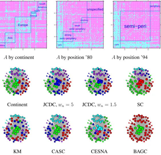
The world trade networkDe Nooy et al.(2011) connects 80 countries based on the amount of trade of metal manufactures between them in 1994, or when not available for that year, in 1993 or 1995. Nodes are countries and edges represent positive amount of import and/or export between the countries. Each country also has three categorical features: the conti-nent (Africa, Asia, Europe, N. America, S. America, and Oceania), the country’s structural position in the world system in 1980 (core, strong semi-periphery, weak semi-periphery, periphery) and in 1994 (core, semi-periphery, periphery). Figures 2.2 (a) to (c) show the adjacency matrix rearranged by sorting the nodes by each of the features. The partition by continent (Figure 2.2(a)) clearly shows community structure, whereas the other two fea-tures show hubs (core status countries trade with everyone), and no assortative community structure. We will thus compare partitions found by all the competing methods to the con-tinents, and omit the three Oceania countries from further analysis because no method is likely to detect such a small community. The two world position variables (’80 and ’94) will be used as features, treated as ordinal variables.

The results for all methods are shown in Figure2.2, along with NMI values comparing the detected partition to the continents. All methods were run with the true valueK = 5. Table 2.1: Feature coefficientsβˆk estimated by JCDC withw = 5. Best match is

deter-mined by majority vote.

Community Best match Position ’80 Position ’94

blue Europe 0.000 0.143

red Asia 0.314 0.127

green Europe 0.017 0.204

cyan N. America 0.107 0.000

purple S. America 0.121 0.000

The result of spectral clustering agrees much better with the continents than that of K-means, indicating that the community structure in the adjacency matrix is closer to the continents that the structure contained in the node features. JCDC obtains the highest NMI value, CASC performs similarly to spectral clustering, whereas CESNA and BAGC both

(25)

20 40 60 20 40 60 Africa Asia Europe North America Oceania South America 20 40 60 20 40 60 core strong semi−periphery weak semi−periphery periphery unspecified 20 40 60 20 40 60 core semi−peri periphery

Aby continent Aby position ’80 Aby position ’94

● ● ● ● ● ● ● ● ● ● ● ● ● ● ● ● ● ● ● ● ● ● ● ● ● ● ● ● Continent JCDC,wn= 5 JCDC,wn= 1.5 SC ● ● ● ● ● ● ● ● ● ● ● ● ● ● ● ● ● ● ● ● ● ● ● ● ● ● ● ●

KM CASC CESNA BAGC

Figure 2.2: (a)-(c): the adjacency matrix ordered by different node features; (d) network with nodes colored by continent (taken as ground truth); blue is Africa, red is Asia, green is Europe, cyan is N. America and purple is S. America. (e)-(k) community detection results from different methods; colors are mated to (d) in the best way possible.

fail to recover the continent partition. Note that no method was able to estimate Africa well, likely due to the disassortative nature of its trade seen in Figure2.2(a). Figure2.2(e) indi-cates that JCDC estimated N. America, S. America and Asia with high accuracy, but split Europe into two communities, since it was run with K = 5and could not pick up Africa due to its disassortative structure. Table2.1contains the estimated feature coefficients, sug-gesting that in 1980 the “world position” had the most influence on the connections formed by Asian countries, whereas in 1994 world position mattered most in Europe.

(26)

2.6.2

The lawyer friendship network

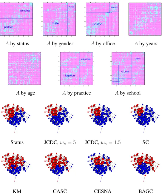
The second dataset we consider is a friendship network of 71 lawyers in a New England corporate law firm Lazega (2001). Seven node features are available: status (partner or associate), gender, office location (Boston, Hartford, or Providence, a very small office with only two non-isolated nodes), years with the firm, age, practice (litigation or corporate) and law school attended (Harvard, Yale, University of Connecticut, or other). Categorical features withM levels are represented byM −1dummy indicator variables. Figures2.3

(a)-(g) show heatmap plots of the adjacency matrix with nodes sorted by each feature, after eliminating six isolated nodes. Partition by status (Figure2.3(a)) shows a strong assortative structure, and so does partition by office (Figure2.3(c)) restricted to Boston and Hartford, but the small Providence office does not have any kind of structure. Thus we chose the status partition as a reference point for comparisons, though other partitions are certainly also meaningful.

Communities estimated by different methods are shown in Figure 2.3 (i)-(o), all run withK = 2. Spectral clustering andK-means have equal and reasonably high NMI values, indicating that both the adjacency matrix and node features contain community informa-tion. JCDC obtains the highest NMI value, with wn = 5 performing slightly better than

wn= 1.5. CASC improves upon spectral clustering by using the feature information, with

NMI just slightly lower than that of JCDC withwn = 1.5. CESNA and BAGC have much

lower NMI values, possibly because of hub nodes, or because they detect communities corresponding to something other than status.

The estimated feature coefficients are shown in Table 2.2. Office location, years with the firm, and age appear to be the features most correlated with the community structure of status, for both partners and associates, which is natural. Practice, school, and gender are less important, though it may be hard to estimate the influence of gender accurately since there are relatively few women in the sample.

Table 2.2: Feature coefficientsβˆk, JCDC withwn = 5.

Comm. gender office years age practice school partner 0.290 0.532 0.212 0.390 0.095 0.000 associate 0.012 0.378 0.725 0.320 0.118 0.097

(27)

10 20 30 40 50 60 10 20 30 40 50 60 partner associate 10 20 30 40 50 60 10 20 30 40 50 60 male female 10 20 30 40 50 60 10 20 30 40 50 60 Boston Providence Hartford

Aby status Aby gender Aby office Aby years

10 20 30 40 50 60 10 20 30 40 50 60 litigation corporate 10 20 30 40 50 60 10 20 30 40 50 60 Harvard/Yale U Conn other

Aby age Aby practice Aby school

● ● ● ● ● ● ● ● ● ● ● ● ● ● ● ● ● ● ● ● ● ● ● ● ● ● ● ● ● ● ● ● ● ● ● ● ● ● ● ● ● ● ● ● Status JCDC,wn= 5 JCDC,wn= 1.5 SC ● ● ● ● ● ● ● ● ● ● ● ● ● ● ● ● ● ● ● ● ● ● ● ● ● ● ● ● ● ● ● ● ● ● ● ● ● ● ● ● ● ● ● ●

KM CASC CESNA BAGC

Figure 2.3: (a)-(g): adjacency matrix with nodes sorted by features; (h): network with nodes colored by status (blue is partner, red is associate); (i)-(n): community detection results from different methods.

(28)

2.7

Discussion

Our method incorporates feature-based weights into a community detection criterion, im-proving detection compared to using just the adjacency matrix or the node features alone, if the cluster structure in the features is related to the community structure in the adjacency matrix. It has the ability to estimate coefficients for each feature within each community and thus learn which features are correlated with the community structure. This ability guards against including noise features which can mislead community detection. The com-munity detection criterion we use is designed for assortative comcom-munity structure, with more connections within communities than between, and benefits the most from using fea-tures that have a similar clustering structure.

This work can be extended in several directions. Variation in node degrees, often mod-eled via the degree-corrected stochastic block model Karrer and Newman (2011) which regards degrees as independent of community structure, may in some cases be correlated with node features, and accounting for degree variation jointly with features can potentially further improve detection. Another useful extension is to overlapping communities. One possible way to do that is to optimize each summand in JCDC (2.2.2) separately and in par-allel, which can create overlaps, but would require careful initialization. Statistical models that specify exactly how features are related to community assignments and edge probabil-ities can also be useful, though empirically we found no such standard models that could compete with the non-model-based JCDC on real data. This suggests that more involved and perhaps data-specific modeling will be necessary to accurately describe real networks, and some of the techniques we proposed, such as community-specific feature coefficients, could be useful in that context.

(29)

CHAPTER 3

Detecting overlapping communities in networks

using spectral methods

3.1

Introduction

The problem of community detection in networks has been actively studied in several dis-tinct fields, including physics, computer science, statistics, and the social sciences. Its applications include understanding social interactions of people (Zachary, 1977;Resnick et al.,1997) and animals (Lusseau et al.,2003), discovering functional regulatory networks of genes (Bolouri and Davidson,2010;Zhang,2009) and even designing parallel comput-ing algorithms (Chamberlain,1998;Hendrickson and Kolda,2000). Community detection is in general a challenging task. The challenges include defining what a community is (commonly taken to be a group of nodes that have more connections to each other than to the rest of the network, although other types of communities are not unusual), formulating realistic and tractable statistical models of networks with communities, and designing fast scalable algorithms for fitting such models.

In this paper, we focus on network models with overlapping communities, with nodes potentially belonging to more than one community at a time. This is common in real-world networks (Palla et al.,2005;Pizzuti,2009), and yet most literature to date has focused on partitioning the network into non-overlapping communities, with some notable exceptions discussed below. Our goal is to design an overlapping community model that is flexible, in-terpretable, and computationally feasible. We will thus focus on models which can be fitted by spectral methods, one of the most scalable tools for fitting non-overlapping community models available to date.

We start with a brief review of relevant work in community detection for non-overlapping communities, which mainly falls into one of two broad categories: algorithmic methods, based on optimizing some criterion reflecting desirable properties of a partition over all

(30)

possible partitions (seeFortunato (2010) for a review), and model fitting, where a genera-tive model with communities is postulated for the network and its parameters are estimated from the observed adjacency matrix (seeGoldenberg et al.(2010) for a review). Perhaps the most popular and best studied generative model for community detection is the stochastic block model (SBM) (Holland and Leinhardt, 1981;Holland et al.,1983). The SBM views the n×n network adjacency matrixA, defined by Aij = 1 if there is an edge between

iandj and 0 otherwise, as a random graph with independent Bernoulli-distributed edges. The Bernoulli probabilities for the edges depend on the node labels ci which take values

in {1, . . . , K}, and the K ×K matrix B containing the probabilities of edges forming between different communities. The node labels can be represented by ann ×K binary community membership matrixZ with exactly one “1” in each row, Zik = 1[ci = k]for

all i, k. Then the probabilities of edges are given by W ≡ _E(A) = ZBZT_{. Thus in}

this model, a node’s label determines its behavior entirely, and thus all nodes in the same community are “stochastically equivalent”, and in particular have the same expected de-gree. This is known to be often violated in practice, due to commonly present “hub” nodes with many more connections than other nodes in their community. The degree-corrected stochastic block model (DCSBM) (Karrer and Newman, 2011) was proposed to address this limitation, which multiplies the probability of an edge between nodes iand j by the product of node-specific positive “degree parameters”θiθj. Both SBM and DCSBM can be

consistently estimated by maximizing the likelihood (Bickel and Chen, 2009;Zhao et al.,

2012), but directly optimizing the likelihood over all label assignments is not computation-ally feasible. A number of faster algorithms for fitting these models have been proposed in recent years, including pseudo-likelihood (Amini et al.,2013), belief propagation (Decelle et al., 2011), spectral approximations to the likelihood (Newman, 2013; Le et al., 2014), spectral clustering on eigenvector ratios to fit DCSBM (Jin, 2015), and generic spectral clustering (Von Luxburg, 2007), used by many and analyzed, for example, in Rohe et al.

(2011) and Sarkar and Bickel (2013). It was further shown that regularization improves on spectral clustering substantially (Amini et al., 2013; Chaudhuri et al., 2012), and its theoretical properties have been further analyzed byQin and Rohe (2013) andJoseph and Yu(2013). While for specific likelihoods one can develop methods that are both fast and more accurate than spectral clustering, such as the pseudo-likelihood (Amini et al., 2013), in general spectral methods remain the most scalable option available.

While the majority of the existing models and algorithms for community detection focus on discovering non-overlapping communities, there has been a growing interest in exploring the overlapping scenario, although both extending the existing models to the overlapping case and developing brand new models remain challenging. Like methods for

(31)

non-overlapping community detection, most existing approaches for detecting overlapping communities can be categorized as either algorithmic or model-based methods. For a com-prehensive review, seeXie et al. (2013). Model-based methods focus on specifying how node community memberships determine edge probabilities. For example, the overlapping stochastic block model (OSBM) (Latouche et al.,2009) extends the SBM by allowing the entries of the membership matrix Z to be independent Bernoulli variables, thus allow-ing multiple “1”s in one row, or all “0”s. The mixed membership stochastic block model (Airoldi et al.,2008) draws membership vectorsZi· from a Dirichlet prior. The

member-ship vector is drawn again to generate every edge, instead of being fixed for the node, so the community membership for nodeivaries depending on which nodejit is interacting with. The “colored edges” model (Ball et al., 2011), sometimes referred to as the Ball-Karrer-Newman model or BKN, allows continuous community membership by relaxing the binary

Z to a matrix with non-negative entries (with some normalization constraints for identifia-bility), and discarding the matrixB. The Bayesian nonnegative matrix factorization model (Psorakis et al.,2011) is related to the model but with notable differences.

Algorithmic methods for overlapping community detection mostly rely on local greedy searches and intuitive criteria. Current approaches include detecting each community sep-arately by maximizing a local measure of goodness of the estimated community ( Lanci-chinetti et al., 2011) and updating an initial estimate of the community membership by neighborhood vote (Gregory,2010). Local methods typically rely heavily on a good start-ing value. Global algorithmic approaches include computstart-ing a non-negative matrix factor-ization approximation to the adjacency matrix and extracting a binary membership matrix from one of the factors (Wang et al.,2011;Gillis and Vavasis,2014). Many heuristic meth-ods do not take heterogeneous node degrees into account, and we found empirically they can perform poorly in the presence of hubs (see Section3.5).

In this chapter, we propose a new generative model for overlapping communities, the overlapping continuous community assignment model (OCCAM). It allows a node to be-long to different communities to a different extent, via the membership vector Zi· with

non-negative entries which represent how strongly a node is associated with various com-munities. We also allow arbitrary degree distributions in a manner similar to the DCSBM, and retain theK×K matrixBwhich allows to interpret connections between communi-ties and compare them. All the model parameters (membership vectors, degree corrections, and community-level connectivity) are identifiable under certain constraints which we will state explicitly. We also develop a fast spectral algorithm to fit OCCAM. Typically, spectral clustering projects the adjacency matrix or its Laplacian onto theK leading eigenvectors representing the nodes’ latent positions, and performsK-means in that lower-dimensional

(32)

space to estimate community memberships. Our key insight here is that when the nodes come from a mixture of clusters (as they would with multiple community memberships), K-means has no chance of recovering the cluster centers correctly; but as long as there are enough pure nodes in each community, K-medians will still be able to identify the clus-ter cenclus-ters correctly by ignoring the “mixed” nodes on the boundaries. We show that our method produces asymptotically consistent parameter estimates as the number of nodes grows as long as there are enough pure nodes and the network is not too sparse. We also employ a simple regularization scheme, since it is by now well known that regularizing spectral clustering substantially improves its performance, especially in sparse networks (Chaudhuri et al., 2012;Amini et al., 2013;Qin and Rohe,2013). We provide an explicit rate for the regularization parameter, implied by our consistency analysis, and show that the overall performance is robust to the choice of the constant multiplier in the regularization parameter as long as the rate is specified correctly.

The rest of the chapter is organized as follows. We introduce the model and discuss parameter identifiability in Section3.2, present the two-stage spectral clustering algorithm in Section 3.3, and state consistency results and describe the choice of the regularization parameter in Section3.4. Some simulation results are presented in Section3.5, where we investigate robustness of our method to the choice of regularization parameter and compare it to a number of benchmark methods for overlapping community detection. We apply the proposed method to a large number of real social ego-networks (networks consisting of all friends of one or several users) from Facebook, Twitter, and GooglePlus in Section 3.6. Section3.7 concludes the chapter with a brief discussion of contributions, limitations, and future work. All proofs are given in the supplemental materials.

3.2

The overlapping continuous community assignment model

3.2.1

The model

Recall that we represent the network by itsn×nadjacency matrixA, a binary symmetric matrix with{Aij, i < j}independent Bernoulli variables andW ≡E(A). We will assume

thatW has the form

W =αnΘZBZTΘ. (3.2.1)

We call this formulation the Overlapping Continuous Community Assignment Model (OC-CAM). The factor αn is a global scaling factor that controls the overall edge probability,

and the only component that depends on n. As is commonly done in the literature, for theoretical analysis we will letαn → 0at a certain rate, otherwise the network becomes

(33)

completely dense asn → ∞. Then×n diagonal matrixΘ = diag(θ1, . . . , θn)contains

non-negative degree correction terms that allow for heterogeneity in the node degrees, in the same fashion as under the DCSBM. We will later assume thatθi’s are generated from

a fixed distributionFΘwhich does not depend on n. Then×K community membership matrixZ is the primary parameter of interest; thei-th rowZi·represents nodei’s

propen-sities towards each of theK communities. We assumeZik ≥0for alli,k, andkZi·k2 = 1 for identifiability. Formally, a node is “pure” if Zik = 1for some k. Later, we will also

assume that the rows Zi·’s are generated independently from a fixed distributionFZ that

does not depend onn. Finally, theK ×K matrix B represents (scaled) probabilities of connections between pure nodes of all communities. Since we are already using αn and Θ, we constrain all diagonal elements ofBto be 1 for identifiability. Other constraints are also needed to make the model fully identifiable; we will discuss them in Section3.2.2.

Note that the general form (3.2.1) can, with additional constraints, incorporate many of the other previously proposed models as special cases. If all nodes are pure andZ has exactly one “1” in each row, we get DCSBM; if we further assume all θi’s are equal, we

have the regular SBM. If the constraint kZi·k2 = 1 is removed and the entries of Z are required to be 0 or 1, and allθi’s are equal, we have the OSBM ofLatouche et al.(2009).

Alternatively, if we set B = I, we have the “colored edges” model ofBall et al. (2011). Our model is also related to the random dot product model (RDPM) (Nickel,2007;Young and Scheinerman,2007), which stipulatesW =X0X0T for some (usually low-rank)X0. This is true for our model ifBis semi-positive definite, since then we can uniquely define

X0 =

√

αnΘZB1/2. OCCAM is thus more general than all of these models, and yet is

fully identifiable and interpretable.

3.2.2

Identifiability

The parameters in (3.2.1) obviously need to be constrained to guarantee identifiability of the model. All models with communities, including the SBM, are considered identifiable if they are identifiable up to a permutation of community labels. To show the interplay between the model parameters, we first state identifiability conditions treating all ofαn,Θ,

Z, and Bas constant parameters, and then discuss what happens if ΘandZ are treated as random variables as we do in the asymptotic analysis. The following conditions are sufficient for identifiability:

I1 Bis full rank and strictly positive definite, withBkk= 1for allk.

I2 AllZik ≥ 0, kZi·k2 = 1 for all i = 1, . . . , n, and there is at least one “pure” node in every community, i.e., for eachk = 1, . . . , K, there exists at least oneisuch that

(34)

Zik = 1.

I3 The degree parametersθ1, . . . , θnare all positive andn−1

Pn

i=1θi = 1.

Theorem 2. If conditions(I1), (I2)and(I3)hold, the model is identifiable, i.e., if a given

probability matrix W corresponds to a set of parameters(αn,Θ,Z,B)through (3.2.1),

these parameters are unique up to a permutation of community labels.

The proof of Theorem 2 is given in the supplemental materials. In general, identifi-ability is non-trivial to establish for most overlapping community models, since, roughly speaking, an edge between two nodes can be explained by either their common member-ships in many of the same communities, or the high probability of edges between their two different communities, a problem that does not occur in the non-overlapping case. Among previously proposed models, the OSBM was shown to be identifiable (Latouche et al., 2009), but their argument does not extend to our model since they only considered

Z with binary entries. The identifiability of the BKN model was not discussed by Ball et al.(2011), but it is relatively straightforward (though still non-trivial) to show that it is identifiable as long as there are pure nodes in each community.

While Theorem2makes the model in (3.2.1) well defined, it is also common practice in the community detection literature to treat some of the model components as random quantities. For example, Holland et al. (1983) treat community labels under the SBM as sampled from a multinomial distribution, andZhao et al. (2012) treat the degree parame-tersθi’s in DCSBM as sampled from a general discrete distribution. For our consistency

analysis, treatingθi’s andZi·’s as random significantly simplifies conditions and allows for

an explicit choice of rate for the tuning parameterτn, which will be defined in Section3.3.

We will thus treat ΘandZ as random and independent of each other for the purpose of theory, assuming that the rows ofZ are independently generated from a distribution FZ

on the unit sphere, andθi’s are i.i.d. from a distributionFΘ on positive real numbers. The conditionsI2andI3are then replaced with the following two conditions, respectively:

RI2 FZ = πpFp +πoFo is a mixture of a multinomial distribution Fp on K categories

for pure nodes and an arbitrary distributionFo on{z ∈RK :zk≥0,kzk2 = 1}for nodes in the overlaps, andπp >0.

RI3 FΘis a probability distribution on(0,∞)satisfying R∞

0 t dFΘ(t) = 1.

The distribution Fo can in principle be any distribution on the positive quadrant of

the unit sphere. For example, one could first specify that with probabilityπk1,...,km, node

(35)

Alternatively, one could generate values for the m non-zero entries of Zi· from an

m-dimensional Dirichlet distribution, and set the rest to 0.

Here we emphasize that the conditions guaranteeing identifiability is an indispensable part of our model. Ideas similar to (3.2.1) previously appeared in the literature, see, for example, Appendix C ofBall et al.(2011). However, without proper identifiability condi-tions, the parameters are not meaningful.

3.3

A spectral algorithm for fitting the model

The primary goal of fitting this model is to estimate the membership matrix Z from the observed adjacency matrix A, although other parameters may also be of interest. Since computational scalability is one of our goals, we focus on algorithms based on spectral de-compositions, one of the most scalable approaches available. Recall that spectral clustering typically works by first representing all data points (thennodes) by ann×KmatrixX con-sisting of leading eigenvectors of a matrix derived from the data, which we callGfor now, and then applyingK-means clustering to the rows ofX. For example, under the SBM, the matrixGshould be chosen to have eigenvectorsX that approximate the eigenvectorsX0 ofW =_E(A)as closely as possible, since the eigenvectors ofW are piecewise constant and contain all the community information. A naive choiceG = Ais intuitively appeal-ing, though it has been shown in practice and in theory (Sarkar and Bickel,2013) that the graph Laplacian ofA, i.e.,L=D−1/2_AD−1/2_{, where}_D ₌_diag₍_A₁₎_{, is a better choice,} or, for sparse graphs, different regularized versions of L (Amini et al., 2013; Chaudhuri et al.,2012;Qin and Rohe,2013;Joseph and Yu,2013). An additional step of normalizing the rows ofX before performingK-means is often appropriate if the underlying model is assumed to be the degree-corrected stochastic blockmodel (Qin and Rohe,2013).

Regardless of the matrix chosen to estimate the eigenvectors ofW, the key difference between the regular SBM under which spectral clustering is usually studied and our model is that under the SBM there are only K unique rows in X0, and thus K-means can be expected to accurately cluster the rows of X, which is a noisy version of X0. Under our model, the rows of X0 are linear combinations of the “pure” rows corresponding to “centers” of the K communities. Thus even if we could recover X0 exactly, K-means is not expected to work, and it is in fact straightforward to show that theK-means algorithm does not recover the positions of pure nodes correctly unless non-pure nodes either vanish in proportion or converge to pure nodes’ latent positions asn grows (proof omitted here as it is not needed for our main argument). The key idea of our algorithm is to replace K-means withK-medians clustering: if the proportion of pure nodes is not too low, then

(36)

the latent positions of the cluster centers can still be recovered correctly, and therefore the coefficients of mixed nodes can be estimated accurately by projecting onto the pure nodes. Other details of the algorithm involve regularization and normalization that are necessary for dealing with sparse networks and heterogeneous degrees.

Our algorithm for fitting the OCCAM takes as input the adjacency matrix A and a regularization parameterτn>0which we use to regularize the estimated latent node

posi-tions directly. This is easier to handle technically than regularizing the Laplacian, and we will give an explicit rate forτnthat guarantees asymptotic consistency in Section3.4. The

algorithm proceeds as follows:

1. Compute UÂLÂUÂT, where LÂ is the K × K diagonal matrix containing the K

leading eigenvalues ofA, andUˆAis then×K matrix containing the corresponding

eigenvectors. While the true W = _E(A) is positive definite, in practice some of the eigenvalues ofAmay be negative; if that happens, we truncate them to 0. Let

ˆ

X ≡UˆALˆ

1/2

A be the estimated latent node positions.

2. Compute Xˆ∗, a normalized and regularized version of Xˆ, the rows of which are given byXˆ_i∗_·= 1

kXˆi·k2+τn

ˆ

Xi·.

3. Perform K-medians clustering on the rows of Xˆ∗ and obtain K estimated cluster centerss1, . . . ,sK ∈RK, i.e., {s1, . . . ,sK}= arg min s1,...,sK 1 n n X i=1 min s∈{s1,...,sK} ˆ X_i∗_·−s 2 (3.3.1)

Form theK×KmatrixSˆwith rows equal to the estimated cluster centerssˆ1, . . . ,sK.

4. Project the rows ofXˆ∗ onto the span ofs1, . . . ,sK, i.e., compute the matrixXˆ∗Sˆ−1

and normalize its rows to have norm 1 to obtain the estimated community member-ship matrixZˆ.

This algorithm can also be used to obtain other types of community assignments. For example, to obtain binary rather than continuous community membership, we can threshold each element of Zˆ to obtain Zˆ0

ik = 1( ˆZik > δK)(see Section 3.5 and Section3.6). To

(37)

3.4

Asymptotic consistency

3.4.1

Main result

In this section, we show consistency of our algorithm for fitting the OCCAM as the num-ber of nodes n and possibly the number of communities K increase. For the theoretical analysis, we treatZ andΘ as random variables, as was done byZhao et al. (2012). We first state regularity conditions on the model parameters.

A1 The distributionFΘis supported on(0, Mθ), and for allδ >0satisfiesδ−1

Rδ

0 dFΘ(t)≤ Cθ, whereMθ >0andCθ >0are global constants.

A2 Letλ0 andλ1 be the smallest and the largest eigenvalues of E[θi2ZiT·Zi·B],

respec-tively. Then there exist global constantsMλ0 >0andMλ1 >0such thatKλ0 ≥Mλ0

andλ1 ≤Mλ1.

A3 There exists a global constantmB >0such thatλmin(B)≥mB.

A key ingredient of our algorithm is the K-medians clustering, and consistency of K-medians requires its own conditions on clusters being well separated in the appropriate metric. Thesampleloss function forK-medians is defined by

Ln(Q;S) = 1 n n X i=1 min 1≤k≤KkQi·−Sk·k2

whereQ∈ _Rn×K _{is a matrix whose rows} _Q

i·are vectors to be clustered, andS ∈RK×K is a matrix whose rowsSk·are cluster centers.

Assuming the rows of Qare i.i.d. random vectors sampled from a distributionG, we similarly define thepopulationloss function forK-medians by

L(G;S) =

Z

min

1≤k≤Kkx−Sk·k2dG.

Finally we define the Hausdorff distance, which is used here to measure the dissimilarity between two sets of cluster centers. Specifically, for S,T ∈ _RK×K_{, let} _D

H(S,T) =

minσmaxkkSk·−Tσ(k)·k2, whereσranges over all permutations of{1, . . . , K}.

DefineXi·=θiZi·B1/2 andX_i∗·=kXi·k₂−1Xi·=kZi·B1/2k−₂1Zi·B1/2, a