Exploring the semantic content of unsupervised graph embeddings : an empirical study.

Deposited in DRO:

12 July 2019

Version of attached le:

Published Version

Peer-review status of attached le:

Peer-reviewed

Citation for published item:

Bonner, Stephen and Kureshi, Ibad and Brennan, John and Theodoropoulos, Georgios and McGough, Stephen and Obara, Boguslaw (2019) 'Exploring the semantic content of unsupervised graph embeddings : an empirical study.', Data science and engineering., 4 (3). pp. 269-289.

Further information on publisher's website:

https://doi.org/10.1007/s41019-019-0097-5

Publisher's copyright statement: c

The Author(s) 2019. This article is distributed under the terms of the Creative Commons Attribution 4.0

International License (http://creativecommons.org/licenses/by/4.0/), which permits unrestricted use, distribution, and reproduction in any medium, provided you give appropriate credit to the original author(s) and the source, provide a link to the Creative Commons license, and indicate if changes were made.

Use policy

The full-text may be used and/or reproduced, and given to third parties in any format or medium, without prior permission or charge, for personal research or study, educational, or not-for-prot purposes provided that:

• a full bibliographic reference is made to the original source • alinkis made to the metadata record in DRO

• the full-text is not changed in any way

The full-text must not be sold in any format or medium without the formal permission of the copyright holders. Please consult thefull DRO policyfor further details.

https://doi.org/10.1007/s41019-019-0097-5

Exploring the Semantic Content of Unsupervised Graph Embeddings:

An Empirical Study

Stephen Bonner1 _{· Ibad Kureshi}2 _{· John Brennan}1 _{· Georgios Theodoropoulos}3 _{· Andrew Stephen McGough}4 _·

Boguslaw Obara1

Received: 12 March 2018 / Revised: 23 May 2019 / Accepted: 22 June 2019 © The Author(s) 2019

Abstract

Graph embeddings have become a key and widely used technique within the field of graph mining, proving to be successful across a broad range of domains including social, citation, transportation and biological. Unsupervised graph embedding techniques aim to automatically create a low-dimensional representation of a given graph, which captures key structural elements in the resulting embedding space. However, to date, there has been little work exploring exactly which topological structures are being learned in the embeddings, which could be a possible way to bring interpretability to the process. In this paper, we investigate if graph embeddings are approximating something analogous to traditional vertex-level graph features. If such a relationship can be found, it could be used to provide a theoretical insight into how graph embedding approaches function. We perform this investigation by predicting known topological features, using supervised and unsupervised meth-ods, directly from the embedding space. If a mapping between the embeddings and topological features can be found, then we argue that the structural information encapsulated by the features is represented in the embedding space. To explore this, we present extensive experimental evaluation with five state-of-the-art unsupervised graph embedding techniques, across a range of empirical graph datasets, measuring a selection of topological features. We demonstrate that several topological features are indeed being approximated in the embedding space, allowing key insight into how graph embeddings create good representations.

Keywords Graph embeddings · Neural networks · Representation learning

1 Introduction

Representing the complex and inherent links and relation-ships between and within datasets in the form of a graph is a widely performed practice across many scientific disciplines [1]. One reason for the popularity is that the structure or topology of the resulting graph can reveal important and

unique insights into the data it represents. Recently, ana-lysing and making predictions about graph using machine learning has shown significant advances in a range of com-monly performed tasks over traditional approaches [2]. Such tasks include predicting the formation of new edges within the graph and the classification of vertices [3]. However, graphs are inherently complex structures and do not natu-rally lend themselves as input into existing machine learning methods, most of which operate on vectors of real numbers.

Graph embeddings1_{are a family of machine learning}

models which learn latent representations for the vertices within a graph. The goal of all graph embedding techniques is broadly the same: to transform a complex graph, with no inherent representation in vector space, into a low-dimen-sional vector (often in the range of 50–300) representation of the graph or its elements. More concretely, the objective of a graph embedding technique is to learn some function

* Stephen Bonner

[email protected] Boguslaw Obara

[email protected]

1 _{Department of Computer Science, Durham University,}

Durham, UK

2 _{InlecomSystems, Brussels, Belgium}

3 _{School of Computer Science and Engineering, SUSTech,}

Shenzhen, China

4 _{School of Computing, Newcastle University, Newcastle, UK}

1 _{In this work, we focus on vertex representation learning}

f ∶V →ℝd which is a mapping from the set of verticesV to a set of embeddings for the vertices, where d is the required dimensionality of the resulting embedding. This results in the mapping function f producing a matrix of dimensions |V| by d, i.e. an embedding of size d for each vertex in the graph. It should be noted that this mapping is intended to capture the latent structure from a graph by mapping similar vertices together in the embedding space. Many of the recent approaches are able to produce low-dimensional graph rep-resentations without the need for labelled datasets. These representations can then be utilised as input to secondary supervised models for downstream prediction tasks, includ-ing classification [4] or link prediction [5]. Thus, unsuper-vised graph embeddings are becoming a key area of research as they act as a translation layer between the raw graph and some desired machine learning model.

However, to date, there has been little research performed into why graph embedding approaches have been so success-ful. They all aim to capture as much topological information as possible during the embedding process, but how this is achieved, or even exactly what structure is being captured, is currently not known. In this work, we focus solely upon unsupervised graph embedding techniques as we want to explore what features the techniques learn from the topol-ogy alone, without the requirement for labels. In previous work [6], we provided a framework which could be used to directly measure the ability of graph embeddings to capture a good representation of a graph’s topology. In this paper, we expand upon this work by attempting to provide insight into the graph embedding process itself. We attempt to explore if the known and mathematically understood range of topo-logical features [1] is being approximated in the embedding space. To achieve this, we investigate if a mapping from the embedding space to a range of topological features is pos-sible. We hypothesise that if such a mapping can be found, then the topological structure represented by that feature is thus approximately captured in the embedding space. Such a discovery could start to provide a theoretical framework for the use of graph embeddings, by experimentally demonstrat-ing which topological structures are approximated to create the representations.

Our methodology employs a combination of supervised and unsupervised models to predict topological features directly from the embeddings. The features we are inves-tigating first go through a pre-processing step to transform them into discrete classes to enable classification. We make the following contributions whilst exploring this area: – We investigate if unsupervised graph embeddings are

learning something analogous with traditional vertex-level graph features. If this is the case, is there a par-ticular type of feature which is being approximated most frequently?

– We empirically show, to the best of our knowledge for the first time, that several known topological features are present in graph embeddings. This can be used to help bring interpretability to the graph embedding process by detailing which graph features are key in creating high-quality representations.

– We provide detailed experimental evidence, with five state-of-the-art unsupervised graph embedding approaches, across seven topological features and six empirical graph datasets to support our claims.

Reproducibility—we make all experiments performed in this paper reproducible by open-sourcing our code,2 _reporting

key model hyper-parameters and presenting results on public benchmark graph datasets.

In Sect. 2 we explore prior work. In Sect. 3 we detail our approach for providing an experimental methodology for assessing known topological features approximated by graph embeddings; Sect. 4 details the experiment set-up. In Sect. 5 we present our results, and in Sect. 6 we conclude this paper along with suggestions for further expansions of this work.

1.1 Notation

We adopt here the commonly used notation for represent-ing a graph or network3_{G= (V,E) as an undirected graph}

which comprises a finite set of vertices (sometimes referred to as nodes)V and a finite set of edges E. The elements of

E are an unordered tuple {u,v} of vertices u,v∈V . Here G

could be a graph-based representation of a social, citation or biological network [7]. The adjacency matrix 𝐀= (a_i,j)

for a graph is symmetric matrix of size |V| by |V|, where

(a_i,j) is 1 if an edge is present between vertices i and j or

0 otherwise.

2 Previous Work

This section explores the prior research regarding graph embedding techniques and previous approaches measur-ing known features in embeddmeasur-ings. We first introduce the notation of graph embeddings, detail supervised and factor-isation-based approaches, explore in detail state-of-the-art unsupervised approaches which will be used throughout the rest of the paper and finally review past attempts to provide interpretability to embedding approaches.

2 _{https ://githu b.com/sbonn er0/unsup ervis ed-graph -embed ding/.} 3 _{To avoid confusion with neural networks we will use the term}

graph throughout the remainder of the paper without loss of general-ity.

2.1 Introduction to Graph Embeddings

The ability to automatically learn some descriptive numer-ical-based representation for a given graph is an attractive goal and could provide a timely solution to some com-mon problem within the field of graph mining. Traditional approaches have relied upon extracting features—such as various measures of a vertex’s centrality [8]—capturing the required information about a graph’s topology, which could then be used in some downstream prediction task [9–12]. However, such a feature extraction-based approach relies solely upon the handcrafted features being a good represen-tation of the target graph. Often a user must use extensive domain knowledge to select the correct features for a given task, with a change in task often requiring the selection of new features [9].

Graph embedding models are a collection of machine learning techniques which attempt to learn key features from a graph’s topology automatically, in either a super-vised or unsupersuper-vised manner, removing the often cumber-some task of end-users manually selecting representative graph features [4]. This process, known as feature selection [13] in the machine learning literature, has clear disadvan-tages as certain features may only be useful for a certain task. It could even negatively affect model performance if utilised in a task for which they are not well suited. Argu-ably, many of the recent exciting advances seen in the field of deep learning have been driven by the removal of this feature selection process [5], instead of allowing models to learn the best data representations themselves [14]. For a selection of recent review papers covering the complete fam-ily of graph embedding techniques, readers are referred to [15–18]. The work presented in this paper focuses on neural network-based approaches for graph embedding (as these have demonstrated superior performance compared with traditional approaches [2]).

The study of neural networks (NNs) is a field within machine learning inspired by the brain [14]. NNs model problems via the use of connected layers of artificial neu-rons, where each network has an input layer, at least one hid-den layer and an output layer. The activation of each neuron in a layer is given by a pre-specified function, with each ron taking a weighted sum of all the outputs of those neu-rons which feed into it. These weights are learned through training examples which are fed through the network, with modifications made to the weights via back-propagation to increase the probability of the NN producing the desired result [14].

2.1.1 Supervised Approaches

Within the field of machine learning, approaches which are supervised are perhaps the most studied and understood

[14]. In supervised learning, the datasets contain labels which help guide the model in the learning process. In the field of graph analysis, these labels are often present at the vertex level and contain, for example, the metadata of a user in a social network.

Perhaps the largest area of supervised graph embeddings is that of graph convolutional neural networks (GCNs) [19], both spectral [20, 21] and spatial [22] approaches. Such approaches pass a sliding window filter over a graph, in a manner analogous with convolutional neural networks from the computer vision field [14], but with the neighbourhood of a vertex replacing the sliding window. Current GCN approaches are supervised and thus require labels upon the vertices. This requirement has two significant disadvantages: Firstly, it limits the available graph data which can be used due to the requirement for labelled vertices. Secondly, it means that the resulting embeddings are specialised for one specific task and cannot be generalised for a different prob-lem without costly retraining of the model for the new task. 2.1.2 Factorisation Approaches

Before the recent interest in learning graph embeddings via the use of neural networks, a variety of other approaches were explored. Often these approaches took the form of matrix factorisation, in a similar vein to classical dimen-sionality reduction techniques such as principal competent analysis (PCA) [15, 23]. Such approaches first calculate the pairwise similarity between the vertices of a graph and then find a mapping to a lower-dimensional space such that the relationships observed in the higher dimensions are pre-served. An early example of such an approach is that of the Laplacian eigenmaps, which attempts to directly fac-torise the Laplacian matrix of a given graph [24]. Other approaches, often using the adjacency matrix, define the relationship in low-dimensional space between two verti-ces in the graph as being determined by the dot-product of their corresponding embeddings. Such approaches include graph factorisation [25], GraGrep [26] and HOPE [27]. Such dimensionality reduction-based approaches are often quad-ratic in complexity [17], and the predictive performance of the embeddings has largely been superseded by the recent neural network-based methods [2].

2.2 Unsupervised Stochastic Embeddings

DeepWalk [4] and Node2Vec [5] are the two main approaches for random walk-based embedding. Both of these approaches borrow key ideas from a technique enti-tled Word2Vec [28] designed to embed words, taken from a sentence, into vector space. The Word2Vec model is able to learn an embedding for a word by using surrounding words within a sentence as targets for a single hidden layer

neural network model to predict. Due to the nature of this technique, words which co-occur together frequently in sen-tences will have positions which are close within the embed-ding space. The approach of using a target word to predict neighbouring words is entitled Skip-Gram and has been shown to be very effective for language modelling tasks [29]. 2.2.1 DeepWalk

The key insight of DeepWalk is to use random walks upon the graph, starting from each vertex, as the direct replace-ment for the sentences required by Word2Vec. A random walk can be defined as a traversal of the graph rooted at a vertex v_t∈V , where the next step in the walk is chosen

uniformly at random from the vertices incident upon v_t [30];

these walks are recorded as wt₀,…,wt

n (where t is the walk

starting from vt of length n, and wti∈V ), i.e. a sequence

of the vertices visited along the random walk starting from

v_t=wt

0 . DeepWalk is able to learn unsupervised

representa-tions of vertices by maximising the average log probability

𝐏 over the set of vertices V:

where c is the size of the training context of vertex wt n.4

The basic form of Skip-Gram used by DeepWalk defines the conditional probability 𝐏(wt

i+j|w t

i) of observing a nearby

vertex wt_i+j , given the vertex wt_i from the random walk t, can

be defined via the softmax function over the dot-product between their features [4]:

where 𝐖_wt i and

𝐖� wt

i+j are the hidden layer and output layer

weights of the Skip-Gram neural network, respectively. 2.2.2 Node2Vec

Whilst DeepWalk uses a uniform random transition prob-ability to move from a vertex to one of its neighbours, Node-2Vec biases the random walks. This biasing introduces two user-controllable parameters which dictate how far from, or close to, the source vertex the walk progresses. This is done to capture either the vertex’s role in its local neighbourhood (homophily), or alternatively, its role in the global graph (1) 1 |V| |V| ∑ t=1 n ∑ i=0 ∑ −c≤j≤c,j≠0 log𝐏(wt_i+j|wt_i), (2) 𝐏(wt_i+j�wt_i) = exp(𝐖⊺ wt i 𝐖� wt i+j ) ∑�V� t=1exp(𝐖 ⊺ wt i 𝐖� vt) ,

structure (structural equivalence) [5]. Changing the random walk means that Node2Vec has a higher accuracy over Deep-Walk for a selection of vertex classification problems [5].

2.3 Unsupervised Hyperbolic Embeddings

Recently, a new family of graph embedding approaches has been introduced, which embed vertices into hyperbolic, rather than Euclidean space [31, 32]. Hyperbolic space has long been used to analyse graphs which exhibit high levels of hierarchical or community structure [33], but it also has prop-erties which could make it an interesting space for embed-dings [32]. Hyperbolic space can be considered ‘larger’ than Euclidean with the same number of dimensions; as the space is curved, its total area grows exponentially with the radius [32]. For graph embeddings, this key property means that one effectively has a much larger range of possible points into which the vertices can be embedded. This property allows for closely correlated vertices to be embedded close together, whilst also maintaining more distance between disparate ver-tices, resulting in an embedding which has the potential to capture more of the latent community structure of a graph.

The hyperbolic approach we focus on was introduced by Chamberlain [32] and uses the Poincaré disc model of 2D hyperbolic space [34]. In their model, the authors use polar coordinates x= (r,𝜃) , where r∈ [0, 1] and 𝜃∈ [0, 2𝜋] to

describe a point in space for each vertex v in the Poincaré disc, which allows for the technique to be significantly sim-plified [32]. Similar to DeepWalk, an inner-product is used to define the similarity between two points within the space. The inner-product of two vectors in a Poincaré disc can be defined as follows [32]:

where x= (rx,𝜃x) and y= (ry,𝜃y) are the two input vectors

representing two vertices and arctanh is the inverse hyper-bolic tangent function [32].

To create their hyperbolic graph embedding, the authors use the softmax function of Eq. 2, common with DeepWalk and others, but importantly replacing the Euclidean inner-products with the hyperbolic inner-inner-products of Eq. 3. Aside from this, hyperbolic approaches share many similarities with the stochastic approaches with regard to their input data and training procedure. For example, the hyperbolic approaches are still trained upon pairs of vertex IDs, taken from sequences of vertices generated via random walks on graphs.

2.4 Unsupervised Auto‑encoder‑Based Approaches

There is an alternative set of approaches for graph embed-dings which do not rely upon random walks. Instead of

(3)

<_x,y>=_||x_||||y_||cos(𝜃_x−𝜃_y),

(4)

=4 arctanhr_xarctanhr_y cos(𝜃_x−𝜃_y),

4 _{Note if i}+_j<0 then we skip these from the sum as we are past the

adapting a technique based upon capturing the meaning of language, such models are designed specifically for cre-ating graph embeddings using deep learning [14]—deep auto-encoders [35]. Auto-encoders are an unsupervised neural network, where the goal is to accurately reconstruct the input data through explicit encoder and decoder stages [36]. Two such approaches are structural deep network embedding (SDNE) [37] and deep neural networks for learning graph representations (DNGR) [38].

The authors of these approaches argue that a deep neu-ral network, versus the shallow Skip-Gram model used by both DeepWalk and Node2Vec, is much more capable of capturing the complex structure of graphs. In addition, the authors argue that for a successful embedding, it must capture both the first- and second-order proximity of ver-tices. Here the first-order proximity measures the similar-ity of the vertices which are directly incident upon one another, whereas the second-order proximity measures the similarity of vertices neighbourhoods. To capture both of these elements SDNE has a dual-objective loss function for the model to optimise. The input data to SDNE are the adjacency matrix 𝐀 , where each row a represents the

neighbourhood of a vertex.

The objective function for SDNE comprises two distinct terms: The first term captures the second-order proximity of the vertices neighbourhood, whilst the second captures the first-order proximity of the vertices by iterating over the set of edges E:

where qi and q′i are the input and reconstructed

representa-tion of the input, ⊙ is the element-wise Hadamard product,

and b_i is a scaling factor to penalise the technique if it

pre-dicts zero too frequently, w(k) is the weight of the kth layer

in the auto-encoder technique, and 𝛼 is a user-controllable

parameter defining the importance of the second term in the final loss score [37].

To initialise the weights of the deep auto-encoder used for this approach, an additional neural network must be trained to find a good starting region for the parameters. This pre-training neural network is called a deep belief network and is widely used within the literature to form the initialisation step of deeper models [39]. However, this pre-training step is not required by either the stochastic or hyperbolic approaches as random initialisation is used for the weights and adds significant complexity.

In comparison with SDNE, instead of relying solely upon the raw adjacency matrix as input, DNGR creates a new denser representation to be passed to an auto-encoder [38]. The authors have the model reconstruct the pointwise mutual information matrix (PPMI) of the input graph, which (5) LSDNE= |V| ∑ i=1 ||(q�_i−qi)⊙bi||22+𝛼 |E| ∑ u,v=1 au,v||(w(uk)−w (k) v )|| 2 2,

captures vertex co-occurrence information in a sequence created via a random surfer model. Additionally, instead of passing this to a traditional auto-encoder, a stacked de-noising auto-encoder is used with the goal of creating a more robust vertex representation. This stacked de-noising auto-encoder adds a small quantity of noise to the input data, which the model must learn to disregard during the training process.

2.5 Observing Features Preserved in Embeddings

2.5.1 Graph Embeddings Features

To date, there has been little research performed exploring a theoretical basis as to why graph embeddings are able to demonstrate such good performance in graph analytic tasks, or if something approximating traditional graph features are being captured during the embeddings process. Goyal and Ferrar [2] presented an experimental review paper on a selection of graph embedding techniques. The authors use a range of tasks including vertex classification, link prediction and visualisation to measure the quality of the embeddings. However, the authors do not provide any theoretical basis as to why the embedding approaches they test are success-ful, or if known features are present in the embeddings. In addition, the authors do not consider embeddings taken from promising unsupervised techniques, such as the family of hyperbolic approaches, nor do they explore performance across imbalanced classes during the classification.

Recent work has speculated on the use of a graph’s topo-logical features as a way to improve the quality of vertex embeddings by incorporating them into a supervised GCN-based model [40]. They show how aggregating a vertex fea-ture—even one as simple as its degree—can improve the performance of their model. Further, they present theoreti-cal analysis to validate that their approach is able to learn the number of triangles a vertex is part of, arguing that this demonstrates the model is able to learn topological structure. We take inspiration from this work, but consider unsuper-vised approaches as well as exploring if richer and more complicated topological features are being captured in the embedding process. In a similar vein, an approach for gener-ating supervised graph embeddings using heat-kernel-based methods is validated by visualizing if a selection of topologi-cal features is present in a two-dimensional projection of the embedding space [41].

Research has investigated the use of a graph’s topologi-cal features as a way of validating the accuracy of a neu-ral network-based graph generative model [42]. With the presented model, the authors aim to generate entirely new graph datasets which mimic the topological structure of a set of target graphs—a common task within the graph min-ing community [43]. To validate the quality of their model,

they investigate if a new graph created from their generative procedure has a similar set of topological features to the original graph.

Perhaps most closely related to our present research is work exploring the use of random walk-based graph embed-dings as an approximation for more complex vertex-level centrality measures on social network graphs [44]. The authors argue that graph embeddings could be used as a replacement for centrality measures as they potentially have a lower computational complexity. The work explores the use of linear regression to try to directly predict four cen-trality measures from the vertices of three graph datasets, with limited success [44]. Our own work differs significantly as we attempt to provide insight into what exactly graph embeddings are learning with a view to allow for greater interpretability, explore a wider range of embeddings approaches, use datasets from a wider range of domains, explore more topological features, use classification rather than regression as the basis for the analysis and address the inherent unbalanced nature of most graph datasets.

2.5.2 Feature Learning in Other Domains

A large quantity of the successful unsupervised graph embedding approaches have adapted models originally designed for language modelling [4, 5]. Some recent research investigated how best to evaluate a variety of unsu-pervised approaches for embedding words into vectors [45]. They choose a variety of natural language processing (NLP) tasks, which capture some known and understood aspects of the structure of language, and investigate how well the chosen embedding models perform for these tasks. They conclude that no single word embedding model performs the best across all the tasks they investigated, suggesting there is not a single optimal vector representation for a word. What features are used to help word embeddings achieve compo-sitionality, constructing the meaning of an entire sentence from the component words, has also been explored [46]. Further research has investigated the use of word embed-dings to create representations for the entire sentence using word features [47]. The work suggests that word features learned by the embeddings for natural language inference can be transferred to other tasks in NLP.

Outside of NLP, there has been work in the field of com-puter vision (CV) investigating what known features, already commonly used for image representation, are captured by deep convolutional neural network—potentially being used to explain how they work. For example, it has been shown that convolutional networks, when trained for image clas-sification, often detect the presence of edges in the images [48]. The same work also shows how the complexity of the detected edges increases as the depth of the network increases.

In this present work, we take inspiration from these approaches and attempt to provide insight and a potential theoretical basis for the use of graph embeddings by explor-ing which known graph features can be reconstructed from the embedding space.

3 Semantic Content of Graph Embeddings

Despite extensive prior work in unsupervised graph embed-ding highlighting how they perform well for the tasks for which they were proposed (such as vertex classification and link prediction [2]), there has been little work in exploring why these approaches are successful. This could allow for an increased level of interpretability to graph embeddings. Inspired by recent work in computer vision and natural lan-guage processing which examine if traditional features (the edges detected in images for example) are captured by deep models, we explore the following research question:

Problem Statement Do unsupervised graph embedding techniques capture something similar to traditional topologi-cal features as part of the embedding process?

Topological features are one known and mathematically understood way to accurately identify graphs and vertices [9,

10]. We hypothesise that if graph embeddings are shown to be learning approximations of existing features, this could begin to provide a theoretical basis for the interpretability of graph embeddings. This would suggest that graph embed-dings are automatically learning detailed and known graph structures in order to create the representations. This could explain how they have been so successful in a variety of graph mining tasks. Effectively, the graph embedding tech-niques would be acting as an automated way of learning the most representative topological feature(s) for a given objective function.

If graph embeddings are shown to be learning topological features, then other interesting research questions arise. For example, do competing embedding approaches learn differ-ent topological structures, do differdiffer-ent graph datasets each require different features to be approximated in order to cre-ate a good representation, what is the structural complexity of the features approximated by the embeddings, or even are the embeddings capable of approximating multiple features simultaneously?

In order to explore these questions, we attempt to pre-dict a selection of topological features directly from graph embeddings computed from a range of state-of-the-art approaches across a series of empirical datasets. We sug-gest that if a second mapping function f ∶ℝd →𝛬 can be found which accurately maps the embedding space to a given topological feature 𝛬 , then this is strong evidence

that something approximating the structural information represented by 𝛬 is indeed present in the embedding space.

Here the mapping function could take the form of a linear regression, but for this work, we investigate a range of clas-sification algorithms—this is explored more in Sect. 3.3. We assess a range of known topological features, from simple to complex, to gain a better understanding of the expressive capabilities of the embedding techniques.

3.1 Predicting Topological Features

Numerous topological features have been identified in the literature, measuring various aspects of a graph’s topology, at the vertex, edge and graph levels [9]. As we are focus-ing our work here upon methods for creatfocus-ing vertex embed-ding, we will focus on features which are measured at the

vertex level of a given graph. We have selected a range of vertex-level features from the graph mining literature, which capture information about a vertex’s local and global role within a graph [5]. This selection of features ranges from ones which are simple to compute from vertices directly adjacent to each other, to more complex features which can require information from many hops5 _{further along with the}

graph. This will allow us to explore if embedding models learn complex topological features, or are they able to learn good representations of only simple features. The topo-logical vertex-level features we are predicting are detailed below, listed approximately by their complexity:

These features are defined in terms of a graph G= (V,E)

with its corresponding adjacency matrix 𝐀 , where |V| is the

total number of vertices in the graph and |E| the total num-ber of edges. For each vertex v∈V , we also define d(v)

to be the total number of neighbours for v, d+_(v) to be the

number of connections v has to other vertices, 𝛤−_(v) to be

the subset of vertices in V with edges to v, and 𝜎_st(v) is the

total number of shortest paths from vertices s and t which also pass through v.

Total degreeDG(v) =d(v) : the total number of edges

from v to other vertices.

Degree centralityDC(v) = 1

|V|d(v) : the degree for the

ver-tex v over the total number of vertices in the graph, provid-ing a normalised centrality score [10].

Number of trianglesTC(v) =𝛷 : the number of triangles

containing the vertex v, where 𝛷 is the number of vertices in

𝛤−_(v) which are also connected via an edge [10].

Local clustering scoreCLU(v) = _{d(v)(d(v)−1)}2𝛷 : represents the

probability of two neighbours of v also being neighbours of each other [49].

Eigenvector centralityEC(v) =𝐀𝐱=𝜆𝐱 : used to

calcu-late the importance of each vertex within a graph, where 𝜆

is the largest eigenvalue and 𝐱 is the eigenvector centrality

[50]. PageRank centrality PR(v) = 1−𝛺 �V� +𝛺 ∑ u∈𝛤−_(v) PR(u) d+_(u) :

PageRank centrality is commonly used to measure the local influence of a vertex within a graph [8, 51], where 𝛺 is a

constant damping factor (0.85 for this work).

Betweenness centrality BC(v) =∑s≠v≠t∈V s≠t

𝜎_st(v) 𝜎_st : The

betweenness centrality of a vertex depends upon the fre-quency which acts as a bridge between two additional verti-ces [51], where 𝜎_st is the total number of shortest paths from

s to t.

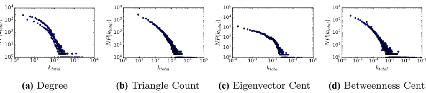
3.2 Power‑Law Feature Distribution

Many empirical graphs, especially those representing social, hyperlink and citation networks, have been shown to have approximately a power-law distribution of degree values [52]. This power-law distribution poses a challenge for machine learning models, as it means the features we are trying to predict are extremely unbalanced, with a heavy skew towards the lower range of features. Imbalanced class distribution creates difficulties for machine learning models, as there are fewer examples of the minority classes for the model to learn, which can often lead to poor predictive per-formance on these classes [14]. It has been shown that the distribution of other topological features can also follow a power-law distribution in many graphs [43]. To demonstrate this phenomenon, Fig. 1 shows the distribution of a range of topological feature values for the cit-HepTh dataset. The figure shows that indeed, all the topological feature values tested largely follow an approximately power-law distribu-tion. This fact has the potential to make predicting the value of a certain topological feature challenging, as the datasets will not be balanced and any model attempted to find the mapping f ∶ℝd

→𝛬 will be prone to over-fitting to the majority classes. Our approach for tackling this issue is out-lined in the following section.

3.3 Methodology

Unlike previous studies [44] we employ classification and visualisation, instead of regression, as ways to explore the embedding space. We chose these approaches as predicting topological features directly via the use of regression has proven challenging in prior work [44], owing largely to the imbalance problem explored in the previous section. With such an imbalanced dataset, using a classification-based approach is often advantageous [53] as techniques exist to over-sample minority examples. However, the features we are attempting to predict are continuous, so must go through some transformation stage before classification can be per-formed. For our transformation stage, we follow a procedure

5 _{Hops represent the length of the sequences of vertices that must}

similar to that introduced by Oord et al. [53]. We bin the real-valued features into a series of classes via the use of a histogram, where the bin in which a particular feature is placed becomes its class label. One can consider each of these newly created classes as representing a range of pos-sible values for a given feature. As an example, we could transform a vertex’s continuous PageRank score [8] into a series of discrete classes via the use of a histogram with a bin size of three, where each of the newly created classes represented a low, medium or high PageRank score.

Although this binning process helps with the feature imbalance, it still produces a skew in number of features assigned to each class. To further address this issue, we take the logarithm of each feature value before it is passed to the binning function. Essentially, this will mean that features within the same order of magnitude will be assigned the same class; for example, vertices with degrees in the range of 0–101 would be assigned into one class, whilst degree

val-ues between 102 and ₁₀3 would be assigned to another class.

This was performed as it dramatically improved the balance of the datasets, and as we are only attempting to discover if something approximating the topological features is present in the embedding space, we found that predicting the order of magnitude to be sufficient.

In order to allow for a good distribution of feature values in the datasets we are using, in our experiments we utilise a bin size of six for the histogram function, meaning that six discrete classes were created for each of the features. This value was chosen empirically from our datasets as it fully covered the numerical range of the topological features we measured. For example, we found that the centrality values in our datasets fall within a range of six orders of magnitude, which is what we used to set the number of bins. It should be noted that this value would need to be tuned depending upon the datasets and features being used.

In addition to the use of classification, we explore an addi-tional method to bring interpretability to graph embeddings, that being a visualisation technique entitled t-SNE [54]. This technique allows relatively high-dimensional data, such as graph embeddings, to be projected into a low-dimensional

space in such a way as to preserve the inter-spatial relation-ship between points that were present in the original space. Thus, we utilise t-SNE to project the embeddings down to two dimensions, so they can be easily visualised. This pro-cess is performed without the need for any classification to be trained upon the embeddings, removing the issues associated with classifying unbalanced datasets. Once the projection has been performed, we can colour each point in accordance with its feature value, be that one that has been transformed via the binning process, or even the raw value itself.

3.4 Embedding Approaches Compared

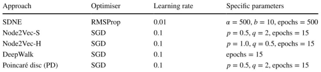
In this paper, we evaluate five state-of-the-art unsupervised graph embedding approaches as a way of exploring what semantic content is extracted from a graph to create the embed-dings. The approaches are as follows: DeepWalk, Poincaré disc, structural deep network embedding and Node2Vec,6

which are detailed in Table 1. These approaches were chosen as they represent a good cross section of the current compet-ing methodologies and all either exploit a different method of sampling the graph, use different geometries for the embed-ding space or use competing methods of comparing vertices. This selection of approaches will allow exploration of interest-ing research questions. Such questions include if any differ-ences between the approaches can be explained by what graph structures they learn and do methods which promote local

Table 1 _{Graph embedding approaches being compared}

Approach Year Type Published Complexity DeepWalk 2014 Stochastic KDD [4] O(|V|) Node2Vec 2016 Stochastic KDD [5] O(|V|) SDNE 2016 Auto-encoder KDD [37] O(|V||E|) Poincaré disc 2017 Hyperbolic MLG [32] O(|V|)

6 _{Please note that we explore two variations of Node2Vec, bringing}

the total number of approaches to five.

(a) Degree (b) Triangle Count (c) Eigenvector Cent (d) Betweenness Cent

Fig. 1 Distribution of topological feature values from the cit-HepTh dataset in log scale: a total vertex degree distribution, b distribution of com-plete triangles for each vertex, c eigenvector centrality distribution and d betweenness centrality score distribution

exploration around the target vertex only learn local structural information, degree for example. To explore this second ques-tion in more detail, we created two versions of Node2Vec: Node2Vec-Structural, which biases the random walks used to create training pairs for the model to explore vertices further away from the target vertex, and Node2Vec-Homophily, which biases the random walks to stay closer to the target vertex.

4 Experimental Set‑up and Classification

Algorithm Selection

In the following section we detail the set-up of the experi-ments and evaluate potential classification algorithms.

4.1 Metrics

4.1.1 Presented Results

All the reported results are the mean of five replicated exper-iment runs along with confidence intervals. For the run-time analysis, the presented results are the mean run-time for job completion, presented in minutes. For the classifica-tion results, all the accuracy scores presented are the mean accuracy after k-fold cross-validation—considered the gold standard for model testing [55]. For k-fold cross-validation, the original dataset is partitioned into k equally sized parti-tions. k−1 partitions are used to train the model, with the

remaining partition being used for testing. The process is repeated k times using a unique partition for each repetition and a mean taken to produce the final result.

4.1.2 Precision Metrics

For reporting the results of the vertex feature classification tasks, we report the macro-f1 and micro-f1 scores with vary-ing percentages of labelled data available at trainvary-ing time. This is a similar set-up to previous works [2, 5].

The micro-f1 score calculates the f1-score for the data-set globally by counting the total number of true positives (TP), false positives (FP) and false negatives (FN) across a labelled dataset |L|. Using the notation from [2], micro-f1 is defined as: where (6) microf1= 2⋅P⋅R P+R , Precision(P) = ∑�L� l=1TP(l) ∑�L� l=1TP(l) +FP(l) , Recall(R) = ∑�L� l=1TP(l) ∑�L� l=1TP(l) +FN(l) ,

and TP(l) denotes the number of true positives the model

predicts for a given label l, FP(l) denotes the number of false

positives, and FN(l) denotes the number of false negatives.

The macro-f1 score, when performing multi-label clas-sification, is defined as the average micro-f1 score over the whole set of labels L:

where microf1(l) is the micro-f1 score for the given label l.

4.2 Experimental Set‑up

4.2.1 Implementation Details

The approaches used for experimentation were re-imple-mented in TensorFlow [56], as the author-provided versions were not all available using the same framework. We also ensure the same TensorFlow-based optimisations were used across all the approaches wherever possible [57]. Neural Networks contain many hyper-parameters a user can control to improve the performance, both of the predictive accuracy and the run-time, of a given dataset. This process can be extremely time consuming and often requires users to per-form a grid search over a range of possible hyper-parameter values to find a combination which performs best [14]. For setting the required hyper-parameters for the approaches, we used the default hyper-parameters as proposed by the authors in their original papers, keeping them constant across all datasets. The key hyper-parameters used for each approach are detailed in Table 2. We have open-sourced our imple-mentations of these approaches and made them available online.7

4.2.2 Experimental Environment

Experimentation was performed on a compute system with 2 NVIDIA Tesla K40c’s, 2.3 GHz Intel Xeon E5-2650 v3, 64 GB RAM and the following software stack: Ubuntu Server 16.04 LTS, CUDA 9.0, CuDNN v7, TensorFlow 1.5, scikit-learn 0.19.0, Python 3.5 and NetworkX 2.0.

4.2.3 Experimental Datasets

The empirical datasets used for evaluation were taken from the Stanford Network Analysis Project (SNAP) data reposi-tory [58] and the Network Repository [59] and are detailed in Table 3. The domain label provided is taken from the (7) macrof1= 1 |L_| ∑ l∈L micro-f1(l),

listings of the graphs domain provided by SNAP [58] and Network Repository [59].

4.3 Classification Algorithm Selection

As highlighted throughout the paper, we are focusing our research on unsupervised graph embedding approaches. In order to be able to use the embeddings for further analy-sis, they must be classified using a supervised classification model. Traditionally in the embedding literature, a simple logistic regression is used in any classification task [4, 28], with seemingly little work exploring the use of more sophis-ticated models to perform the classification.

In this section we explore the effectiveness of five differ-ent models at performing the classification of the differdiffer-ent embedding approaches—logistic regression (LR), support vector machine (SVM) (linear kernel), SVM (RBF kernel), a single hidden layer neural network and finally a second more complex neural network with two hidden layers and a larger number of hidden units. All the classifiers utilised in this section were taken from the Scikit-Learn Python package [60]. Additionally, given that our datasets do not have a equal distribution among the classes, we also explore the effectiveness of weighting the loss function used by the model inversely proportional to the frequency of the class [61]. This use of a weighted loss function, although common in other areas of machine learning, has not been explored in regard to graph embeddings.

For the results in this section, we present the mean macro- and micro-f1 scores, introduced in Sect. 4.1.2, after fivefold cross-validation. To assess the performance of the classifiers against the imbalance present in the datasets, we also display

the percentage lift in mean test set accuracy over three rule-based prediction methods to act as baselines. These methods are uniform prediction (where the classification of each item in the test is chosen uniformly at random from the possible classes), stratified prediction (where the classification fol-lows the distribution of classes in the training set) and fre-quent class prediction (where the classification is determined by the most frequency class in the training set). A positive lift across all metrics strongly suggests that a mapping from the embedding space to the topological features is being learned, as the classification algorithm is overcoming the biased distributions of classes in the dataset.

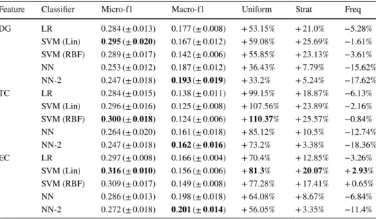
We performed this experiment for all combinations of datasets, embedding approaches and features, but due to the large quantity of results, we present only a subset here. Spe-cifically, we present the results for ego-Facebook dataset, using embeddings generated by DeepWalk and SDNE and classifying degree, triangle count and eigenvector central-ity. It should be noted that the patterns displayed here are representative of ones seen across all datasets.

Table 4 highlights the performance of the potential clas-sifiers, when using the DeepWalk embeddings taken from the ego-Facebook dataset. Results show that the choice of supervised classifier can have a large impact on the over-all classification score. It can also be seen that the tradi-tional choice of logistic regression does not produce the best results. Indeed, the neural network and SVM classifier often gave the best scores, but no single classifier is best overall, suggesting that one needs to be chosen carefully for a given task.

Table 5 highlights the results for the potential classifi-ers, when using the SDNE embeddings taken from the ego-Facebook dataset. Again, the variation in classification score across the set of tested classification metrics is quite sub-stantial, with the linear SVM and neural network approaches having perhaps a small margin of improvement over the others. It is interesting to note that the logistic regression frequently used in the literature never has the highest score in any metric. It can also be seen that, when compared to the DeepWalk results in Table 4, SDNE does less well at predicting all topological features which, although not the explicit purpose of this section, is interesting to note.

Using the results from this section, particularly the generally higher macro-f1 scores which indicate a better

Table 3 _{Empirical graph datasets}

Dataset |V| |E| Domain Source Fly-drosophila-medulla 1800 33,500 Biological [59] Cit-HepTh 27,770 352,807 Citation [58] Email-Eu-core 1005 25,571 Communication [58] Inf-openflights 2900 30,500 Infrastructure [59] Soc-sign-bitcoinotc 5881 35,592 Blockchain [58] Ego-Facebook 4039 88,234 Social [58]

Table 2 Key hyper-parameter

settings Approach Optimiser Learning rate Specific parameters

SDNE RMSProp 0.01 𝛼=500 , b=10 , epochs=500

Node2Vec-S SGD 0.1 p=0.5 , q=2 , epochs=15

Node2Vec-H SGD 0.1 p=1.0 , q=0.5 , epochs=15

DeepWalk SGD 0.1 epochs=₁₅

prediction across all classes, all the classification results in Sect. 5 are presented using a single hidden layer neural network.

5 Results

This section presents both the supervised and unsuper-vised results for predicting topological features from graph embeddings.

5.1 Topological Feature Prediction

In this section, we present the experimental evaluation of the classification of topological features using the embeddings generated from the five approaches (DeepWalk, Node2Vec-H, Node2Vec-S, SDNE and PD) on the datasets detailed in Table 3. We present both the macro-f1 and micro-f1 scores plotted against a varying amount of labelled data available during the training process, where a higher score equates to

Table 4 Degree (DG), triangle count (TC) and eigenvector centrality (EC) classification results for DeepWalk embeddings on the ego-Facebook dataset

Results for micro- and macro-f1 scores are the mean after fivefold cross-validation, with standard devia-tions. Lifts over uniform, stratified and frequency predictors are presented as percentages

Bold values indicate the best for that metric

Feature Classifier Micro-f1 Macro-f1 Uniform Strat Freq

DG LR 0.336(±0.015) 0.190(±0.012) +65.09% +33.85% +12.07% SVM (Lin) 𝟎.𝟑𝟑𝟗(±𝟎.𝟎𝟏𝟕) 0.164(±0.013) +𝟔𝟔.𝟓𝟕% +𝟑𝟓.𝟎𝟑% +𝟏𝟑.𝟎𝟕% SVM (RBF) 0.336(±0.021) 0.158(±0.013) +65.09% +33.84% +12.07% NN 0.329_(±0.013₎ 𝟎.𝟐𝟎𝟎_(±𝟎.𝟎𝟏𝟖_{) +}61.65_{% +}31.05_{% +}9.73_% NN-2 0.326(±0.016) 0.192(±0.019) +60.18% +29.85% +8.73% TC LR 0.340(±0.011) 0.154(±0.014) +109.34% +37.19% +12.38% SVM (Lin) 𝟎.𝟑𝟒𝟒(±𝟎.𝟎𝟏𝟓) 0.139(±0.006) +𝟏𝟏𝟏.𝟖% +𝟑𝟖.𝟖% +𝟏𝟑.𝟕% SVM (RBF) 0.335(±0.018) 0.130(±0.010) +106.26% +35.17% +10.73% NN 0.331(±0.019) 0.157(±0.013) +103.8% +33.56% +9.4% NN-2 0.326(±0.017) 𝟎.𝟏𝟔𝟑(±𝟎.𝟎𝟏𝟓) +100.72% +31.54% +7.75% EC LR 0.590_(±0.013₎ 0.474_(±0.010_{) +}195.66_{% +}144.16_{% +}92.18_% SVM (Lin) 0.591(±0.012) 0.480(±0.011) +196.16% +144.58% +92.51% SVM (RBF) 0.552(±0.012) 0.446(±0.011) +176.62% +128.44% +79.8% NN 0.629(±0.012) 0.512(±0.017) +215.2% +160.3% +104.89% NN-2 𝟎.𝟔𝟑𝟎(±𝟎.𝟎𝟏𝟗) 𝟎.𝟓𝟏𝟑(±𝟎.𝟎𝟐𝟏) +𝟐𝟏𝟓.𝟕% +𝟏𝟔𝟎.𝟕𝟐% +𝟏𝟎𝟓.𝟐𝟏%

Table 5 Degree (DG), triangle count (TC) and eigenvector centrality (EC) classification results for SDNE embeddings on the ego-Facebook dataset

Results for micro- and macro-f1 scores are the mean after fivefold cross-validation, with standard devia-tions. Lifts over uniform, stratified and frequency predictors are presented as percentages

Bold values indicate the best for that metric

Feature Classifier Micro-f1 Macro-f1 Uniform Strat Freq DG LR 0.284(±0.013) 0.177(±0.008) +53.15% +21.0% −5.28% SVM (Lin) 𝟎.𝟐𝟗𝟓(±𝟎.𝟎𝟐𝟎) 0.167(±0.012) +59.08% +25.69% −1.61% SVM (RBF) 0.289(±0.017) 0.142(±0.006) +55.85% +23.13% −3.61% NN 0.253(±0.012) 0.187(±0.012) +36.43% +7.79% −15.62% NN-2 0.247(±0.018) 𝟎.𝟏𝟗𝟑(±𝟎.𝟎𝟏𝟗) +33.2% +5.24% −17.62% TC LR 0.284(±0.015) 0.138(±0.011) +99.15% +18.87% −6.13% SVM (Lin) 0.296(±0.016) 0.125(±0.008) +107.56% +23.89% −2.16% SVM (RBF) 𝟎.𝟑𝟎𝟎(±𝟎.𝟎𝟏𝟖) 0.124(±0.006) +𝟏𝟏𝟎.𝟑𝟕% +25.57% −0.84% NN 0.264(±0.020) 0.161(±0.018) +85.12% +10.5% −12.74% NN-2 0.247(±0.018) 𝟎.𝟏𝟔𝟐(±𝟎.𝟎𝟏𝟔) +73.2% +3.38% −18.36% EC LR 0.297(±0.008) 0.166(±0.004) +70.4% +12.85% −3.26% SVM (Lin) 𝟎.𝟑𝟏𝟔(±𝟎.𝟎𝟏𝟎) 0.156(±0.006) +𝟖𝟏.𝟑% +𝟐𝟎.𝟎𝟕% +𝟐.𝟗𝟑% SVM (RBF) 0.309(±0.017) 0.149(±0.008) +77.28% +17.41% +0.65% NN 0.286(±0.013) 0.198(±0.018) +64.08% +8.67% −6.84% NN-2 0.272(±0.018) 𝟎.𝟐𝟎𝟏(±𝟎.𝟎𝟏𝟒) +56.05% +3.35% −11.4%

a better classification result—with a score of one meaning a perfect classification of every example in the data.

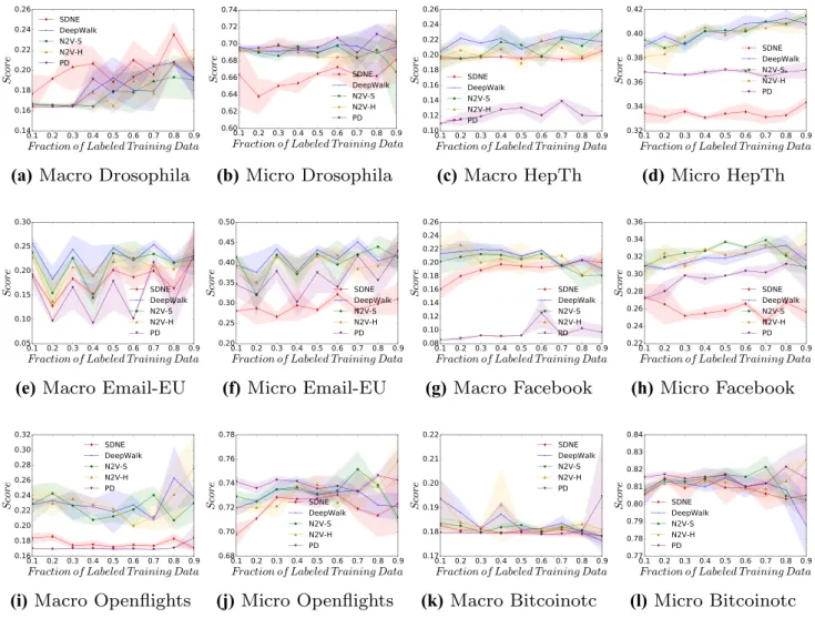
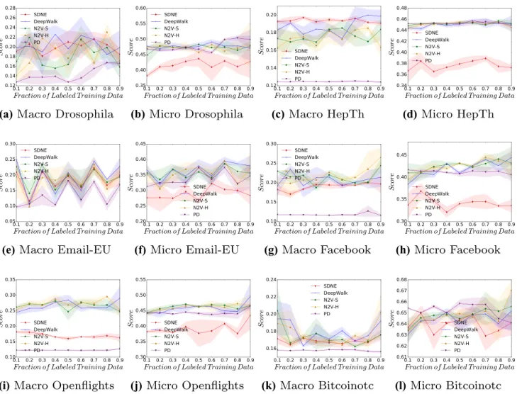
Figure 2 displays the classification of f1 scores for pre-dicting the simplest feature we are measuring: the degree of the vertices. Interestingly, we see a large spread of results across the datasets and between approaches, with no clear pattern emerging in this figure. On certain datasets, it is possible to see a high micro-f1 score, for example in the Bitcoinotc dataset, suggesting that an approximation of the degree value is present in the embedding. The figure also shows that SDNE and PD often have a lower score when compared to the stochastic approaches.

Figure 3 highlights the macro-f1 and micro-f1 scores for the classification of the degree centrality value. As the degree centrality of a given vertex is strongly influenced by its degree, it is perhaps unsurprising to observe largely similar patterns to those in Fig. 2, which again shows the dataset Bitcoinotc to be the dataset with the highest accu-racies. As seen in the previous figure, generally the three

stochastic approaches have a similar score for both macro-f1 and micro-f1.

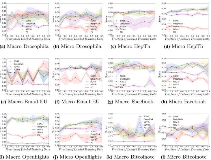
The results for the classification of triangle count for the vertices are presented in Fig. 4. This is a more complex fea-ture than the previous two, as it requires more information than is available from just the immediate neighbours of a given vertex. The figure shows again that, to some degree of accuracy, the feature is able to be reconstructed from the embedding space, with Bitcoinotc having the highest micro-f1 accuracy of all the datasets. SDNE and PD continue to have, on average, the lowest accuracies.

Classifying a vertex’s local clustering score across the datasets is explored in Fig. 5. The figure shows that this feature, although more complicated to compute than a ver-tex’s triangle count, appears to be easier for a classifier to reconstruct from the embedding space. With this more com-plicated feature, some interesting results regrading SDNE can be seen in the Email-EU and HepTh datasets, where the approach has the highest macro-f1 score—perhaps indicating

(a) Macro Drosophila (b) Micro Drosophila (c) Macro HepTh (d) Micro HepTh

(e) Macro Email-EU (f) Micro Email-EU (g) Macro Facebook (h) Micro Facebook

(i) Macro Openflights (j) Micro Openflights (k) Macro Bitcoinotc (l) Micro Bitcoinotc

Fig. 2 _{Micro- and macro-f1 scores, across a range of labelling fractions, for all approaches when predicting a vertex’s degree (DG) value across}

that the more complex model is better able to learn a good representation for this more complicated feature.

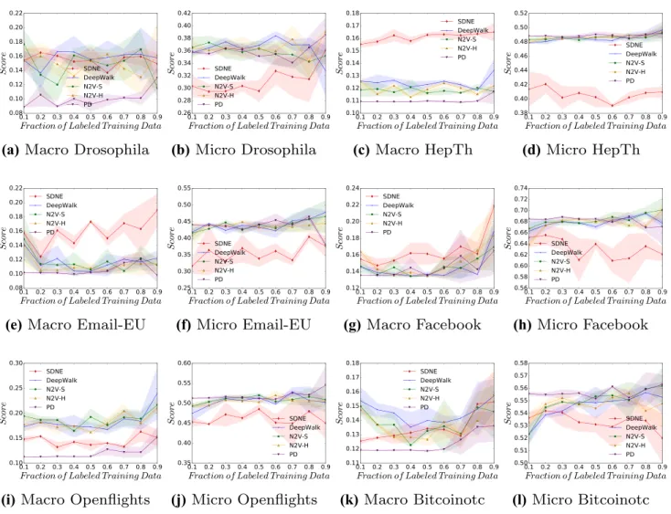
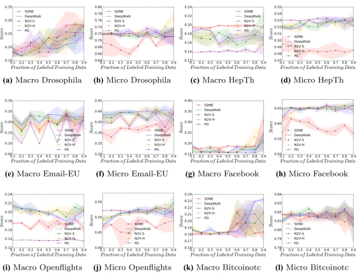
Figure 6 displays the result for the classification of a ver-tex’s eigenvector centrality. This figure is perhaps the most interesting one so far as it shows high classification accura-cies across many of the empirical datasets, even though this feature is of greater complexity than previous ones. This fig-ure further supports the results presented in Table 4, which shows eigenvector centrality having not only the highest accuracies, but also the highest lifts in accuracy over the rule-based predictors. Interestingly, SDNE does not demon-strate higher macro-f1 scores in this experiment.

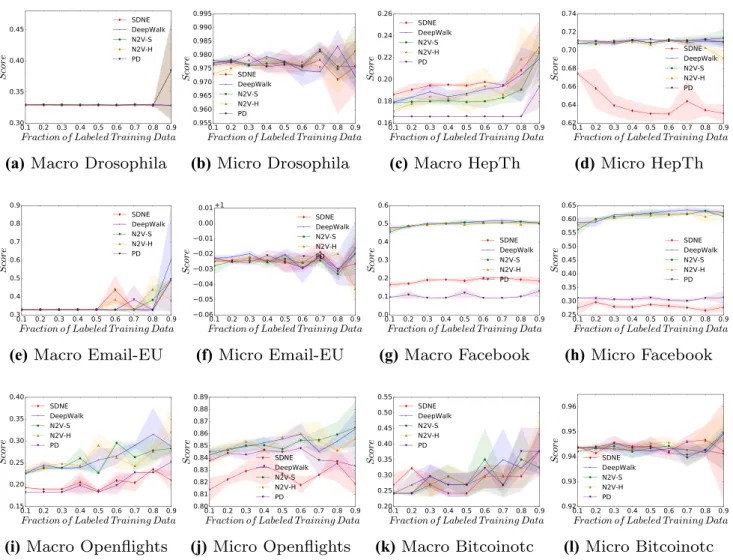
In Fig. 7, the approach’s ability to correctly classify the PageRank score of the vertices is considered. Here we see generally lower classification accuracies than the last figure, perhaps owing to the more complicated nature of the PageR-ank algorithm. However, high classification accuracies can still be seen, particularly on the Bitcoinotc and Drosophila datasets.

Finally, Fig. 8 highlights the ability of the graph embed-dings to predict betweenness centrality. Here, the figure shows that this feature is, on average, harder to predict from the embeddings than the previous two centrality measures as evidenced by the lower accuracy scores. Again, SDNE shows the highest macro-f1 scores on the Drosophila and HepTh datasets, indicating its embedding captures some-thing akin to this structural information better than the other approaches.

5.2 Confusion Matrices

One consideration that must be made is that the binning process, used to transform the features into targets for classi-fication, removes the inherent ordering present in continuous values. As an example, a vertex with a degree of 8 would still be classified incorrectly if the prediction was 10 or 100, but clearly one is more incorrect than the other. To address this, we present a selection of error matrices, to explore how

(a) Macro Drosophila (b) Micro Drosophila (c) Macro HepTh (d) Micro HepTh

(e) Macro Email-EU (f) Micro Email-EU (g) Macro Facebook (h) Micro Facebook

(i)Macro Openflights (j) Micro Openflights (k) Macro Bitcoinotc (l)Micro Bitcoinotc

Fig. 3 _{Micro- and macro-f1 scores, across a range of labelling fractions, for all approaches when predicting a vertex’s degree centrality (DG)}

‘wrong’ an incorrect prediction is. This is made possible as the labels used for classification have consecutive ordering, as a result of a histogram binning function, meaning that a prediction of 2 for a true label of 1 is more correct than a prediction of 5.

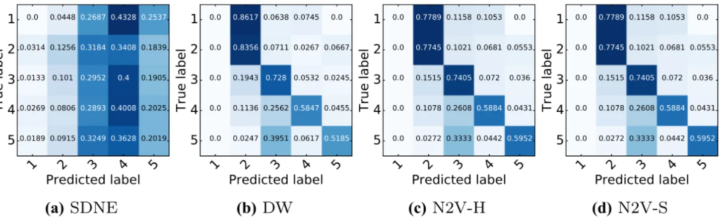
For brevity, Fig. 9 displays the error matrices for a selec-tion of the tested embedding approaches when classifying eigenvector centrality in the ego-Facebook dataset, although similar patterns were found across all datasets. With error matrices, the diagonal values represent correctly classified label; thus, a good prediction will produce an error matrix with a higher concentration of diagonal values. Figure 9

shows that, for the stochastic walk approaches DeepWalk and Node2Vec, the error matrices have a higher clustering of values around the diagonals. Interestingly, when the clas-sification is incorrect for these approaches, the incorrect pre-diction tends to be close to the true label. This phenomenon can clearly be seen in these approaches for labels 1 and 2, meaning that embeddings for vertices with these particularly

eigenvector centrality are similar. The figure also shows that, for this particular vertex feature, the embeddings produced via SDNE seemingly do not contain the same topological information. This is highlighted by the lack of structure on the diagonals of its error matrix.

5.3 Unsupervised Low‑Dimensional Projections

Figure 10 displays a selection of t-SNE plots taken from the ego-Facebook data, where the points are coloured according to the eigenvector centrality value after being passed through the binning process. The figure shows that the SDNE embed-dings seemingly have no clear structure in the low-dimen-sional space which correlates strongly with the eigenvec-tor centrality, as points in the same class are not clustered together. However, with the other embedding approaches, it is possible to see a clear clustering of points belonging to the same class. For example, in both the Node2Vec approaches, there is very clear clustering of classes one, four and five.

(a)

Macro Drosophila

(b)

Micro Drosophila

(c)

Macro HepTh

(d)

Micro HepTh

(e)

Macro Email-EU

(f)

Micro Email-EU

(g)

Macro Facebook

(h)

Micro Facebook

(i)

Macro Openflights

(j)

Micro Openflights

(k)

Macro Bitcoinotc

(l)

Micro Bitcoinotc

Fig. 4 _{Micro- and macro-f1 scores, across a range of labelling fractions, for all approaches when predicting a vertex’s triangle count (TR) value}

This result provides further evidence for our observation that, even when exploring the embeddings using an unsu-pervised method, it is possible to find correlations between known topological features and the embedding space.

5.4 Auto‑encoder Comparison

The results presented thus far have shown that it can be comparatively challenging to recover evidence of topologi-cal features from the auto-encoder-based SDNE approach. To investigate this further, we compare SDNE with another auto-encoder-based approach entitled DNGR. Unlike the other approaches tested thus far, DNGR mandates the use of weighted graphs. However, from the empirical datasets we are using for this study, only the soc-sign-bitcoinotc dataset contains weighted edges, which represent the level of trust which users place in each other.

To investigate if DNGR captures more recognisable topo-logical structure in its embedding space, we will again use

(a) Macro Drosophila (b) Micro Drosophila (c) Macro HepTh (d) Micro HepTh

(e) Macro Email-EU (f) Micro Email-EU (g) Macro Facebook (h) Micro Facebook

(i)Macro Openflights (j) Micro Openflights (k) Macro Bitcoinotc (l)Micro Bitcoinotc

Fig. 5 _{Micro-f1 and macro-f1 scores, across a range of labelling fractions, for all approaches when predicting a vertex’s local clustering}

coef-ficient (CLU) value across all datasets

t-SNE. However, the soc-sign-bitcoinotc dataset has the low-est edge density of any of the graphs we are tlow-esting, resulting in a very unbalanced dataset. (For example, the majority of the vertices have a very low degree value.) To allow for greater insight, here we chose not to use the binning process to label each vertex embedding. Instead, we normalise the raw topological feature values to be between zero and one; we then use this value to directly colour the points on the t-SNE plots. Here we would expect to see points of a simi-lar colour, and thus feature value, to be clustered together if vertices with similar topological features are close in the underlying embedding space. Due to soc-sign-bitcoinotc having a larger number of vertices than the dataset used for the previous t-SNE visualisation, we plot only a randomly selected half of the vertices to allow for clearer figures.

Figure 11 displays the t-SNE plots of the vertex embed-dings for both SDNE and DNGR across four different top-ological features. The figure shows that despite it being more challenging to recover topological features from

SDNE in other experiments, there is still structure pre-sent in the embedding space correlating to several top-ological features. One can see SDNE embeddings with similar feature values being clustered together in these plots; for example, there are clear clusters of vertices with a high and low degree, PageRank and betweenness cen-trality value visible, whereas it is much harder to inter-pret any structure in the embedding space produced via DNGR. This could well be due to the fact that DNGR does not take as input the raw adjacency matrix; instead, it is reconstructing the PPMI matrix, capturing vertex co-occurrence. Due to this transformed input, it is perhaps not surprising that normal topological features are present in the resulting representations.

5.5 Discussion

This section has provided extensive experimentation evalu-ation to explore the questions raised in Sect. 3. Specifically,

we investigated if a broad range of topological features can be predicted from the embedding created from a range of unsupervised graph embedding techniques. Across all the features and datasets tested, it can be seen that many topological features can be approximated by the different embedding approaches, with varying degrees of accuracy. The results which show the increase in accuracy over the rule-based predictions (Sect. 4.3) give strong indication that the approaches are able to overcome the inherent unbalanced nature of graph datasets and a mapping from the embedding space to features is present. It is also interesting to observe that numerous features can be approximated from the graph embeddings, suggesting that several structural properties are being captured to create the best representation for a vertex automatically. Of all the topological features measured in the experimentation section, the one which consistently gave the best results was eigenvector centrality. Particularly for the stochastic approaches, eigenvector centrality was pre-dicted with a high degree of accuracy, suggesting that the

(a) Macro Drosophila (b) Micro Drosophila (c) Macro HepTh (d) Micro HepTh

(e) Macro Email-EU (f) Micro Email-EU (g) Macro Facebook (h) Micro Facebook

(i) Macro Openflights (j) Micro Openflights (k) Macro Bitcoinotc (l) Micro Bitcoinotc

Fig. 6 _{Micro-f1 and macro-f1 scores, across a range of labelling fractions, for all approaches when predicting a vertex’s eigenvector centrality}

topological structure represented by this feature is captured extremely well in the embedding space and indicates this is a useful feature for minimising the objective functions of the approaches. This is further reinforced by the unsupervised projections (Fig. 10), which shows clear and distinct cluster-ing between classes, even without the use of a classification algorithm.

Another interesting observation from this study is that no one approach strongly outperforms the others when classifying a particular feature—seemingly all the approaches are approxi-mating similar topological structures. The figures show that the stochastic approaches (DeepWalk and Node2Vec) are the most consistent across all features and datasets, often having the highest macro-f1 and micro-f1 scores. SDNE demonstrates a more inconsistent performance profile for feature classifica-tion; this is in contrast to other studies which have found it to have the best performance in vertex labelling problems [2]. The performance of SDNE demonstrated in this work could be explained by it being the only deep model tested, meaning

that it contains many more parameters. This increase in com-plexity means that SDNE could be very sensitive to the correct selection of hyper-parameters or possibly that more complex topological features are being approximated by the embed-dings—or even that entirely novel features are being learned. Finally, it is interesting to note the performance of hyperbolic (PD) approach, which has far fewer latent dimensions in which to capture topological information due to its limitation in mod-elling the space as a 2D disc. Empirically, PD shows largely similar performance to the other approaches on most data-sets, providing strong evidence that the hyperbolic space is an appropriate space in which to represent graphs.

6 Conclusion

Graph embeddings are increasingly becoming a key tool to solve numerous tasks within the field of graph mining. They have demonstrated state-of-the-art results by reporting to

(a) Macro Drosophila (b) Micro Drosophila (c) Macro HepTh (d) Micro HepTh

(e) Macro Email-EU (f) Micro Email-EU (g) Macro Facebook (h) Micro Facebook

(i) Macro Openflights (j) Micro Openflights (k) Macro Bitcoinotc (l) Micro Bitcoinotc

Fig. 7 _{Micro-f1 and macro-f1 scores, across a range of labelling fractions, for all approaches when predicting a vertex’s PageRank (PR) value}