Digital twins: Understanding the added value of integrated models for through-life engineering services

(1)

City, University of London Institutional Repository

Citation

:

Vrabič, R., Erkoyuncu, J. A., Butala, P. and Roy, R. ORCID:

0000-0001-5491-7437 (2018). Digital twins: Understanding the added value of integrated models for

through-life engineering services. Procedia Manufacturing, 16, pp. 139-146. doi:

10.1016/j.promfg.2018.10.167

This is the published version of the paper.

This version of the publication may differ from the final published

version.

Permanent repository link:

https://openaccess.city.ac.uk/id/eprint/24018/

Link to published version

:

http://dx.doi.org/10.1016/j.promfg.2018.10.167

Copyright and reuse:

City Research Online aims to make research

outputs of City, University of London available to a wider audience.

Copyright and Moral Rights remain with the author(s) and/or copyright

holders. URLs from City Research Online may be freely distributed and

linked to.

City Research Online:

http://openaccess.city.ac.uk/

[email protected]

(2)

ScienceDirect

Available online at _{Available online at}www.sciencedirect.com_{www.sciencedirect.com}

ScienceDirect

Procedia Manufacturing 00 (2017) 000–000

www.elsevier.com/locate/procedia

* Paulo Afonso. Tel.: +351 253 510 761; fax: +351 253 604 741 E-mail address: [email protected]

Peer-review under responsibility of the scientific committee of the Manufacturing Engineering Society International Conference 2017.

Manufacturing Engineering Society International Conference 2017, MESIC 2017, 28-30 June

2017, Vigo (Pontevedra), Spain

Costing models for capacity optimization in Industry 4.0: Trade-off

between used capacity and operational efficiency

A. Santana

a

_{, P. Afonso}

a,*

_{, A. Zanin}

b

_{, R. Wernke}

b a_{University of Minho, 4800-058 Guimarães, Portugal}

b_{Unochapecó, 89809-000 Chapecó, SC, Brazil}

Abstract

Under the concept of "Industry 4.0", production processes will be pushed to be increasingly interconnected, information based on a real time basis and, necessarily, much more efficient. In this context, capacity optimization goes beyond the traditional aim of capacity maximization, contributing also for organization’s profitability and value. Indeed, lean management and continuous improvement approaches suggest capacity optimization instead of maximization. The study of capacity optimization and costing models is an important research topic that deserves contributions from both the practical and theoretical perspectives. This paper presents and discusses a mathematical model for capacity management based on different costing models (ABC and TDABC). A generic model has been developed and it was used to analyze idle capacity and to design strategies towards the maximization of organization’s value. The trade-off capacity maximization vs operational efficiency is highlighted and it is shown that capacity optimization might hide operational inefficiency.

Peer-review under responsibility of the scientific committee of the Manufacturing Engineering Society International Conference 2017.

Keywords: Cost Models; ABC; TDABC; Capacity Management; Idle Capacity; Operational Efficiency 1. Introduction

The cost of idle capacity is a fundamental information for companies and their management of extreme importance in modern production systems. In general, it is defined as unused capacity or production potential and can be measured in several ways: tons of production, available hours of manufacturing, etc. The management of the idle capacity

This is an open access article under the CC BY-NC-ND license (https://creativecommons.org/licenses/by-nc-nd/4.0/)

Peer-review under responsibility of the scientific committee of the 7th International Conference on Through-life Engineering Services. 10.1016/j.promfg.2018.10.167

10.1016/j.promfg.2018.10.167 2351-9789

Peer-review under responsibility of the scientific committee of the 7th International Conference on Through-life Engineering Services. Available online at www.sciencedirect.com

7th International Conference on Through-life Engineering Services

Digital twins: Understanding the added value of integrated models

for through-life engineering services

Rok Vrabiˇc

a,∗

_{, John Ahmet Erkoyuncu}

b

_{, Peter Butala}

a

_{, Rajkumar Roy}

b

a_{University of Ljubljana, Department of Manufacturing Systems and Control, Slovenia}

b_{Cranfield University, Through-life Engineering Services Centre, United Kingdom}

Abstract

Digital twins are digital representations of physical products or systems that consist of multiple models from various domains describing them on multiple scales. By means of communication, digital twins change and evolve together with their physical counterparts throughout their lifecycle. Domain-specific partial models that make up the digital twin, such as the CAD model or the degradation model, are usually well known and provide accurate descriptions of certain parts of the physical asset. However, in complex systems, the value of integrating the partial models increases because it facilitates the study of their complex behaviours which only emerge from the interactions between various parts of the system. The paper proposes that the partial models of the digital twin share a common model space that integrates them through a definition of their interrelations and acts as a bridge between the digital twin and the physical asset. The approach is illustrated in a case of a mechatronic product – a differential drive mobile robot developed as a testbed for digital twin research. It is demonstrated how the integrated models add value to different stages of the lifecycle, allowing for evaluation of performance in the design stage and real-time reflection with the physical asset during its operation.

c

2018 The Authors. Published by Elsevier B.V.

Peer-review under responsibility of the scientific committee of the 7th International Conference on Through-life Engineering Services.

Keywords: digital twin ; modelling ; multi-domain model

1. Introduction

First coined in a product lifecycle management context in 2003 [1], digital twin is a concept that was envisioned well before the technology necessary for its implementation caught up. Initially, the digital twin was conceptualised as avirtual product- a rich representation of a product that is virtually indistinguishable from its physical counterpart. The initial concept included a data connection tying the virtual and the real product together throughout the lifecycle. Since the concept was conceived, tremendous advances have been achieved in the field of digital representation as

∗_{Corresponding author. Tel.:}₊_{386-1-4771-753.}

E-mail address:[email protected]

2351-9789 c2018 The Authors. Published by Elsevier B.V.

Available online at www.sciencedirect.com

7th International Conference on Through-life Engineering Services

Digital twins: Understanding the added value of integrated models

for through-life engineering services

Rok Vrabiˇc

a,∗

_{, John Ahmet Erkoyuncu}

b

_{, Peter Butala}

a

_{, Rajkumar Roy}

b

a_{University of Ljubljana, Department of Manufacturing Systems and Control, Slovenia}

b_{Cranfield University, Through-life Engineering Services Centre, United Kingdom}

Abstract

Digital twins are digital representations of physical products or systems that consist of multiple models from various domains describing them on multiple scales. By means of communication, digital twins change and evolve together with their physical counterparts throughout their lifecycle. Domain-specific partial models that make up the digital twin, such as the CAD model or the degradation model, are usually well known and provide accurate descriptions of certain parts of the physical asset. However, in complex systems, the value of integrating the partial models increases because it facilitates the study of their complex behaviours which only emerge from the interactions between various parts of the system. The paper proposes that the partial models of the digital twin share a common model space that integrates them through a definition of their interrelations and acts as a bridge between the digital twin and the physical asset. The approach is illustrated in a case of a mechatronic product – a differential drive mobile robot developed as a testbed for digital twin research. It is demonstrated how the integrated models add value to different stages of the lifecycle, allowing for evaluation of performance in the design stage and real-time reflection with the physical asset during its operation.

c

2018 The Authors. Published by Elsevier B.V.

Keywords: digital twin ; modelling ; multi-domain model

1. Introduction

First coined in a product lifecycle management context in 2003 [1], digital twin is a concept that was envisioned well before the technology necessary for its implementation caught up. Initially, the digital twin was conceptualised as avirtual product- a rich representation of a product that is virtually indistinguishable from its physical counterpart. The initial concept included a data connection tying the virtual and the real product together throughout the lifecycle. Since the concept was conceived, tremendous advances have been achieved in the field of digital representation as

∗_{Corresponding author. Tel.:}₊_{386-1-4771-753.}

E-mail address:[email protected]

2351-9789 c2018 The Authors. Published by Elsevier B.V.

(3)

140 Rok Vrabič et al. / Procedia Manufacturing 16 (2018) 139–146

2 R. Vrabiˇc, J.A. Erkoyuncu, P. Butala, R. Roy/Procedia Manufacturing 00 (2017) 000–000

well as in data collection and management technologies, and today the concept is receiving a lot of attention from the industry [2].

A recent pan-industry survey [3] found that much of the digital-twin-related technology is already available on the market, but that its integration still presents a challenge. In addition, the in-service phase has been highlighted by the industry as an area of significant potential benefit for the digital twin. A new definition that emphasises the through-life engineering aspects was proposed: “A digital twin is a digital representation of a physical item or assembly using integrated simulations and service data. The digital representation holds information from multiple sources across the product lifecycle. This information is continuously updated and is visualised in a variety of ways to predict current and future conditions, in both design and operational environments, to enhance decision making” [3].

Digital twins are nowadays considered as more than just collections of digital artefacts, but rather, as collections of linked digital artefacts. This distinction is a key one, and integrating and linking the models and the data still presents a research challenge. While partial models are able to address specific parts of the product, new behaviours can emerge when the models are intertwined. It is argued that the value of the digital twin primarily lies in the elimination of information inefficiencies which result in a waste of resources [4]. The assumption here is that, even though the information is never free to acquire or use, the cost of the information will be less than the cost of the wasted resources. But additional value can be derived from the integration of the models because this allows for a consideration of scenarios which exceed the descriptive capabilities of any single model.

The paper presents a concept of model integration within the digital twin, using a mobile robot as a test bed, and discusses the implications of the integration for added value in the context of through-life engineering services.

2. Integration of models within the digital twin

An often cited definition of the digital twin is that a digital twin is an ultra-high fidelity simulation, that when coupled with the specific vehicle health monitoring data, maintenance history and historical fleet data, can help to improve safety and reliability [5]. However other authors argue that the digital twin does not need to be an ultra-high fidelity simulation, but rather a reasonable estimation of the product operation [6]. They report that a digital twin of a complete airframe of an aircraft has 1012_{degrees of freedom and that if microstructure is considered, those models} have 107_{degrees of freedom at each location. This makes it impossible to simulate the behaviour of the system in real} time even with the current strongest supercomputers. Instead of focusing on the computational aspect, i.e. going into depth, not much is found in the literature about model complexity and combining the simulation and other models in a meaningful way, i.e. going into breadth [4].

This can be achieved by creating a common model space that allows the models to exchange the data, defines the relations between the models and acts as a bridge between the digital twin and the physical asset. Two kinds of relations between the models are defined. Aninput/outputrelation exists when a model needs the output of another

model as its input. For example, a CAM model takes the output of a part’s CAD model as its input and is then able to produce the NC code for part machining. Another kind of relation is aninfluencesrelation which specifies that a change in one of the model influences another model. For example, a tool wear model does not influence the CAD model but can be used to improve the CAM one. The common model space, therefore, defines how the models are connected as well as how and when they are updated.

The integrated model defined through the common model space also provides the capability to explore what-if scenarios. This is realised by alearning model. In addition to providing the simulation capability, the integrated model can use the learning model to support real-time reflection, interaction along the lifecycle, and self-evolution [7]. The learning model should, therefore, definehowto run the simulation, i.e. with what parameters. Consider, for example, how to ensure that the digital twin continues to represent the ever-changing physical asset. If a change is detected in the physical asset or its environment, the learning model should define simulation scenarios to explore which and how the model parameters have to be changed to mirror the observed behaviour. In other words, the learning model allows for real-time reflection through a simulation-based search through the parameter space.

The rest of the paper illustrates this idea and shows how it can be employed in various stages of a product lifecycle. A differential drive mobile robot with line following capability is considered. While it is a complex mechatronic product, its parts are simple enough to be analytically modelled. This, along with its ability to communicate in real time, makes the mobile robot a suitable test bed for digital twin research.

(4)

Rok Vrabič et al. / Procedia Manufacturing 16 (2018) 139–146 141

R. Vrabiˇc, J.A. Erkoyuncu, P. Butala, R. Roy/Procedia Manufacturing 00 (2017) 000–000 3

3. Digital twin of a mobile robot

The robot is based on an 8-bit microcontroller and is actuated by two geared DC motors. The robot’s sensors include an array of eight reflectance sensors facing downwards for line following, six reflectance sensors facing sideways for obstacle detection, a 9-axis inertial measurement unit (IMU), and encoders for detecting motor velocities. A Bluetooth module is used for real-time communication.

In this investigation, a line following task is considered. Although the principle of line following is simple, optimi-sation of the robot’s speed presents a challenge because of the many factors in play ranging from the robot’s geometry and dynamics, its hardware design, the control algorithms used, to responding to changes in the environment condi-tions while the task is performed.

3.1. Digital twin architecture

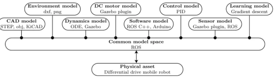
The architecture of the digital twin is based around loosely-coupled models that describe various aspects of the robot and its environment. Each of the models can be independently tested and calibrated to reflect the corresponding physical asset as closely as possible. To build the digital twin of the robot, Robot Operating System (ROS) is chosen as the basis for the common model space [8]. Fig.1shows the models along with the tools and formats that are used for their implementation. The rest of the section then details the models and shows how they can be integrated in the common model space.

Dynamics model ODE, Gazebo DC motor model Gazebo plugin Software model ROS C++, Arduino Control model PID Sensor model

Gazebo plugin, ROS

Learning model

Gradient descent

Common model space

ROS

CAD model

STEP, obj, KiCAD

Environment model

dxf, png

Physical asset

Dif erential drive mobile robotf

Fig. 1: Partial models of the digital twin.

The models include the CAD model, exported from the electronics design automation (EDA) software, in which the robot was designed. The environment model includes assets such as the track that are needed for line follower simulation. The motion model is implemented in Gazebo simulator and uses ODE physics engine. DC motors are simulated using a custom-made Gazebo plugin. A software model is developed that allows that the same code to be uploaded to the digital twin and the physical robot and makes sure that the code execution speeds are comparable. Line sensors are simulated using Gazebo’s camera plugin, while encoders are simulated by measuring the joint positions and velocities from the physics engine. A control model is developed for line following, along with a learning model which is able to optimise the control parameters and synchronise the digital twin with the physical asset. In order to understand the relations between the models shown in Fig.1and to be able to integrate them, a deeper understanding of their inputs, outputs, and parameters is necessary.

3.2. CAD model

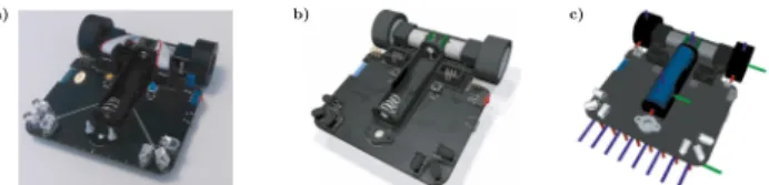
The CAD model is created in EDA software. All component models are imported or created in .STEP format. This allows for the final model to be exported to any other CAD software for further processing and analysis. Fig.

2shows the physical robot along with its CAD models in EDA software and in ROS, converted to Universal Robot Description Format (URDF) and visualised in ROS’s visualisation component RViZ. The CAD model defines the robot’s dimensions (L,R,S), and can be used to estimate masses and inertias of the robot platform and the wheels (mc,mw,Ic,Iw), and the location of the centre of gravity (d).

3.3. Model of motion

The model of motion describes robot’s kinematics and dynamics and is a core part of the robot’s digital twin. It is important for this model to be as accurate as possible in order to get the realistic behaviour of the robot in a

(5)

a) b) c)

Fig. 2: a) Real robot. b) CAD model in EDA software. c) CAD model in RViZ, showing robot’s frames.

simulation. The kinematic model describes the relationship between the velocities of the wheels and the translational and rotational velocities of the robot as well as the relation between the robot frame and the inertial frame. The coordinate systems are shown in Fig.3.

YI XI Xr Yr xa ya 2R 2L φ d (xc,yc) 0 L R Θ Θ S Legend Wheel Caster Line sensor Centre of gravity

Fig. 3: Differential drive mobile robot.

The position of the robot’s centre of rotation is denoted as (xa,ya), and it’s centre of gravity (COG) as (xc,yc). The

robot frame (Xr,Yr) moves with the robot and is rotated byφwith respect to the inertial frame (XI,YI). The linear

velocity of a differential drive mobile robot in the robot frame can be expressed as the average of the linear velocities of its wheels (Eq.1). The angular velocity of the robot depends on the difference of the linear speeds and the distance between the wheelsL(Eq.2). The robot kinematics in the inertial frame can be expressed with the translationalvand angularωvelocities as shown in Eq.3. The dynamic model is derived by using Lagrangian mechanics [9]. It is shown in [10] that the equations of motion can be expressed in terms ofvandωas shown in Eqs.4and5.

v= vR+vL 2 = R( ˙θR+θ˙L) 2 (1) ω= vR−vL 2L = R( ˙θR−θ˙L) 2L (2)    ˙ xa ˙ ya ˙ φ   =    cos(φ) 0 sin(φ) 0 0 1    v ω (3) (m+2Iw R2 )˙v−mcdω2= 1 R(τR+τL) (4) (I+2∗L 2 R2 Iw) ˙ω+mcdωv= L R(τr−τL) (5)

Wherem=mc+2mwis the total mass of the robot andI=Ic+mcd2+2mwL2+2Imis the total equivalent inertia.

Thus, the model of motion can be thought of as having the two motor torques (τr, τl) as the inputs, the translational

and rotational speeds (v, ω) as the outputs, subject to the parameters describing the mass, inertia, and the geometry of the robot (mc,mw,Ic,Iw,d,L,R). Besides, motion models are often executed by physics engines that enable a relaxation

of the kinematic constraints, e.g. by providing a simulation of friction, characterised by the friction coefficientmu. 3.4. DC motor model

The torques for the model of motion are produced by DC motors with permanent magnets. For an ideal DC motor, the motor torque is proportional to the armature currentiby a constant factor of K. The back emfUEMF, i.e. the

voltage that the motor is generating while its rotor is spinning in the magnetic field of the stator, is proportional to the angular velocity ˙θby the same factor (in SI units)K. The electric and the mechanical equations of an ideal DC motor is shown in Eqs.6and7respectively [11].

(6)

U=LMdi

dt+RMi+UEMF=LM di

dt +RMi+Kθ˙ (6)

Iwθ¨+bMθ˙=τ=Ki (7)

WhereUis the input voltage,LMandRMare inductance and resistance of the rotor windings, andbMis the viscous

friction. The DC motor model therefore has the voltageUas the input, the rotational velocity ˙θas the output, and the

following electrical and mechanical parameters (RM,LM,Iw,bM,K).

3.5. Sensor model

The line sensor is able to measure the position of the line below the robot by using an array of reflectance sensors made up from an infrared light source (LED) and a phototransistor. Since each sensor is only able to measure the changes in the amount of reflected light, the sensors need to be calibrated in the beginning. This is achieved by rotating the robot around its centre of rotation so that each sensor crosses the line multiple times. Minimum si,min

and maximumsi,maxsensor values are stored for each sensori. The raw sensor value si,rawis then scaled between 0

and 1000 to obtain the calibrated sensor valuesias shown in Eq.8. To estimate the position of the line, a weighted

average is calculated as shown in Eq.9. The angle of the line with respect to the robot’s centre of rotationlineangleis

considered to be the error signalefor the control model.

si=(si,raw_s −si,min)·1000

i,max−si,min (8)

lineangle=e=atan2 ((

N i=0si·i·1000 N i=0si − 3500)/100000,S) (9) 3.6. Control model

For the line following task, translational and rotational velocities are controlled. The chosen control policies are shown in Eqs. 10 and11, respectively. The translational velocity controller calculates the desired velocity as the absolute erroremultiplied by a control parameter KB and subtracted from a maximum velocity constantvmax. The

rotational velocity is controlled by a standard PID controller. The control loop is executed every∆t. The control model takes the erroreas the input signal, and generates translationalvand rotationalωvelocity signals to be executed by the robot’s microcontroller. The control is subject to five parameters: (vmax,KB,KP,KI,KD).

v=vmax−KB· |e| (10) ω=KP·e+KI· t 0 edt+KD· de dt (11) 3.7. Learning model

The role of the learning model is to enable simulation of what-if scenarios, which can then be used for different tasks such as optimisation of control parameters or synchronisation of the digital twin models with the physical asset. For the line following task, a gradient descent algorithm (Eq.12) with parameters as shown in Eq.13is chosen for the learning model.

xn+1=xn−γn∇F(xn) (12)

x=(vmax,KB,KP,KI,KD) (13)

The reason for choosing gradient descent as opposed to other machine learning techniques, such as genetic algo-rithms or neural networks, is that the problem space is mostly monotonic. For example, increasing the translational speed will almost always improve the performance of the line following task (measured by e.g. the lap time), up until the point that the task itself becomes unachievable, i.e. up to the point when the robot goes offtrack. Similarly, the lap time will almost certainly decrease if the tyre friction coefficient is reduced. Optimised values of parameters can, therefore, be found quickly with gradient descent, i.e. in a lower amount of completed laps and consequently in a lower amount of time.

(7)

The learning model implementation is as follows. The robot completes the first lap with initial parameters. The parameters are varied one by one in the following laps to estimate the gradient. The robot then completes a lap with the varied parameters and estimates parameters for a new round of gradient measurements (Eq.12). The procedure repeats for a fixed number of laps or until the parameters converge to their final values.

3.8. Model integration

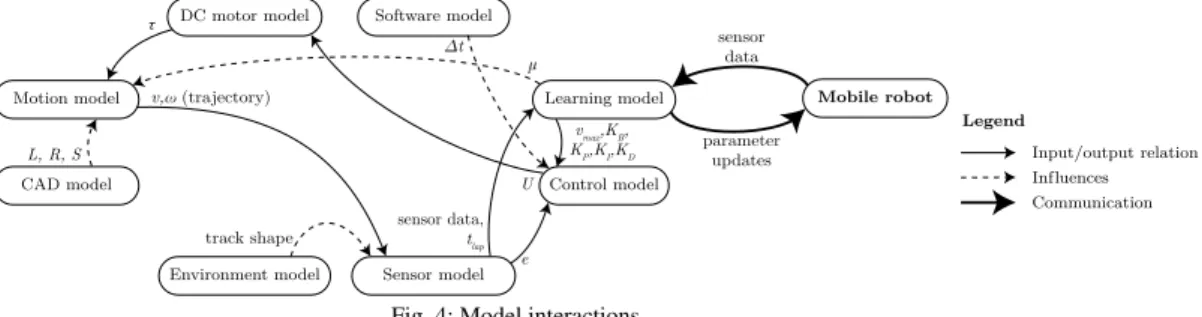
The integration of the above models within the common model space is essential if the digital twin is to accurately represent the changing behaviour of its physical counterpart. Fig.4shows how the models are related in the case of a line following task.

Motion model

DC motor model Software model

Control model Sensor model Learning model CAD model Environment model Legend Input/output relation Inf uencesl τ L, R, S sensor data, tlap v,ω (trajectory) e vmax,KB, KP,KI,KD U Δt track shape Mobile robot μ Communication sensor data parameter updates

Fig. 4: Model interactions.

The learning model takes care of synchronisation of the digital twin with the real robot through real-time commu-nication. The two inputs to the learning model are the sensor data from the sensor model and the sensor data from the robot. These are compared, and if there is a discrepancy, gradient descent is used to re-synchronise them through an exploration of what-if scenarios. Control parameters as well as physics parameters of the motion model, such as the coefficient of frictionµ, can be explored. The motion model converts the motor torquesτ, defined by the control

model and generated by the DC motor model, into translationalvand rotationalωvelocities, which can be integrated

by the physics engine to obtain the position of the robot in time, i.e. its trajectory. The sensor model then uses the current position of the robot and the track shape to generate simulated sensor data, closing the control loop.

The partial models are thus linked together into an integrated model that can be used to explore scenarios that no partial model can. The added value of this is that changes in any of the models or changes in the physical asset can be considered holistically, be it from the viewpoint of design or the viewpoint of real-time reflection. The cases that follow illustrate these examples.

4. Case studies

To illustrate the potential uses of the approach, two case studies are presented. The first one explores how the integrated models can be used to assess performance in the design stage using the learning model for control parameter optimisation. The second case study shows how changing conditions can be captured during operation and then reflected in the digital twin using the learning model.

4.1. Exploring the effect of design parameters on performance

It is difficult to assess the performance of complex products and systems in the design stage because of the intercon-nectedness of their parts and models. Typically, designs are modified using existing product knowledge. For example, an aircraft engine manufacturer almost never designs the product from scratch, but rather modifies the design parame-ters of an existing one incrementally, based on specific tests designed to improve part performance. Digital twins can assist in this process, but only if they are able to accurately represent the physical asset. Simulating the behaviour of the digital twin can then be used to explore what-if design scenarios. This case explores how the geometrical parame-ters of the design of the mobile robot influence its performance. As the geometry changes, so must the parameparame-ters of the control model, because, for example, a wider robot might need a stronger response to the error. The performance of modified designs can only be measured through concurrent optimisation of the control parameters. To do this, the

(8)

learning model (Eq.12) is employed. The robot performing the line following task is simulated. Each lap, the control parameters are optimised using gradient descent until they converge to their final values. Four scenarios, each with a different set of design parameters, are simulated. The results are shown in Fig.5.

0 20 40 60 80 100 120 140 13 500 14 000 14 500 15 000 15 500 16 000 16 500 lap[/] tlap [ms] a) b) 12 500 13 000 13 500 14 000 L=77 mm S=80.5 mmS=80.5 L=117 mmmmS=120.5 L=77 mmmmS=120.5 L=117 mmmm tlap [ms] c) 13916 13394 13093 12747

Fig. 5: a) The digital twin in the simulated environment. b) A typical gradient descent run. c) A distribution chart showing the effect of design parameters on performance.

In Fig.5a) the digital twin is shown in a simulated environment. A typical run of the simulation is shown in5b). The control parameters are changed using gradient descent and, in time, converge to their local optimums. Lap times from lap 100 forward, i.e. when the parameters converge and the lap times stabilize, are taken as the performance metric. Fig. 5c) shows how the final lap time depends on the modified geometrical design parameters. The results show that the initial design would benefit from increasing the distance between the wheelsLas well as from increasing the distance between the line sensors and the centre of rotationS. This is because the first change increases the overall torque for rotation which is the limiting factor (not the velocity of the rotation), and the second change increases the time the robot has to react to changes in track curvature, as placing the sensors further upfront can be thought of as looking further forward into the future from the perspective of the control model. In this case, the integrated model is used to link the design parameters, through simulation and learning, to the performance of the robot. An accurate simulation is not enough; software, control, and optimisation models also need to be linked and considered together in order to accurately asses the effect of design parameters on performance.

4.2. Digital twin alignment during operation

An important question is how to align the digital twin with the physical asset during operation. This is especially relevant in the context of through-life engineering services, as the service offering needs to consider the immediate state of the physical asset as well as predictions about future behaviour. If the digital twin simulation is running alongside the operation of the physical asset, it is possible to measure and communicate discrepancies in the behaviour of the two in real time. Aligning the two then becomes a question of finding the corresponding model parameter values and modifying them accordingly. The case demonstrates how this can be achieved through the learning model. Suppose that the robot reports that it is achieving slower times than those predicted by the simulation. The most probable cause in case of line following is that the robot’s tyres have accumulated some dirt and are therefore slipping due to a decreased friction coefficient. The simulation model has to be modified to take that into account. Fig.6shows how the friction coefficientµis modified until the simulated lap time is aligned with the measured onetmeasured =

15700 ms. 0 20 40 60 80 100 120 140 14 500 15 000 15 500 16 000 0 20 40 60 80 100 120 140 0.70 0.75 0.80 0.85 0.90 0.95 1.00 b) c) tlap [ms] lap[/] lap[/] μ [/] tmeasured a) 15 7 0 0 0.730

Fig. 6: a) The robot in the real environment. b) Lap times during gradient descent. c) Friction coefficientµduring gradient descent. The use of the integrated model, in this case, allows for the exploration of the parameter space in order to align the simulation parameters with the observed behaviour of the physical asset. This can subsequently be used for optimisa-tion of the control model parameters as shown in the first case study.

(9)

5. Discussion and conclusion

As demonstrated by the cases, integrating the partial models allows for consideration of new scenarios that cannot be evaluated without the digital twin, i.e. by using any single model. The approach proposes a common model space that includes a learning model which guides the simulation when exploring what-if scenarios. The value of the inte-gration is especially evident if the whole lifecycle of the product is considered. For example, modifying the shape of turbine blades or an aircraft engine might result in better performance of the engine, but cannot be executed in reality because it would pose additional dimensional, stress, and control constraints on other parts of the system throughout its lifetime. Integrating the models provides an additional insight with which undesired behaviours emerging from the interconnectedness of the models are avoided. The integration of models impacts the whole product lifecycle:

• Simulation experiments in the design stage can be used to simulate the behaviour of the product during operation and can help to reduce the time to market and improve the cost [12].

• The digital twin extends the simulation-based design, augmenting it with real data, improving the fidelity of the simulation.

• Maintenance aspects such as safety, reliability, and availability can be considered during the design stage [13].

• The integration of the models can also impact the product during operation. Real-time reflection can be achieved through learning, allowing for further optimisation during operation.

Future work will focus on reducing the effort needed for model integration, as currently, an expert is needed to parametrise the models and define their interconnections. We envision that each model should only be connected to the common model space, while a learning mechanism would be able to automatically discern how the model is connected to others through observation of the behaviour of the physical counterpart.

Acknowledgements

This work was partially supported by the Ministry of Higher Education, Science and Technology of the Republic of Slovenia, grant no. C3330-16-529000, and by the Slovenian Research Agency, grant no. P2-0270.

References

[1] M. Grieves, Digital twin: Manufacturing excellence through virtual factory replication, White paper.

[2] M. E. Porter, J. E. Heppelmann, How smart, connected products are transforming companies, Harvard Business Review 93 (10) (2015) 96–114. [3] J. Erkoyuncu, G. Birkin, R. levy Carvalho do lago, A. Williamson, H. Williams, R. Roy, Conceptualisation of digital twins in the through-life

engineering services environment, unpublished book chapter.

[4] M. Grieves, J. Vickers, Digital twin: Mitigating unpredictable, undesirable emergent behavior in complex systems, in: Transdisciplinary Per-spectives on Complex Systems, Springer, 2017, pp. 85–113.

[5] E. Glaessgen, D. Stargel, The digital twin paradigm for future nasa and us air force vehicles, in: 53rd AIAA/ASME/ASCE/AHS/ASC

Struc-tures, Structural Dynamics and Materials Conference 20th AIAA/ASME/AHS Adaptive Structures Conference 14th AIAA, p. 1818.

[6] E. J. Tuegel, A. R. Ingraffea, T. G. Eason, S. M. Spottswood, Reengineering aircraft structural life prediction using a digital twin, International

Journal of Aerospace Engineering 2011.

[7] F. Tao, J. Cheng, Q. Qi, M. Zhang, H. Zhang, F. Sui, Digital twin-driven product design, manufacturing and service with big data, The International Journal of Advanced Manufacturing Technology 94 (9-12) (2018) 3563–3576.

[8] M. Quigley, J. Faust, T. Foote, J. Leibs, Ros: an open-source robot operating system, in: ICRA workshop on open source software, Vol. 3, 2009, p. 5.

[9] Y. Yamamoto, X. Yun, Coordinating locomotion and manipulation of a mobile manipulator, IEEE Transactions on Automatic Control 39 (6) (1994) 1326–1332.

[10] R. Dhaouadi, A. A. Hatab, Dynamic modelling of differential-drive mobile robots using lagrange and newton-euler methodologies: A unified framework, Advances in Robotics & Automation 2 (2) (2013) 1–7.

[11] I. Virgala, M. Kelemen, Experimental friction identification of a dc motor, International Journal of Mechanics and Applications 3 (1) (2013) 26–30.

[12] S. Boschert, R. Rosen, Digital Twin—The Simulation Aspect, Springer International Publishing, 2016, pp. 59–74.

[13] F. Tao, F. Sui, A. Liu, Q. Qi, M. Zhang, B. Song, Z. Guo, S. C.-Y. Lu, A. Y. C. Nee, Digital twin-driven product design framework, International Journal of Production Research 0 (0) (2018) 1–19.