Towards Robust Artificial Intelligence Systems

(1)

University of Central Florida University of Central Florida

STARS

Electronic Theses and Dissertations, 2020-

2020

Towards Robust Artificial Intelligence Systems

Sunny Raj

University of Central Florida

Part of the Artificial Intelligence and Robotics Commons Find similar works at: https://stars.library.ucf.edu/etd2020

University of Central Florida Libraries http://library.ucf.edu

This Doctoral Dissertation (Open Access) is brought to you for free and open access by STARS. It has been accepted for inclusion in Electronic Theses and Dissertations, 2020- by an authorized administrator of STARS. For more information, please contact [email protected].

STARS Citation STARS Citation

Raj, Sunny, "Towards Robust Artificial Intelligence Systems" (2020). Electronic Theses and Dissertations, 2020-. 121.

(2)

TOWARDS ROBUST ARTIFICIAL INTELLIGENCE SYSTEMS

by

SUNNY RAJ

B.Tech. Indian Institute of Technology, Dhanbad, 2011

A dissertation submitted in partial fulfilment of the requirements for the degree of Doctor of Philosophy

in the Department of Computer Science in the College of Engineering and Computer Science

at the University of Central Florida Orlando, Florida

Spring Term 2020

(3)

c

(4)

ABSTRACT

Adoption of deep neural networks (DNNs) into safety-critical and high-assurance systems has been hindered by the inability of DNNs to handle adversarial and out-of-distribution input. State-of-the-art DNNs misclassify adversarial input and give high confidence output for out-of-distribution input. We attempt to solve this problem by employing two approaches, first, by detecting adver-sarial input and, second, by developing a confidence metric that can indicate when a DNN system has reached its limits and is not performing to the desired specifications. The effectiveness of our method at detecting adversarial input is demonstrated against the popular DeepFool adversar-ial image generation method. On a benchmark of 50,000 randomly chosen ImageNet adversaradversar-ial images generated for CaffeNet and GoogLeNet DNNs, our method can recover the correct la-bel with 95.76% and 97.43% accuracy, respectively. The proposed attribution-based confidence (ABC) metric utilizes attributions used to explain DNN output to characterize whether an output corresponding to an input to the DNN can be trusted. The attribution based approach removes the need to store training or test data or to train an ensemble of models to obtain confidence scores. Hence, the ABC metric can be used when only the trained DNN is available during inference. We test the effectiveness of the ABC metric against both adversarial and out-of-distribution in-put. We experimental demonstrate that the ABC metric is high for ImageNet input and low for adversarial input generated by FGSM, PGD, DeepFool, CW, and adversarial patch methods. For a DNN trained on MNIST images, ABC metric is high for in-distribution MNIST input and low for out-of-distribution Fashion-MNIST and notMNIST input.

(5)

(6)

LIST OF FIGURES

Figure 1.1: (From left to right) The original image with a label of yawl; masking its top

0.2%attribution; masking its top4%of attribution; image with a banana ad-versarial patch [1]; masking its top0.2%attribution; (rightmost) masking its top4% of attribution. The classification result for the original image is ro-bust and conforming in the neighborhood obtained by removing top positive attributions. The model predicts the original label (yawl) in the neighbor-hood. But the prediction changes from banana to yawl for many samples in the attribution neighborhood of the adversarial image. We observe a similar difference in conformance for the out-of-distribution examples and the ad-versarial examples generated by state-of-the-art digital attack methods such as DeepFool [2], PGD [3], FGSM [4] and Carlini-Wagner (CW) [5]. This ob-servation motivates the use of conformance in the attribution-neighborhood as a confidence metric. . . 4

Figure 3.1: The correct non-adversarial label space is shown in green, while the adver-sarial space is shown in blue. The adveradver-sarial imagesI1, I2 and I3 are

lo-cated at different locations inside the adversarial space. The dotted lines de-note hypherspheres with varying radii drawn with the imageI2as the center.

Sampling on a hyphersphere of radius R1 will give incorrect results while

sampling on a hypherphere of radiusR4will give correct results. . . 13

Figure 3.2: Sampling around the imageI. A low radiusR1will give correct results, while

(9)

Figure 3.3: Sampling around the image Imid at the border of the space of correct

non-adversarial label and non-adversarial label. Sampling on most hyphersphere radii will give correct results. . . 16

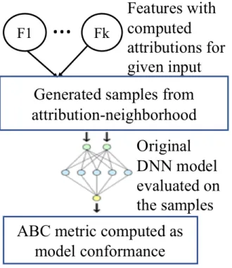
Figure 4.1: ABC complements the bottom-up inference of the original DNN model with the top-down sample generation and conformance estimation. . . 24

Figure 4.2: Attributions concentrate over few features in ImageNet. . . 26

Figure 5.1: Time taken bySAT YAfor predicting the label of adversarial and ordinary images used in CaffeNet. . . 33

Figure 5.2: Time taken bySAT YAin calculating the label for images used in GoogLeNet. The performance of both adversarial and original images have been analyzed. 33

Figure 5.3: Number of samples tested to determine the label of an original as well as an adversarial image for CaffeNet. . . 34

Figure 5.4: Number of samples tested to determine the label of an original as well as an adversarial image for GoogLeNet. . . 35

Figure 5.5: The average number of samples needed to classify an image increases as the classifier’s confidence in the label of the image decreases. . . 35

Figure 6.1: Cumulative data fraction vs. ABC for FashionMNIST and nonMNIST com-pared with MNIST. Only19%of the FashionMNIST dataset and 26% of the notMNIST dataset have a confidence higher than0.85while70%of MNIST dataset had confidence higher than0.85. . . 38

(10)

Figure 6.2: (left) Comparison of ABC metric for rotated-background-MNIST and MNIST. Rotated-background-MNIST has lower ABC confidence than MNIST. (right) ABC metric of rotated-MNIST at different angles ranging from 0 to 50 de-grees. The accuracy and confidence of the model drops with increase in rotation angle. . . 38

Figure 6.3: Comparison of attribution-based confidence metric with calibrated Platt scal-ing model for MNIST dataset rotated by 50 degrees. . . 39

Figure 6.4: Selected examples from rotated-background-MNIST with confidence show-ing quantitative analysis of ABC metric showshow-ing connection between confi-dence and interpretability. Confusing images have lower ABC values. . . 39

Figure 6.5: ABC metric for FGSM and PGD attacks on MNIST. . . 40

Figure 6.6: ABC metric for FGSM, PGD, DeepFool and CW attacks on ImageNet. . . 41

Figure 6.7: Cumulative data fraction vs. ABC metric for ImageNet and adversarial patch attacks. . . 42

Figure 6.8: Comparing ABC metric using different attribution methods: Gradients (Grad), Integrated Gradient (IG), and DeepSHAP (DS). For out of distribution ex-amples (FashionMNIST and notMNIST), results with DeepShap are slightly better than IG (which is better than Gradient). . . 43

(11)

LIST OF TABLES

Table 1.1: SAT YAcorrectly identifies95.76%of adversarial images generated by Deep-Fool against the Caffe deep learning framework for 50,000 random images. The accuracy is97.43%for adversarial versions of 50,000 randomly selected images for GoogLeNet. The accuracy for original images is within 2% of the DNN classification accuracy. . . 3

Table 3.1: Sampling the neighborhood of images at varying sampling radii. Third and fourth columns show the percentage of image correctly classified by CaffeNet and GoogleNet. Fifth and sixth column show the average number of different labels on the hyphersphere. . . 14

Table 3.2: Sampling the neighborhood of images at varying sampling radii and percent-age of those impercent-ages classified correctly for 1000 impercent-ages. . . 17

Table 5.1: Accuracy of SAT YAcompared to simple sampling approach for a sample set of 10,000 ILSVRC images. The hypersphere radius for CaffeNet was taken to be 500 units and for googleNet it was taken to be 1000 units. . . 31

(12)

Table 5.2: SAT YAcorrectly identifies 95.10%of the36882original images correctly recognized by the Caffe deep learning framework (called CaffeNet+ here) and recognizes7.53%of the13118original images not correctly recognized by Caffe (called CaffeNet- here). The accuracy is98.62% for original ver-sions of39093correctly recognized images and2.45%for original version of

10907images not correctly recognized by GoogLeNet. Here, the two classes are referred as GoogLeNet+ and GoogLeNet- respectively. . . 32

(13)

CHAPTER 1: INTRODUCTION

Artificial Intelligence systems have found applications in a variety of domains ranging from com-puter vision, speech recognition to playing games such as chess and go [6, 7, 8, 9]. The availability of big data and fast GPUs has allowed deep neural network (DNN) based AI systems to equal or sometimes exceed human-level performance on various benchmarks [10, 11, 12]. Despite these remarkable achievements, the adoption of deep learning systems in safety-critical systems is hin-dered by the inability of DNNs to handle adversarial or out-of-distribution inputs. While it is important to develop DNN models for higher accuracy, there is also a need to develop methods that characterize the limitations of these systems.

It has been shown that small perturbations to input can cause machine learning and, in particular, deep learning systems to produce incorrect answers [4, 13, 14, 2]. Computer implementations of vi-sion algorithms, including approaches based on deep learning, have been shown to be vulnerable to such adversarial attacks. These attack approaches cover a broad spectrum from a random sampling of images to the framing of an optimization problem often solved using variants of stochastic gra-dient descent. This knowledge of adversarial synthesis can be leveraged by an attacker to generate unwanted or malicious output from machine learning systems. Tampering with machine learning systems using adversarial attacks that are directly interacting with humans, such as autonomous driving, can lead to catastrophic results [15].

Machine learning systems are unable to handle out-of-distribution images. ML systems can gener-ate high confidence prediction for irrelevant input. ML systems trained only on a certain input type can still give high confidence prediction output for a compatible unrelated input and not generate any alarms. This behaviour can create problems for safety critical tasks such a medical diagno-sis where a significant change in the input can go undetected. As the adoption of ML systems is

(14)

increasing rapidly the security and robustness of these systems gain even more importance.

In this thesis, we attempt to solve the problem of adversarial attacks on deep learning systems by attempting to answer the following two questions:

1. Can we detect the adversarial nature of the input to a neural net?

2. Can we recover the correct results even when deep neural networks are exposed to adversar-ial inputs?

We introduce a new methodSAT YAthat makes progress towards answering both these questions for image classification using deep neural networks. We show that the sampling of a suitably-selected neighborhood of the input image that spans two or more classes can be used to correctly classify the input image with high probability. The Sequential Probability Ratio Test (SPRT) al-lows our approach to adaptively sample this carefully-crafted neighborhood of the input image and decide the label of a (possibly adversarial) image in a computationally efficient manner [16]. In our experimental studies, SAT YAis able to correctly classify 95.76% of adversarial images generated by the DeepFool system for the CaffeNet [17] deep learning framework. We are also able to correctly classify 97.43% of the adversarial images generated from the GoogLeNet [18] deep learning framework. For comparison the method shown in [19] detects DeepFool adversarial images with only 85-90%accuracy. This method detects50%of the original non-adversarial im-age as adversarial. In comparison, our method detects less than2%of non-adversarial images as adversarial. To the best of our knowledge,SAT YA’s accuracy on adversarial images synthesized by DeepFool [2] is the highest reported in the literature so far. Another method for detecting adver-sarial perturbations has been presented in [19], this method has been shown to work on ImageNet datasets against DeepFool perturbations. The detection probability for adversarial images has been shown to be around 85-90%for DeepFool perturbed images, though the false positive rate of

(15)

iden-tifying normal images as adversarial is around 50%. In comparisonSAT YAhas a false positive rate of less than 2%.

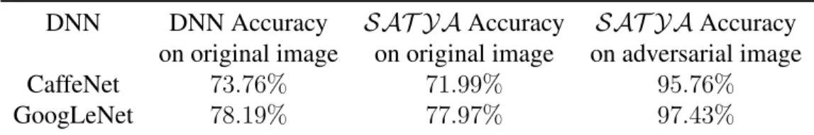
Table 1.1: SAT YA correctly identifies 95.76% of adversarial images generated by DeepFool against the Caffe deep learning framework for 50,000 random images. The accuracy is 97.43%

for adversarial versions of 50,000 randomly selected images for GoogLeNet. The accuracy for original images is within 2% of the DNN classification accuracy.

DNN DNN Accuracy SAT YAAccuracy SAT YAAccuracy on original image on original image on adversarial image CaffeNet 73.76% 71.99% 95.76%

GoogLeNet 78.19% 77.97% 97.43%

The idea that sampling can act as a defense against adversarial attacks is intuitive and straight-forward, though no concrete result of detecting adversarial examples using sampling around the space of input image has been shown in the literature. In this thesis, we show that merely sampling around the input image is enough to get good results. We show thatSAT YAgives us an improve-ment of more than 1% over this simple sampling approach. We also show thatSAT YAis more resilient to variations in the location of the adversarial image.

We then extend the sampling strategy to develop a confidence metric that can indicate when the DNN system has reached its limits and is not able to perform to the desired specification. A confidence metric would help increase trust between the human operator and the DNN system and allow further integration of DNNs in safety-critical systems such as medical diagnosis [20] and autonomous driving [21] by letting DNNs operate under standard input while giving a clear indication when the DNN prediction becomes unreliable and enabling a human or a simplex system architecture [22] to intervene. A low confidence score can also be used to detect distribution shifts or adversarial attacks. A straightforward approach to computing such a score is to use the logit values prior to the softmax layer. But this raw confidence score is poorly calibrated [23, 24] and does not correlate well with prediction accuracy. The logits reflect high confidence even on wrong

(16)

predictions over adversarial examples [25, 26, 27]. In fact, the improved accuracy in deep learning models over the last decade has been accompanied with worsening calibration of logit output to network accuracy [23] compared to earlier models [28]. It indicates overfitting in the negative log likelihood space even though DNNs avoid overfitting in the output accuracy [29]. This has motivated the development of confidence measures that use a held-out validation set for training a separate calibration model on the output of the DNNs [30, 31, 23]. But additional training or validation data may not be available with the trained machine learning (ML) model due to privacy, security or other practical constraints. Another class of confidence measures use sampling over model ensembles or training data to estimate conformance and data density [32, 33, 34]. In contrast, the focus of our work is to compute confidence for a DNN model on a given input without access to training data or the possibility of retraining a new model or model ensembles.

Figure 1.1: (From left to right) The original image with a label of yawl; masking its top 0.2%

attribution; masking its top4%of attribution; image with a banana adversarial patch [1]; masking its top 0.2% attribution; (rightmost) masking its top 4% of attribution. The classification result for the original image is robust and conforming in the neighborhood obtained by removing top positive attributions. The model predicts the original label (yawl) in the neighborhood. But the prediction changes from banana to yawl for many samples in the attribution neighborhood of the adversarial image. We observe a similar difference in conformance for the out-of-distribution examples and the adversarial examples generated by state-of-the-art digital attack methods such as DeepFool [2], PGD [3], FGSM [4] and Carlini-Wagner (CW) [5]. This observation motivates the use of conformance in the attribution-neighborhood as a confidence metric.

The confidence of a model on a given input can be measured by sampling the neighborhood of the input and observing whether the model’s output changes or conforms to the original output. But accurately estimating the conformance by sampling in the neighborhood of the input becomes

(17)

exponentially difficult with an increase in the dimension of the input [35]. We propose a novel ap-proach which samples the high-dimensional neighborhood effectively using attributions provided by methods [36, 37, 38] developed recently to improve interpretability of DNNs. In particular, we adopt the use of Shapley values with roots in cooperative game theory for computing attribu-tion. Approaches using Shapley values [38, 39] satisfy intuitively expected axiomatic properties over attributions [40]. Our attribution-based confidence metric is theoretically motivated by these axiomatic properties. The key idea is to use attributions for importance sampling in the neigh-borhood of an input. This importance sampling is more likely to select neighbors obtained by changing features with high attribution. The conformance of the machine learning model over these samples is computed as the fraction of neighbors for which the output of the model does not change. Figure 1.1 illustrates how an input that triggers incorrect responses in DNNs, such as an out-of-distribution sample or an adversarial example, does not conform in its neighborhood. Thus, the conformance of the model’s prediction in the input’s neighborhood, sampled using feature attributions, can be used as an effective measure of the confidence of the model on that input.

We make the following new contributions in the thesis.

• We propose a novel attribution-based confidence (ABC) metric computed by importance sampling in the neighborhood of a high-dimensional input using relative feature attributions, and estimating conformance of the model. It does not require access to training data or additional calibration. We mathematically motivate the proposed ABC metric using axioms on Shapley values.

• We empirically evaluate the ABC metric over MNIST and ImageNet datasets using (a) out-of-distribution data, (b) adversarial inputs generated using digital attacks such as FGSM, PGD, CW and DeepFool, and (c) physically-realizable adversarial patches and LaVAN at-tacks.

(18)

CHAPTER 2: RELATED WORK

The set of inputs to a machine learning system is significantly larger than the training set of the machine learning system. The set of inputs that the machine learning system has not been trained on can potentially confuse the machine learning system. This confusing input can be generated synthetically or obtained naturally. In this chapter, we discuss some already existing ways to generate synthetic images that fool image recognition systems. Synthetic images that fool the machine learning system are called adversarial images. We further discuss some datasets of natural images that confuse machine learning systems. These naturally existing images are classified as out-of-distribution images or natural adversarial images. Out-of-distribution images are images that are significantly different from the images that were used to train the machine learning system. Natural adversarial images are naturally occurring images that contain labels that the machine learning system was trained on but still is misclassified by the machine learning system. Finally, we discuss some methods to make the machine learning systems robust against these confusing inputs.

2.1 Synthetic Adversarial Images

Szegedy et al. were the first to show that synthetic adversarial images can easily fool deep neural networks [27]. They used box constrained L-BGFS optimization to solve the following optimiza-tion problem:

Minimizec|r|+lossf(x+r, y)subject tox+r ∈[0,1]m (2.1)

(19)

per-turbations, and the line search step size, respectively. The function f : _Rm _{→ {}₁_{· · ·}_n_} _{is the}

classifier mapping an image to a label inY ∈ {1· · ·n}. The function lossf : Rm ×Y → R+ is

the loss which maps a pair of image and label to a positive loss. In the follow up to this paper, Goodfellow et al. proposed the fast gradient sign method (FGSM) [4]. They hypothesized that neural networks are too linear, and linear perturbations to input are enough to create adversarial images. They used the sign of the loss function to generate adversarial images. The perturbationr

for this method is calculated using the following equation:

r =sgn(∇xJ(θ,x, f(x))) (2.2)

Where the variablesandθare the stepsize and model parameters, respectively. FunctionJ is the cross-entropy cost function used to train the neural network. This method can be used to generate adversarial images with a pre-specified target label or adversarial images without any pre-specified target label. The perturbation r required to generate an adversarial image with a fixed classy is calculated using the following equation: :

r =−sgn(∇xJ(θ,x, y)) (2.3)

Kurakin et al. proposed the basic iterative method (BIM) that extends the FGSM method by it-eratively applying the FGSM equation and clipping the adversarial image after each iteration to maintain a fixed distance from the original image [41]. They used the following iterative equation to generate adversarial images:

xadv₀ =x (2.4)

xadv_t₊₁ = Πx+S xadvt +αsgn(∇xJ(θ,xadvt , f(x)))

(2.5)

(20)

The functionΠx+Sis the projection function that projects an image so that the image perturbations

belong to the set of S. Kurakin et al. generated adversarial images using both FGSM and BIM methods, printed it using a color printer and then re-acquired the color prints for classification with the machine learning system. They used the term “photo transformation” to describe this proce-dure. They showed that the adversarial properties of images persist through physical printouts of images. They observed that FGSM adversarial images are more persistent to photo transformation when compared to BIM adversarial images. They hypothesized that the low robustness of BIM adversarial images to photo transformation was due to the more subtle nature of the perturbations generated by BIM. Dong et al. incorporated momentum in BIM to improve the success rate of adversarial attacks [42]. This method called the moment iterative fast gradient sign method (MI-FGSM) uses the history of past gradient directions to predict new adversarial images. The equation to calculate MI-FGSM adversarial images with decayµand accumulated gradientgis as follows:

xadv₀ =x (2.6) g0 = 0 (2.7) gt+1 =µgt+ ∇xJ(θ,xadvt , f(x)) ||∇xJ(θ,xadvt , f(x))||1 (2.8) xadv_t₊₁ =xadv_t +αsgn(gt+1) (2.9)

Madry et al. introduced the projected gradient descent (PGD) method to generate multiple adver-sarial images for adveradver-sarial training; they chose a random initial image withinS to start the BIM iteration [3]. The equation to calculate PGD adversarial images is as follows:

xadv₀ =x+swheres∈S (2.10)

xadv_t₊₁ = Πx+S xadvt +αsgn(∇xJ(θ,xadvt , f(x)))

(21)

Moosavi-Dezfooli et al. proposed the DeepFool adversarial image generation algorithm [2]. They assume that the deep neural network classifier is linear and used this assumption to calculate the minimum perturbation required to generate adversarial images. They compared their method to FGSM and show that the average perturbation required to generate adversarial images is up to 5 times lower.

Our experimental studies use the state-of-the-art DeepFool algorithm to generate adversarial exam-ples. The DeepFool algorithm is known to compute perturbations that efficiently create adversarial images for deep neural networks. To the best of our knowledge, SAT YA’s ability to defend against adversarial perturbations generated by DeepFool with more than 95% probability is new and has not been reported before in the literature.

2.2 Strategies to Make Robust AI Systems

Virtual adversarial training [43] uses a KL-divergence based robustness metric of a model against local perturbation around a data point to regularize the model. This approach has been reported to work better than ordinary adversarial training on several benchmarks, including MNIST, SVHN, and NORB.

Adversarial attacks have theoretically been shown to be more powerful than random noise per-turbations [44, 45], specifically in the context of linear classifiers. The observation of adversarial attacks in the context of high-dimensional data has been explained by formal proof demonstrating that robustness to random noise is√dtimes more than that to adversarial perturbations. Our work is motivated by this observation. Instead of feeding a single adversarial image as an input to a deep neural network, we sample a carefully-constructed neighborhood of the adversarial image and hence avoid making a decision on a single image.

(22)

Robust optimization has been used to increase the local stability of artificial neural networks [46], thereby making it harder to generate adversarial examples for such robust networks. They report up to 79.96% accuracy on adversarial images generated from the MNIST benchmark and about

65.01% accuracy on adversarial images generated from the CIFAR-10 benchmark. Our work is different from their approach as we do not seek to optimize the training of the network itself but instead seek to query enough samples so as to prevent an adversarial attack on a pre-trained classifier like GoogLeNet or CaffeNet. Of course, our approach also happens to produce better experimental results with accuracies as high as95.76%on adversarial examples for CaffeNet and

97.43%on adversarial examples for GoogLeNet.

A statistical method to detect adversarial examples has been proposed in [47], this method has been shown to work on MNIST, DREBIN and MicroRNA data with attack vectors chosen using FGSM, JSMA, SVM, and DT attacks. An impressive performance of about 100%detection in certain tests has been reported. Though no method to recover the original label of the image has been shown, one thing to note is that the data sets used in this method are significantly less complex than the ImageNet data set that we are using for our method. Another method for detecting adversarial perturbations has been presented in [19]. This method has been shown to work on ImageNet datasets against DeepFool perturbations. The detection probability for adversarial images has been shown to be around 85-90% for DeepFool perturbed images, though the false positive rate of identifying normal images as adversarial is around 50%. In comparison, SAT YA has a false positive rate of less than 2%.

2.3 Explainable AI

There has been a continued interest in interpretability of results produced by DNNs. Attribution methods assign a positive or negative value (attribution) to features of input that contribute to the

(23)

decisions made by DNNs [48, 49]. Various methods to calculate attributions have been proposed. Input-perturbation based methods occlude or perturb the input and note the change in activation of later layers to calculate attributions [50, 51]. Gradient-based methods use the gradient of the predictor function with respect to the input to calculate attributions [36, 37, 38]. Shrikumar et al. proposed the DeepLIFT method; they derived a reference activation map of individual neurons from a reference input and then used the difference between the current activation and the reference activation to calculate the contributing score of individual neurons [52]. The contributing score of individual neurons is backpropagated to the input to obtain attributions. Lundberg et al. proposed the DeepSHAP method; they used the backpropagation technique of DeepLIFT to recursively backpropagate the shapely value of individual neurons to obtain attributions [53].

(24)

CHAPTER 3: SATYA - DEFENDING AGAINST ADVERSARIAL

ATTACKS

Our approach to detecting and recovering from adversarial inputs is based on the SPRT-driven sampling of a carefully-crafted neighborhood around a (possibly adversarial) input image. In Sec-tion 3.1, we first present an intuitive method of sampling the neighborhood of input image. In Section 3.2, we improve upon the intuitive method to sample in a carefully crafted subspace and discuss its advantage over Section 3.1. The use of Wald’s sequential probability ratio test to drive an efficient exploration of this neighborhood is discussed in Section 3.3. An overview of the full method is presented in Algorithm 1.

3.1 Sampling as a Defense Against Adversarial Images

A very intuitive approach for developing a defense against adversarial images would be to sample the neighborhood of adversarial images. The underlying idea is simple: If the adversarial image happens to be adversarial only because it is carefully crafted, its neighbors may still be correctly classified by a deep neural network and hence may help void the adversarial nature of the input.

We show the arrangement of adversarial space in Figure 3.1. One important point to keep in mind is the dimensionality of the input image; even though we have shown a two-dimensional space in Figure 3.1, the search space of images has very high dimensionality. The number of dimensions

d for an input image to CaffeNet is 227x227x3, where 227 is the input dimension and 3 is the number of channels corresponding to RGB values of the input image.

(25)

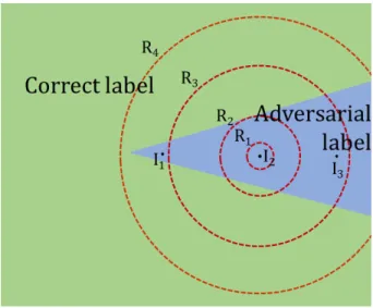
Figure 3.1: The correct non-adversarial label space is shown in green, while the adversarial space is shown in blue. The adversarial images I1, I2 and I3 are located at different locations inside

the adversarial space. The dotted lines denote hypherspheres with varying radii drawn with the imageI2 as the center. Sampling on a hyphersphere of radius R1 will give incorrect results while

sampling on a hypherphere of radiusR4 will give correct results.

For a simple sampling approach, we sample on the surface of the hypersphere centered around the input image. We use the sampling method described in [54] to generate uniformly distributed points on the surface of ad-dimensional hyphersphere. To generate a random pointPi, we generate

d random numbers ri0, ri1. . . rid fromd independent standard normal distribution with µ= 0, σ

= 1 and d = x×y×c, where xand y are the dimensions of the image and cis the number of channels in the image. Let Gi = [ri0 ri1 . . . rid], then the random point Pi on the surface of

d-dimensional hyphersphere with radiusRis given by Equation 3.1. This equation is implemented by the functionN in Algorithm 1.

Pi =

R

kGik

(26)

If an adversarial image is deep inside the adversarial space, sampling on low radius hypherspheres will only give adversarial samples as shown byR1 andR2 in Figure 3.1. An image likeI3 that is

further inside the adversarial space will require a larger hyphersphere radius to give correct samples when compared to the imageI1. We test the accuracy of detection at various radii for 1000 sample

images for both CaffeNet and GoogLeNet; we show the results in Table 3.1. The performance of CaffeNet is optimal for a radius of 500 units where it reaches the peak accuracy of 92.6%. The performance of GoogLeNet is optimal at 1000 units where the accuracy is 97.0%. We suspect that this difference in peak accuracy at different radii is due to the generally different performance of DeepFool on these two different networks. In the case of CaffeNet, DeepFool might be creating adversarial images closer to the boundary of the adversarial space whereas for GoogLeNet the adversarial image might be further inside the adversarial space.

Table 3.1: Sampling the neighborhood of images at varying sampling radii. Third and fourth columns show the percentage of image correctly classified by CaffeNet and GoogleNet. Fifth and sixth column show the average number of different labels on the hyphersphere.

Hyperhsphere Correct Correct Average Number Average Number Index radius Percentage Percentage of Labels of Labels

CaffeNet GoogLeNet CaffeNet GoogLeNet

1 50 5.7% 6.7% 1.94 1.91 2 100 21.9% 8.0% 1.80 1.71 3 200 58.3% 33.2% 1.60 1.48 4 500 92.6% 94.0% 1.43 1.31 5 1000 90.8% 97.0% 1.36 1.27 6 1500 89.2% 96.3% 1.38 1.29 7 2000 86.4% 94.5% 1.45 1.34 8 3000 79.2% 91.0% 1.65 1.49 9 5000 64.1% 83.7% 2.31 2.06

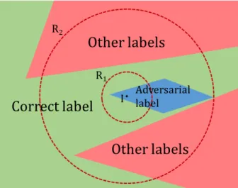
One trend that we observe in Table 3.1 is the decline in accuracy as the radius of the hypersphere increases beyond 1500 units. Hypherspheres with higher radii have larger volume and can accom-modate samples of multiple labels as shown in Figure 3.2. Multiple labels on the hyphersphere can decrease the chance of the correct label having the maximum number of samples. This hypothesis

(27)

is confirmed by the fact that we observe an increase in the average number of labels on the hypher-sphere as the radius increases from 1500 units. One natural conclusion from these experimental observations is that an algorithmic approach to defend against adversarial attacks should construct a consistent search space unaffected by the position of the adversarial image inside the adversarial space.

Figure 3.2: Sampling around the imageI. A low radiusR1 will give correct results, while a very

high radiusR2 is likely to give incorrect results.

3.2 Constructing a Suitable Sample Space

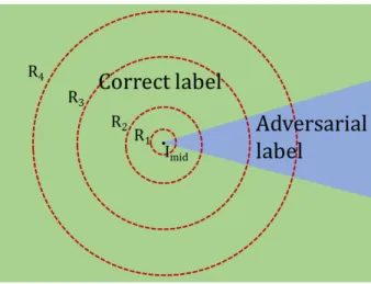
One suitable candidate for a consistent sampling space is the neighborhood of an image that is on the boundary between the correct non-adversarial space and the adversarial space. This image is shown as Imid in Figure 3.3. The location of Imid reduces the need for finding the optimal

hyphersphere radius for sampling. We present the procedure to calculate the image Imid in this

section. We iterate that the figures shown here are a simplification of the more complicated high dimensional space.

(28)

Figure 3.3: Sampling around the imageImid at the border of the space of correct non-adversarial

label and adversarial label. Sampling on most hyphersphere radii will give correct results.

Given an input imageI and a deep neural network (DNN) classifier C, SAT YAfirst calculates the best classification labell1for the imageI. It also computes the second-best classification label

l2 for the same image. For an adversarial image generate by DeepFool, the second labell2 is the

correct label. Similarly for the non adversarial image, the label l2 is the incorrect label and is

the label of the adversarial space. We generate the image Imid using the gradient generated by

the backpropagation function of the DNN. The error functionE(I, l)of the classifier C gives the backpropagated error at the input layer with the input imageI and the correct labell. At each step

j of the iteration, for an input imageIj the errorE(Ij, l2)of the input layer of DNN is generated

by assumingl2as the correct label of the image. The new imageIj+1is generated using the update

Ij+1 ₌_Ij₊_E₍_Ij_{, l}

2). Each iteration generates an image with higher confidence ofl2. We continue

adding E(Ij_{, l}

2) until at iteration k, l2 is the highest confidence label of the image. The image

Ik _{has the label} _l

2 and the image Ik−1 has the label l1. The image Imid is calculated by doing

a binary search between the images Ik andIk−1 to get an image on the separating boundary of the two labelsl1 andl2. The algorithm then samples images on the surface of ann-dimensional

(29)

The results of sampling with various radii for 1000 images is shown in Table 3.2. For both CaffeNet and GoogLeNet, good accuracy is obtained at the smallest sampled radius of 50 units. We note that the accuracy ofSAT YAis better than simple sampling around the adversarial image. We revisit this comparison with higher number of samples in the experimental section. We can also note that there is less variation between the accuracy at different hyphersphere radii forSAT YA. In Table 3.1 the standard deviation for CaffeNet is 29.98 whereas the standard deviation in Table 3.2 is 10.16. Similarly for GoogLeNet, the standard deviation in Table 3.1 is 37.05 where as it is 4.34 for Table 3.2. This simple metric shows us that the results obtained fromSAT YAis more resilient to variations in the location of the adversarial image.

In our current implementation, we have only considered the top-2 labelsl1andl2 for deciding the

correct label of the image. The limitation of top-2 labels works in the case of DeepFool as the adversarial attack algorithm works gradually towards an adversarial label and the algorithm termi-nates at the first instance of a wrong label thus leaving the correct label asl2. For implementing a

top-n variant of this algorithm, a competition between the top-n labels can be organized and the winner declared as the current label.

Table 3.2: Sampling the neighborhood of images at varying sampling radii and percentage of those images classified correctly for 1000 images.

Hypersphere Correct Correct Correct Correct Index radius Prediction Percentage Prediction Percentage

CaffeNet CaffeNet GoogLeNet GoogLeNet

1 50 974 97.4% 970 97.0 % 2 100 963 96.3 % 973 97.3 % 3 200 952 95.2 % 974 97.4 % 4 500 926 92.6 % 977 97.7% 5 1000 896 89.6 % 963 96.3 % 6 1500 886 88.6 % 956 95.6 % 7 2000 858 85.8 % 941 94.1 % 8 3000 783 78.3% 915 91.5 % 9 5000 635 63.5 % 834 83.4 %

(30)

Algorithm 1SAT YAAdversarial Image Classification

Input: ImageI, Set of labelsL, Deep Neural Network Classifier C, Input layer error function

of classifierE, Type I/II errore, Maximum number of samples N, Indifference region[p0, p1],

Maximum number of iterations for searching middle imageM, Sampling radiusR

Output:Classification label for imageI

l1 =arg max

l∈L

C(I, l) .Find best label for imageI

l2 =arg max

l∈{L\l1}

C(I, l) .Find second-best label forI

lc=l1,I1 =I,I2 =I,m = 0,n = 0,s= 0 while lc6=l2 do I1 =I2 I2 =I2+E(l2) lc=C(I2) end while

.Perform binary search to compute the boundary betweenl1andl2

Imid =B(I1, I2)

.Compute SPRT stopping criteria for Type I/II error

Smin = log(₁₋e_e),Smax = log(1−_ee)

repeat

n =n+ 1 .Increment total number of samples

J = samplei.i.d. fromN(Imid, R)

ifC(J) =l2 then

s=s+ 1 .Increment no. of successful samples

end if

.Update Sequential Probability Ratio

S =log ps 1(1−p1)n−s ps 0(1−p0)n−s

untilS < SminorS > Smaxorn≥N

ifs > n−sthen

print Class label: l2

else

print Class label: l1

end if

3.3 Statistical Hypothesis Testing

The sampling neighborhood around the transition imageImid constructed in the previous

subsec-tion is quantitatively different for different input images. For adversarial images generated from images that were correctly recognized by the DNN classifierC with high-confidence, we find that

(31)

the sampling neighborhood contains an overwhelming majority of images that are correctly la-beled by the DNN classifierC. On the other hand, the sampling neighborhood only contains a thin majority of images correctly labeled by the DNN classifierC if the original image was correctly classified by the classifier with a very low confidence.

SAT YAuses the Sequential Probability Ratio Test (SPRT) to adaptively sample the neighborhood constructed in the previous subsection [16]. The test rejects one of the following two hypotheses:

Null Hypothesis: Cassigns the labell2to images in the neighborhood ofImidwith probability more

thanp1

Alternate Hypothesis:Cassigns the labell2to images in the neighborhood ofImidwith probability

less thanp0

The user specifies an indifference region[p0, p1], Type I/II errore and the maximum number of

samples to be obtained N. SPRT then samples the neighborhood recording the total number of images sampled (n) and the number of images (s) labeled by the classifier as l2. Using these

inputs, SPRT computes the likelihood ratio:

ps

1(1−p1)n−s

ps

0(1−p0)n−s

If the likelihood ratio falls below a threshold derived from the Type I/II error, SPRT rejects the null hypothesis. If the likelihood ratio exceeds a threshold, SPRT rejects the alternate hypothesis.

If the probability of sampling an image with the labell2is more thanp1, the algorithm will produce

this label with probability1−e. For example, ifp1 = 0.51ande = 0.01, our algorithm produces

this label with 99% accuracy if the sampling neighborhood has at least 51% correctly labeled images. Of course, greater accuracy can be achieved by reducing the Type I/II error and by setting

(32)

the value ofp1to0.5 +for a small >0. However, this comes at the expense of a larger number

of samples needed to reach a conclusion.

In Figures 5.3 and 5.4, we show how the number of samples required by our statistical hypothesis testing algorithm can vary widely among different input images. In particular, adversarial images that are generated from images for which the DNN classifier C was making a correct but low-confidence prediction tend to require larger number of samples. Figure 5.5 shows that the number of samples required to disambiguate an adversarial image generated from an original image clas-sified with confidence between 0.4 and 0.6 is more than 5 times the number of samples required for a high-confidence (0.8-1.0) prediction. Thus, the SPRT-driven adaptive sampling is critical to ensure an efficient performance ofSAT YA.

(33)

CHAPTER 4: ATTRIBUTION-BASED CONFIDENCE METRIC

Our proposed confidence metric (ABC) is closely related to the literature on confidence metrics, attribution methods and techniques for adversarial attacks and defenses for DNNs.

Confidence metrics: The need for confidence metric to reflect the uncertainty in the output of

machine learning models was recognized very early in the literature [31, 30]. The high accuracy but brittleness of deep learning models has revived interest in defining confidence metrics that reflect the accuracy of the model. DNNs are not well-calibrated [23, 32, 33] and so, the straightforward use of logit layer before softmax as a confidence measure is not reliable. Several post-processing based confidence metrics have been proposed in the literature which can be grouped into three classes:

• Calibration models trained using held-out validation set: [31] proposed a parametric ap-proach where the logits are used as features to learn a calibration model from a held-out validation set. An example calibration model is qi = maxkσ(W zi +b)k where zi are the

logits, σ is the standard sigmoid function, k denotes a class, (·)k _{denotes the} _k_{-th element}

of a vector, and W, b are parameters [28]. Temperature scaling is a special case of Platt scaling with a single parameter. Nonparametric learning of calibration models from held-out validation data has been also proposed in the form of histogram binning [55], isotonic regression [56] and Bayesian binning [57].

• Model ensemble approaches: [58] use ensembles of networks to obtain uncertainty esti-mates. Bayesian neural networks [30, 59] return a probability distribution over outputs as an alternative way to represent model uncertainty. Sampling models by dropping nodes in a DNN has been shown to estimate probability distribution over all models [60].

(34)

• Training-set-based uncertainty estimation: [33] compute the trust score on deeper layers of a DNN than input to avoid the high-dimensionality of inputs. They propose a trust score that measures the conformance between the classifer and a modified nearest-neighbor classifier on the testing example. [32] usek-nearest neighbors regression using training set on the in-termediate representations of the network which showed enhanced robustness to adversarial attacks and leads to better calibrated uncertainty estimates.

In contrast to these approaches, ABC metric only needs the trained model at inference time, and does not require training data, separate held-out validation data or training a model ensemble.

DNN robustness, adversarial inputs and defense: Szegedy et al. used L-BFGS method to

gen-erate adversarial examples [27]. Goodfellow et al. proposed a fast gradient sign method (FGSM) to generate faster adversarial images as compared to the L-BFGS method; this method performed only a one-step gradient update at each pixel along the direction of the gradient’s sign [4]. Rozsa et al. replaced the sign of the gradients with raw gradients [61]. Dong et al. applied momentum to FGSM [42], and Kurakin et al. further extended FGSM to a targeted attack [41]. A number of adversarial example generation techniques [2, 3, 5] are now available in tools such as Clever-hans [62] which we use in our experiments. In addition to digital attacks, we also study how the proposed ABC metric measures uncertainty on physically realizable attacks in form of patches or stickers [1, 63]. Further, the adversarial examples have been shown to transfer [64, 65] across models making them agnostic to availability of model parameters and effective against even en-semble approaches. Efforts over the last few years to defend against adversarial attacks have met with limited success. While approaches such as logit pairing [66], defensive distillation [67], manifold-based defense [68, 69], and adversarial training methods that exploit knowledge of the specific attack [70], have shown effectiveness against particular attack methods, more principled techniques such as robust optimization [71, 72, 3] and formal methods [73] are limited to

(35)

pertur-bations with boundedLp norm. Schott et al. present an insightful study of the state of the art on

attacks and defenses [74], and proposes an analysis by synthesis defense. This arms race between attacks and defenses are not limited to computer vision, but extend to audio and natural language processing. Schonner et al. were able to fool the state-of-the-art speech recognition system Kaldi using audio noise that were barely distinguishable to a human listener [75]. Qin et al. then im-proved the construction of adversarial examples to create audio noise that was imperceptible to humans [76].

Our approach to addressing the challenge of DNN’s susceptibility to adversarial examples using ABC metric differs from the majority of prior work in that it measures confidence of a model’s prediction to characterize the credibility of a DNN on a given input instead of attempting to classify all legitimate and malicious inputs correctly or make particular adversarial strategies fail.

Model interpretability and attribution methods: A number of explanation techniques [39, 38,

48, 49, 77, 78] have been recently proposed in the literature that either find a complete logical explanation or just the relevant features or assign quantitative importance (attributions) to input features for a given model decision. Many of these methods are based on the gradient of the predictor function with respect to the input [36, 37, 38]. Different attribution methods are compared in [79]. The sensitivity of these attributions to perturbations in the input are studied in [80], and indicate the potential of adversarial attacks on the proposed and other existing confidence metrics. But attacking the model and its confidence measure is more difficult than just attacking the model. This motivates the use of ABC metric to measure confidence. The brittleness of learning has been related to anti-causal direction of learning [81]. We observe that the wrong decisions for out-of-distribution and adversarial inputs often hinge on a relatively small concentrated set of high attribution features, and thus, mutating these features and generating samples in the neighborhood of the original input is an effective top-down inference that is robust to adversarial attacks. In recent work [82], we have demonstrated the use of attributions for detecting adversarial examples.

(36)

Figure 4.1: ABC complements the bottom-up inference of the original DNN model with the top-down sample generation and conformance estimation.

4.1 ABC Metric Motivation

Motivation: The proposed ABC metric is motivated by Dual Process Theory [83, 84] and

Kah-neman’s decomposition [85] of cognition into System 1, or the intuitive system, and System 2, or the deliberate system. The original DNN model represents the bottom-up System 1, and the ABC metric computation is a deliberative top-down System 2 that uses the attributions in System 1 to generate new samples in the neighborhood of the original input. [81] argue that causal mechanisms are typically continuous but most learning problems such as classification are anti-causal. The lack of resilience to adversarial examples is hypothesized to be the result of learning in an anti-causal direction. Combining both the anti-causal System 1 DNN model and the attribution-driven System 2 that computes the ABC metric creates a relatively more resilient cognition model. ABC metric

(37)

uses the attribution over features for the decision of a machine learning model on a given input to construct a generator that can sample the attribution-neighborhood of the input and observe the conformance of the model in this neighborhood. While learning is still in the anti-causal direction, ABC adds causal deliberative System 2 that reasons in the forward generative direction to evaluate the conformance of the model.

Computational challenge:The computation of ABC metric of an ML model on an input requires

accurately determining conformance by sampling in the neighborhood of high-dimensional in-puts. This can be addressed by sampling over lower-dimensional intermediate or output layers of a DNN [32, 30], or relying on topological and manifold-based data analysis [33]. But these methods require training data that may not always be available at inference time. ABC addresses this chal-lenge by biasing our sampling using the quantitative attribution obtained via Shapley values [38]. Deep learning models demonstrate a concentration of features, that is, few features have relatively very high attributions for any decision. Figure 4.2 illustrates feature concentration for ImageNet where the attribution is computed via Integrated Gradients [38]. Sampling over low attribution features will likely lead to no change in the label. Low attribution indicates that model is equiv-ariantalong these features. By focusing on high attribution features during sampling, our method can efficiently sample even high-dimensional input spaces to obtain a conservative estimate of the confidence score.

ABC uses feature attributions for dimensionality reduction followed by importance sampling in the reduced-dimensional neighborhood of the input to estimate DNN model’s conformance. But unlike typical principal component analysis techniques that search for globally important features, we identify features that are locally relevant for the given input. This enables our approach to conservatively approximate conformance measure of a model in even high-dimensional input’s neighborhood and, thus, efficiently compute the ABC confidence metric of the model on the input.

(38)

0

20

40

60

80

100

0

1

2

3

4

5

·

10

−2

Features Percentile

Attrib

ution

Magnitude

80

85

90

95

100

0

1

2

3

4

5

·

10

−2

Percentile (Magnifying 80 to 100 range)

Figure 4.2: Attributions concentrate over few features in ImageNet.

4.2 ABC Algorithm

In this section, we theoretically motivate the proposed ABC metric and present an algorithm for its computation. Attribution methods using Shapley values often employ the notion of a baseline inputxb_{; for example, the all dark image can be the baseline for images. The baseline can also be}

a set of random inputs where attribution is computed as an expected value. Let the attribution for thej-th feature and output labelibeAi

j(x). The attribution for the j-th input feature depends on

the complete inputxand not just xj. The treatment for each logit is similar, and so, we drop the

logit/class and denote the network output simply asF(·)and attribution asAj(x). For simplicity,

we use the baseline inputxb _{= 0}_{for computing attributions. We make the following two}

assump-tions on the DNN model and the attribuassump-tions, which reflect the fact that the model is well-trained and the attribution method is well-founded:

(39)

at-tribution methods based on Shapley values such as Integrated Gradient [38] which define attribution as the path integral of the gradients of the DNN output with respect to that feature along the path from the baselinexbto the inputx, that is,

Ai

j(x) = (xj−xbj)×

Z 1

α=0

∂jFi(xb+α(x−xb))dα (4.1)

where the gradient of i-th logit output of the model along the j-th feature is denoted by

∂jFi(·).

• Attributions are complete i.e. the following is true for any inputxand the baseline inputxb:

F(x)− F(xb) = n

X

k=1

Ak(x)wherexhasnfeatures. (4.2)

Shapley value methods such as Integrated Gradient and DeepShap [38, 39] satisfy this axiom too.

We first establish a relationship between attributions and the sensitivity of the model’s output to change in an input feature. This is useful in attribution-based dimensionality reduction of a high-dimensionalxand defining its attribution-neighborhood.

Theorem 1 The sensitivity of the outputF(x)with respect to an input featurexj in the

neighbor-hood ofxis approximately the ratio of the attributionAj(x)to the value of that featurexj, that is,

Aj(x)

xj .

Given an inputxand its neighborx0 =x+δx, we can use Taylor series expansion to express the outputF(x0)as: F(x0) =F(x) + n X k=1 (∂F(x) ∂xk δxk) + max k=1,...,nO(δx 2 k). (4.3)

(40)

Assuming the completeness of attribution over the features of the inputx0, we obtain the following: F(x0)− F(xb) = n X k=1 Ak(x0). (4.4)

Subtracting Equation 4.2 from 4.4, we can eliminate the baseline inputxb _{and use Taylor series to}

obtain: F(x0)− F(x) = n X k=1 (Ak(x0)− Ak(x)) = n X k=1 ∂Ak(x) ∂xk δxk + max k=1,...,nO(δx 2 k) . (4.5)

While computing conformance, we sample only neighbors of the input and so we can drop the higher order terms in both Equations 4.5 and 4.3. These equations hold for all neighbors including those which differ in only one of the featuresxj and so, we can conclude that the sensitivity of the

model with respect to a featurexj is ∂Aj(x)

∂xj .

Taking the derivative of Equation 4.1 on both sides with respect to feature xj and ignoring the

non-linear attribution terms, we obtain the following:

∂Aj(x) ∂xj = Z 1 α=0 ∂F(xb+α(x−xb)) ∂xj dα+xj ∂ ∂xj Z 1 α=0 ∂F(xb+α(x−xb)) ∂xj dα = Z 1 α=0 ∂F(xb₊_α₍_x₋_xb₎₎ ∂xj dα+xj Z 1 α=0 ∂2_F₍_xb₊_α₍_x₋_xb₎₎ ∂x2 j dα ≈ Z 1 α=0 ∂F(xb₊_α₍_x₋_xb₎₎ ∂xj dα = Aj(x) xj

from Eqn. 4.1 with baseline featurexb_j = 0.

(4.6)

Thus, we have shown that the sensitivity of the model’s output with respect to an input feature in the neighborhood of the input is approximately given by the ratio of the attribution for that input feature

(41)

to the value of that feature. Note that Aj(x)

xj does not vanish even when the traditional sensitivity

given by ∂F_∂_x(x)

j vanishes exploiting the non-saturating nature of Shapley value attributions. The

model is almost equivariant with respect to features with lowAj(x)/xj and, thus, the

attribution-neighborhood is constructed by mutating features with highAj(x)/xj. The overall algorithm for

computing ABC metric of a DNN model on an input is as follows.

Algorithm 2Evaluate ABC confidence metricc(F,x)of machine learning modelF on inputx

Input: ModelF, Inputxwith featuresx1,x2, . . .xn, Sample sizeS

Output: ABC metricc(F,x)

1: A₁, . . .An←Attributions of featuresx1,x2, . . .xnfrom inputx

2: i← F(x) .Obtain model prediction

3: forj = 1tondo 4: P(xj)← Aj/xj Pn k=1Ak/xk 5: end for

6: GenerateSsamples by mutating featurexj of inputxto baselinexbj with probabilityP(xj)

7: Obtain the output of the model on theS samples.

8: c(F,x)←Sconform/Swhere model’s output onSconform samples isi

(42)

CHAPTER 5: SATYA - EXPERIMENTAL RESULTS

We evaluated SAT YA on 50,000 images from the ILSVRC2013 training dataset [86] for both the CaffeNet [17] and the GoogLeNet [18] deep learning frameworks. Adversarial versions of these images were created using the state-of-the-art DeepFool [2] adversarial attack system. In our experiments, we have used the following parameters for the SAT YA algorithm: Type I/II error e = 0.000001, maximum number of samples N = 2000, indifference regions p0 = 0.47

andp1 = 0.53, maximum number of iterations for searching the transition imageImid M = 500

and hyphersphere radius for samplingR = 200units. Our experiments were carried on a 16GB Intel(R) Core(TM) i7-4770K CPU @ 3.50GHz workstation with an NVIDIA GeForce GTX 780 GPU. Our experimental evaluation has four goals:

1. How well does SAT YA perform on the adversarial images generated by the DeepFool algorithm working with CaffeNet and on adversarial images generated for GoogLeNet? 2. What is the impact ofSAT YAon original non-adversarial benchmarks?

3. How is the runtime performance ofSAT YA?

4. Does the runtime of our approach vary significantly depending on the image being investi-gated?

5.1 Accuracy on Adversarial Images

SAT YAcorrectly identifies more than 95%of all the adversarial images generated for both the CaffeNet deep neural network and the GoogLeNet deep learning framework. The results for the execution on 50,000 ILSVRC images is shown in Table 1.1. The hyphersphere radius for sampling

(43)

was taken to be 200 units for both CaffeNet and GoogLeNet. The accuracy of detection of the correct label was 95.76% for CaffeNet and 97.43% for googleNet.

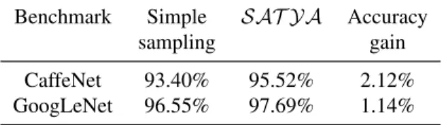
To compare SAT YAwith simple sampling approch around input adversarial image we ran the benchmark on the same set of 10,000 random ILSVRC images. The hyphersphere radius for best accuracy was 500 units for CaffeNet and 1000 units for GoogLeNet. We show the experimental results in Table 5.1. We can see that an accuracy gain of 2.12% for CaffeNet and 1.14% for googleNet was achieved usingSAT YA.

Table 5.1: Accuracy ofSAT YAcompared to simple sampling approach for a sample set of 10,000 ILSVRC images. The hypersphere radius for CaffeNet was taken to be 500 units and for googleNet it was taken to be 1000 units.

Benchmark Simple SAT YA Accuracy sampling gain CaffeNet 93.40% 95.52% 2.12% GoogLeNet 96.55% 97.69% 1.14%

5.2 Accuracy on Original Unperturbed Images

While SAT YA’s performance on adversarial images is very good, it would not be a useful al-gorithm if its performance on non-adversarial images turned out to be poor. SAT YAperforms very well even on original adversarial images. The accuracy of CaffeNet on the original non-adversarial image is 73.76% while the accuracy ofSAT YAon CaffeNet is 71.99%. The accuracy of GoogLeNet on the original non-adversarial image is 78.19% while the accuracy ofSAT YA

on original image is 77.54%. We can see that the underlying detection algorithms perform only slightly better thanSAT YA. The breakup for images correctly and incorrectly classified by Caf-feNet is given in Table 5.2. We can see thatSAT YA correctly classifies 7.53% of image orig-inally incorrectly classified by CaffeNet and 2.45% of image origorig-inally incorrectly classified by GoogLeNet.

(44)

Table 5.2: SAT YAcorrectly identifies95.10%of the36882original images correctly recognized by the Caffe deep learning framework (called CaffeNet+ here) and recognizes7.53%of the13118

original images not correctly recognized by Caffe (called CaffeNet- here). The accuracy is98.62%

for original versions of39093correctly recognized images and2.45%for original version of10907

images not correctly recognized by GoogLeNet. Here, the two classes are referred as GoogLeNet+ and GoogLeNet- respectively.

Prediction Correct Benchmark Wrong Correct Percentage

CaffeNet+ 1808 35074 95.10% CaffeNet- 12199 919 7.53% GoogLeNet+ 540 38553 98.62% GoogLeNet- 10646 261 2.45%

5.3 Runtime Performance

The time required by SAT YA to analyze both original and adversarial images for CaffeNet is shown in Figure 5.1 and for GoogLeNet is shown in Figure 5.2. The runtime performance of

SAT YAis acceptable for high-fidelity applications like cyber-physical systems. An overwhelm-ing majority of the images were analyzed by SAT YA within 4 seconds. We should note that the availability of enough parallel computational resource can be used to speed up SAT YA to match the runtime performance of the underlying classifier by using massively parallel calls from

SAT YAto the underlying classifier such as CaffeNet or GoogLeNet.

SAT YAcorrectly recognizes about91%of the adversarial images and70%of the original images within 4 seconds on our single GPU machine with only sequential calls to the DNN CaffeNet classifier. The worst case runtime of our approach on adversarial images is 22 seconds for the CaffeNet deep neural network.

The performance ofSAT YAon images from the GoogLeNet is qualitatively similar to the results on CaffeNet. About98%of the adversarial images and75%of the original images can be analyzed

(45)

within 4 seconds. The worst case runtime of SAT YA on adversarial images is 27seconds for GoogLeNet. 0–2 2–4 4–6 6–8 8–10 10+ 0 200 400 600 800 seconds number of images

(a) Adversarial Images

0–2 2–4 4–6 6–8 8–10 10+ 0 100 200 300 400 seconds number of images (b) Original Images

Figure 5.1: Time taken by SAT YAfor predicting the label of adversarial and ordinary images used in CaffeNet. 0–2 2–4 4–6 6–8 8–10 10+ 0 200 400 600 seconds number of images

0–2 2–4 4–6 6–8 8–10 10+ 0 200 400 600 800 seconds number of images (b) Original Images

Figure 5.2: Time taken bySAT YAin calculating the label for images used in GoogLeNet. The performance of both adversarial and original images have been analyzed.

(46)

5.4 Dependence of Performance on the Confidence of Classification

The performance of SAT YA depends upon the number of images sampled by the sequential probability ratio test. In Figure 5.3, we illustrate the number of samples required by SAT YA

while analyzing original and adversarial images for CaffeNet. About50%of the adversarial images can be analyzed by studying only200samples. Similarly, about55%of the original images can be classified by analyzing only200samples. Only a small fraction of images require more than1,000

samples. 0–200 200–400 400–600 600–800 800–1000 1000+ 0 100 200 300 400 500 samples number of images

(a) Perturbed Images

0–200 200–400 400–600 600–800 800–1000 1000+ 0 200 400 600 samples number of images (b) Original Images

Figure 5.3: Number of samples tested to determine the label of an original as well as an adversarial image for CaffeNet.

Figure 5.4 shows the number of samples required by original and adversarial images for the GoogLeNet deep learning framework. About 80% of the perturbed images and more than 75%

of the original images were analyzed by sampling fewer than 200 samples. In the light of this variation in number of samples for a small fraction of the images, a natural question that arises is the source of this variability. Using Figures 5.5 we establish an empirical relationship between the

(47)

number of samples required to disambiguate an image and the confidence with which the classifier assigns a label to the image.

0–200 200–400 400–600 600–800 800–1000 1000+ 0 200 400 600 800 samples number of images

0–200 200–400 400–600 600–800 800–1000 1000+ 0 200 400 600 800 samples number of images (b) Original Images

Figure 5.4: Number of samples tested to determine the label of an original as well as an adversarial image for GoogLeNet.

1.0–0.8 0.8–0.6 0.6–0.4 0.4–0.2 0.2–0.0 0 200 400 600 800 confidence av erage number of samples (a) CaffeNet 1.0–0.8 0.8–0.6 0.6–0.4 0.4–0.2 0.2–0.0 0 200 400 600 800 confidence av erage number of samples (b) GoogLeNet

Figure 5.5: The average number of samples needed to classify an image increases as the classifier’s confidence in the label of the image decreases.

(48)

We observed qualitatively similar results for adversarial images generated for the GoogLeNet deep learning classifier. Adversarial inputs generated using images that were assigned high-confidence labels by GoogLeNet (0.6 or more) were easily labeled bySAT YAusing fewer than 300 sam-ples. The fact that SAT YA is able to recover the labels of adversarial inputs generated from confidence images is extremely desirable. Such a performance behavior implies that high-confidence predictions from a classifier may be difficult to distort in a manner where they cannot be recovered bySAT YAand other defensive approaches.

(49)

CHAPTER 6: ABC - EXPERIMENTAL RESULTS

We evaluate the attribition-based confidence metric on out-of-distribution data and adversarial at-tacks. All experiments were conducted on a 8 core IntelRCoreTMi9-9900K 3.60GHz CPU with

NVIDIA Titan RTX Graphics and 32 GB RAM.

6.1 Out-of-distribution Images

We computed ABC metric for MNIST, MNIST [87] with rotation and background, notMNIST [88], and FashionMNIST [89] datasets. The DNN model was trained on MNIST images. Input com-patible images such as rotated MNIST, notMNIST and FashionMNIST act as out-of-distribution datasets for the DNN model. In our experiments we observed that the average ABC metric of MNIST dataset is higher than the average ABC metric of out-of-distribution datasets. Only19% of the FashionMNIST dataset and 26% of the notMNIST dataset have a confidence higher than 0.85 while 70% of MNIST dataset had confidence higher than 0.85. The results of the experiments are shown in Figure 6.1

We compare the predicted accuracy vs confidence below to evaluate how well the attribution-based confidence metric reflects the reduced accuracy on the rotated MNIST dataset with a background image [90]. The dataset has MNIST images randomly rotated by0 to 2π, and with a randomly selected black/white background image. The accuracy and confidence of the model drops with in-crease in rotation angle (from0to50degrees) and decrease in accuracy as illustrated in Figure 6.2. The three examples show how the ABC metric reflects the confusability of inputs. We compare the ABC metric with a trained calibrated scaling model in Figure 6.3.

(50)

0 0.2 0.4 0.6 0.8 1 0 0.2 0.4 0.6 0.8 1 Attribution-based Confidence Cumulati v e Fraction of Data Fashion-MNIST MNIST 0 0.2 0.4 0.6 0.8 1 0 0.2 0.4 0.6 0.8 1 Attribution-based Confidence Cumulati v e Fraction of Data notMNIST MNIST

Figure 6.1: Cumulative data fraction vs. ABC for FashionMNIST and nonMNIST compared with MNIST. Only19%of the FashionMNIST dataset and 26% of the notMNIST dataset have a confi-dence higher than0.85while70%of MNIST dataset had confidence higher than0.85.

Figure 6.2: (left) Comparison of ABC metric for rotated-background-MNIST and MNIST. Rotated-background-MNIST has lower ABC confidence than MNIST. (right) ABC metric of rotated-MNIST at different angles ranging from 0 to 50 degrees. The accuracy and confidence of the model drops with increase in rotation angle.

(51)

0 0.2 0.4 0.6 0.8 1 0 0.2 0.4 0.6 0.8 1

Confidence on MNIST Rotated by 50 degrees

Fraction

of

Data

Calibrated Scaling Attribution-based Confidence

Figure 6.3: Comparison of attribution-based confidence metric with calibrated Platt scaling model for MNIST dataset rotated by 50 degrees.

Figure 6.4: Selected examples from rotated-background-MNIST with confidence showing quanti-tative analysis of ABC metric showing connection between confidence and interpretability. Con-fusing images have lower ABC values.

(52)

6.2 Adversarial Images

We calculated the ABC metric for both digital and physical adversarial images. Figure 6.5 il-lustrates how the decreased ABC metric reflects the decrease in accuracy on MNIST adversarial examples. The accuracy with PGD attack drops close to zero, and so, we only plot the fraction of data with different confidence levels. We calculated ImageNet adversarial images using FGSM, PGD, CW, and DeepFool attacks. Figure 6.6 illustrates how the ABC metric reflects the decrease in accuracy under adversarial attack.

We applied physically realizable adversarial patch [1] and LaVAN [63] attacks on 1000 images from ImageNet. For the adversarial patch attack, we used a patch size of 25%for two patch types: banana and toaster. For LaVAN, we used a baseball patch of size 50× 50 pixels. Figure 6.7 illustrates how the ABC metric is low for most of the adversarial examples reflecting the decrease in the accuracy of the model.

0 0.2 0.4 0.6 0.8 1 0 0.5 1 Attribution-based Confidence Cumulati v e Fraction of Data FGSM MNIST 0 0.2 0.4 0.6 0.8 1 0 0.5 1 Attribution-based Confidence Cumulati v e Fraction of Data PGD MNIST