Automated elephant detection and classification from aerial infrared and colour images using deep learning

(1)

Automated elephant detection and classification from aerial

infrared and colour images using deep learning

by

Jacques Charles Marais

Thesis presented in partial fulfilment of the requirements for the degree of

Master of Science in Applied Mathematics in the Faculty of Science at

Stellenbosch University

Supervisor: Dr WH Brink

(2)

Declaration

By submitting this thesis electronically, I declare that the entirety of the work contained therein is my own, original work, that I am the sole author thereof (save to the extent explicitly otherwise stated), that reproduction and publication thereof by Stellenbosch University will not infringe any third party rights and that I have not previously in its entirety or in part submitted it for obtaining any qualification.

March 2018

Date: . . . .

i

(3)

Abstract

In this study we attempt to detect and classify elephants in aerial images using deep learning. This is not a trivial task even for a human since elephants naturally blend in with their surround-ings, making it a challenging and meaningful problem to solve. Possible applications of this work extend into general animal conservation and search-and-rescue operations, with natural exten-sion to satellite imagery as input source.

We create a region proposal algorithm that relies on digital image processing techniques and morphological operations on infrared images that correspond to the RGB images. The goal is to create a fast and computationally cheap algorithm that reduces the work that needs to be done by our deep learning classification models. The algorithm reaches our accuracy goal, detecting 98% of all ground truth elephants in the dataset. The resulting regions are mapped onto the cor-responding RGB images using a plane-to-plane homography along with adjustment heuristics to overcome alignment issues caused by sensor vibration.

We train multiple convolutional neural network models, using various network architectures and weight initialisation techniques, including transfer learning. Two sets of models were trained, in 2015 and 2017 respectively, using different techniques, software, and hardware. The best per-forming model reduces the manual verification workload by 97% while missing only 1% of the elephants detected by the region proposal algorithm.

We find that convolutional neural networks, as well as the advancements in deep learning, hold significant promise in detecting elephants from aerial images for real world applications.

ii

(4)

Uittreksel

In hierdie studie poog ons om olifante in lugfoto’s op te spoor en te klassifiseer, deur van diepleer gebruik te maak. Selfs vir ’n mens is dit nie ’n triviale taak nie, aangesien olifante natuurlik met hul omgewing inmeng, en dit maak die probleem uitdagend en betekenisvol. Moontlike toepass-ings van hierdie werk strek tot algemene dierebewaring en soek-en-reddtoepass-ingsoperasies, ook met natuurlike uitbreiding na satellietbeelde vir insetbron.

Ons skep ’n gebiedsvoorstel-algoritme wat staatmaak op digitale beeldverwerkingstegnieke en morfologiese bewerkings op infrarooibeelde wat ooreenstem met die kleurbeelde. Die doel is om ’n vinnige en berekeningsvriendelike algoritme te skep, wat die werk van ons diepleer klassi-fikasiemodelle sal verminder. Die algoritme bereik ons akkuraatheidsdoelwit, en spoor 98% van alle ware olifante in die datastel op. Gevolglik word gebiede afgebeeld na die ooreenstemmende kleurbeelde, met behulp van ’n vlak-na-vlak homografie tesame met heuristiese aanpassings om inherente belyningskwessies (wat deur sensorvibrasies onstaan) aan te spreek.

Ons rig verskeie konvolusionele neurale netwerke af, met verskeie argitekture en gewigsin-isialiseringstegnieke, insluitende oordragsleer. Twee stelle modelle is afgerig, in 2015 en 2017 onderskeidelik, met die gebruik van verskillende tegnieke, sagteware en hardeware. Die bes-presterende model verminder die werkslading van menslike verifikasie met 97%, terwyl slegs 1% van die olifante wat deur die gebiedsvoorstel-algoritme opgespoor is, gemis word.

Ons vind dat konvolusionele neurale netwerke, sowel as verbeteringe in diepleer, baie be-lowend voorkom vir die opsporing van olifante uit lugfoto’s vir werklike-wêreldtoepassings.

iii

(5)

Acknowledgements

I am grateful to my supervisor Willie Brink for his continued support throughout this thesis, I am thankful for his patience and willingness to always offer advice and guidance.

My gratitude goes to Paul Maritz, SkyReach, and iKubu for providing the data and allowing me to work on this problem for my thesis.

A special thanks goes to the MIH Media Lab for funding this thesis and for providing a stimu-lating working environment that was shared with wonderful and driven individuals. Thank you to the National Research Foundation for providing additional funding during this study. Thank you to Valohai for allowing me to use their platform to run my experiments.

Finally, I must express my very profound gratitude to my parents and to my partner for providing me with unfailing support and continuous encouragement through the process of researching and writing this thesis. This accomplishment would not have been possible without them. Thank you.

iv

(6)

Introduction

“You can’t just turn on creativity like a faucet. You have to be in the right mood. What mood is that? Last-minute panic.”

- Bill Watterson,Calvin and Hobbes

Man’s relationship with nature has changed drastically over the last few centuries. For thousands of years we have lived in harmony with nature, taking only what was needed to survive. As hu-manity grew in numbers and as our consumption of resources steadily increased, we needed to innovate and efficiently use the scarce resources at our disposal. The rate that we consume these resources has rapidly increased since the 20th century.

Technology has allowed humanity to work less and gain more for the same amount of time and energy. Unfortunately our society no longer only takes from nature what it requires, but in-stead over consumes and depletes the already limited resources. The International Union for Conservation of Nature (IUCN) estimates that half of the 5,491 known mammal species popula-tions are declining, with 1,131 classified as endangered, threatened or vulnerable [1].

One example of this is the declining elephant population in Africa, primarily due to the large demand for their tusks. As is the story with many other species of wildlife, humanity is decimat-ing the remaindecimat-ing population in pursuit of profit. There is still a strong demand for ivory on the international market, especially in China, where the price of ivory peaked at $2100 per kg in 2014 [2]. The demand for ivory is fuelled by the association of wealth and status, and the ascribed med-ical benefits it is believed to have. Governments are stepping in and imposing strong sanctions on the open trade of ivory, but there is still a strong belief among many potential buyers that the global elephant population is stable and not at risk of extinction [3]. Contrary to that belief, the Ivory Demand In China report released by WildAid reports that at least 65% of all African forest elephants were poached between 2002 and 2013 [4].

One way to fight this ignorance and intent to buy ivory is to gather factual information that can be used to educate consumers. Awareness is spreading, but there is a lot of uncertainty re-garding the size, distribution and trend of the elephant populations in Africa. A lot of the coun-tries in Africa have outdated, inaccurate or non-existent census data, making it impossible to accurately estimate the state of the elephant population. The Great Elephant Census (GEC) [5] is a philanthropic effort by Paul G. Allen to do the first-ever pan-African survey of savanna ele-phants [6]. The project was started in 2013 and was mostly completed by 2016, and aimed to provide accurate data to support the growing concerns of elephant population decline across the African continent.

As we will see below, counting elephants is both time consuming and a costly exercise. The purpose of this thesis is to look at an alternative approach to the one employed by the GEC and use technology to reduce the cost and increase the frequency of such a census.

The GEC found that the overall elephant population declined by 30% between 2007 and 2014, with a current 8% per year accelerating population decline. The GEC surveyed 18 countries and counted 352,271 elephants. This number represents at least 93% of elephants in these countries. The majority of the elephants were counted in legally protected areas, though a high number

1

(8)

CHAPTER 1. INTRODUCTION 2

of poached carcasses were still found in these protected zones. There is a large cost associated with an endeavour as ambitious as this. The GEC accumulated 9,700 hours of flight time, with an average flight lasting nearly three hours. The census was conducted with a crew of 286 mem-bers using 81 airplanes, assisted by 90 scientists and six NGO partners. The survey planes flew a total of 463,000 km to sample 24% (218,238 km2) of the total ecosystem area. The GEC had a $7 million budget donated by Paul G. Allen to sustain the initiative over its three year life [6]. Country-by-country findings attempted to estimate population trends using the carcass ratio, defined as the number of carcasses counted against the total elephants counted in the region. Due to the difficulty of spotting and identifying a carcass (above the initial difficulty of spotting a living elephant), the carcass ratio is considered an underestimation of the true carcass count. The results show an overall carcass ratio of 11.9% (1 in 10 elephants counted were found dead), which indicated overall population decline on the continent. Countries such as Cameroon and Mozambique showed the highest carcass ratios, indicating a high rate of population decline and is a cause for concern. Countries such as South Africa and Uganda showed stable and grow-ing populations, which can be attributed to the efforts made to protect their respective elephant populations [7].

The GEC has provided invaluable information on the current state of affairs. We now have a better understanding of the overall situation, as well as country specific trends. We can identify the patterns and areas that require immediate attention, but we do not have a viable means to track the impact that these changes will have. Given the massive time and cost associated with the project, it seems infeasible to repeat the census on a regular basis. We are forced to optimise and efficiently use the limited time and money available to us. We look to a technological solution that would reduce the cost of capturing the same amount of data in the future.

The highest cost to the current method is the human component. The current method relies on multiple human spotters in the airplanes who manually count elephants that they can see from the airplane window. The reliance on humans also limits the speed, altitude and distance of the aircraft. A technological solution would ideally make use of aerial imagery, obtained from ei-ther a satellite or drone surveying the area. This would eliminate the human component, shifting responsibility to a detection and classification algorithm that would ideally detect and count ele-phants in real time. The ideal solution would rely on cutting edge hardware, access to specialised data and potentially a high budget.

1.1 Creative use of technology

The idea was born to create an affordable and simple capture solution that relies on the advance-ments in computer vision and machine learning to build an affordable detection and classifica-tion platform. The goal of this thesis is to research and test the following hypothesis.

Is it possible to build an affordable and usable detection and classification pipeline that relies on computer vision and machine learning, using data captured by a simple and affordable capture solution, to provide a human with a reduced set of options to verify?

The capture solution is not in the scope of this thesis, but a brief overview of the minimum viable product used to capture the thesis dataset can be given. The solution relies on a single pilot flying a light aircraft over an area in a transact pattern while the capture rig automatically captures data at recurring intervals. The aircraft used was a two seater BushCat Light Sport Aircraft that was manufactured in Africa by SkyReach. The passenger seat was removed from the aircraft and a capture rig was installed in its place, allowing aerial images to be captured through a hole in the floor of the aircraft. The capture rig consisted of a Canon EOS D6 that served as the visual and GPS sensor, an ICI 7640 long range infrared capture sensor, and an LTI TruSense S100 laser

(9)

CHAPTER 1. INTRODUCTION 3

Figure 1.1: Core components used to build the prototype capture system. Pictured is the BushCat Light Sport Aircraft, followed by (from left to right) the ICI 7640 thermal sensor, the TruSense S100 altitude sensor, and lastly the Canon EOS D6 visual sensor.

altitude sensor, as shown in Figure 1.1. A capture script was run on an on-board laptop that was responsible for device synchronisation, data capture and storage.

The captured data is stored on an external hard drive, ready for processing and conversion. The RAW RGB files are converted to TIFF format, while the infrared temperature values are nor-malised and mapped to a greyscale [0, 255] range. The converted images, GPS data and altitude data are stored together, ready for use in this thesis. Thus the scope of this thesis begins with the availability of the converted visual and IR data.

The first data captured using this setup was of cattle on a local farm, pictured in Figure 1.2. We notice some vignetting and uneven exposure on the IR images, caused by the small size of the viewing hole, and heat generated by the aircraft. These issues were addressed when the thesis dataset was captured. Once the initial tests were completed and some minor adjustments made, the first elephants were captured. Before we discuss the approach we took to build the proposed system, let us take a in-depth look at the data we will be working with in this thesis.

1.2 Exploratory data analysis

Before we start building algorithms, we need to understand the data we have at our disposal. Doing an initial exploratory data analysis is a key starting point in the data analytics pipeline, because it allows us to make initial assumptions about the data, including the overall fidelity and

(10)

CHAPTER 1. INTRODUCTION 4

Figure 1.2: One of the first images captured with the prototype system of a herd of cattle on a local farm in South Africa. On the left is the visual band at 200m altitude, on the right is the thermal image.

completeness.

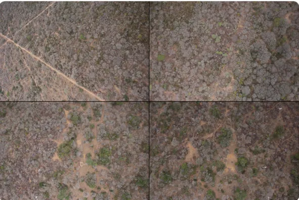
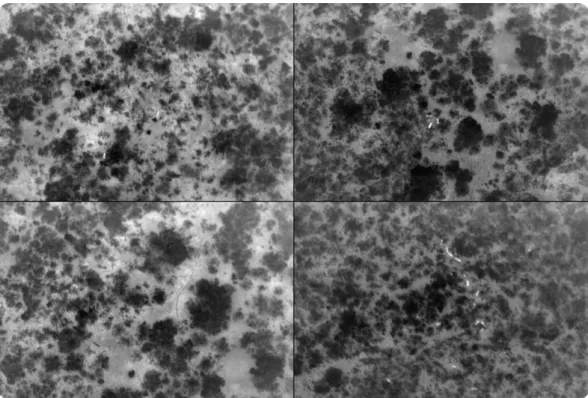
The dataset consists of 890 images (samples), including 121 images that contain at least one elephant (positive samples), 769 images that contain an animal that is not an elephant (other samples) or images that do not contain any animals at all (negative samples). Each sample con-sists of a 20MP RGB image with a resolution of 3, 600×5, 400 (Figure 1.3), an IR image with a resolution of 480×640 (Figure 1.4), the time of capture, the GPS coordinates of the aeroplane, and two altitude readings, one from the RGB camera and one from a dedicated laser altimeter.

The capture flight path can be seen in Figure 1.5. The erratic and looped path would never be used in a live capture mission, but since the main focus was to capture as many examples of elephants as possible, the pilot was instructed to do multiple flyovers when an elephant was spot-ted. One of the biggest challenges we face with this thesis is the relatively small dataset we have to work with, and even at this point we are using a form of data augmentation by capturing the same elephant groups at different passes. We can safely assume that the samples vary enough between captures that very little bias is introduced into the dataset at this point, since the ele-phants most likely moved, along with the angle and altitude of capture that would be different. The capture time of the dataset is constrained by the ambient temperature, since the difference between the ambient temperature and an elephant’s core temperature needs to be at least 4◦C

for the elephant to appear on the captured thermal image. This poses an interesting challenge, since the only time to capture images would be in the early morning while the ground is still cool, but there is enough light to capture the elephants. Over the two hour flight, the sun will gradually heat up the ground, also decreasing the visibility of the elephants in our thermal images towards the end of the capture session.

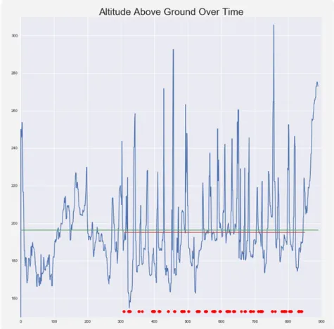
The colour changes in the flight path (Figure 1.5) indicate the change in altitude as the im-ages were captured. Using the dedicated altimeter, we can plot the altitude above ground for

(11)

CHAPTER 1. INTRODUCTION 5

Figure 1.3: Randomly sampled RGB images from the dataset. Most of the landscape is covered with green and grey foliage, with patches of brown soil occasionally breaking through.

each capture over the duration of the flight, as seen in Figure 1.6. The first 300 images in the dataset represent the long tail starting in the lower left corner of Figure 1.5. Once a group of ele-phants is spotted, the pilot starts looping over the group. Each positive sample is represented by a red marker on Figure 1.6. We notice the average altitude of the entire flight (represented by the green bar) is almost the same as the average positive capture altitude (represented by the red bar). The high variance in the altitude over the flight duration and between captures adds an interesting element to our problem. With the altitude fluctuating between 150m and 300m, the size of the elephants in the image also fluctuates significantly. Under ideal conditions we would like to keep the altitude constant, allowing us to construct a traditional computer vision based filter constrained on size and shape to extract the elephants from the images. We can see that this approach will not work here, since we need a scale invariant approach to combat the high variance in altitude and target size.

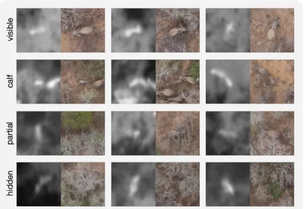
After capture and conversion, the dataset was hand annotated. Each elephant across all the infrared images was marked and hand classified as either visible (adult elephant that is fully vis-ible in the corresponding RGB image), calf (a young elephant that is fully visvis-ible in the corre-sponding RGB image), partial (an adult elephant that is partially visible, and partially obscured from view in the corresponding RGB image), and lastly hidden (an elephant that is not visible at all in the corresponding RGB image). Examples of each can be see in Figure 1.7. The dataset contains 524 visible elephants, 39 calves, 312 partially visible elephants, and 119 fully hidden ele-phants. The true elephant count in the park is around 100 elephants and they move around in three main groups, thus we have increased the dataset size nearly tenfold by using the multiple-flyover technique.

(12)

CHAPTER 1. INTRODUCTION 6

Figure 1.4: Randomly sampled thermal images from the dataset. The darker regions represent the cooler foliage, while the lighter regions represent the hotter soil. All of the images contain elephants, visible as white blobs.

Figure 1.5: Using the GPS data, we plot the flight path used to capture the dataset. Once a group of elephants was spotted, the pilot was instructed to do multiple passes, resulting in the set of tight loops visible in the image.

(13)

CHAPTER 1. INTRODUCTION 7

Figure 1.6: By plotting the sequential altitudes over the duration of the flight, we show the high variance present in the altitude, and as a result the high variance in target size and temperature. The red marks indicate images that contain elephants. We can see the altitude fluctuates between 150m and 300m.

1.3 Our approach

We can see from the RGB images in Figure 1.3 that manually detecting an elephant at these al-titudes is challenging even for a human. With the aid of the thermal images in Figure 1.4, it becomes quite easy to find the elephant shaped blobs and search the corresponding area in the RGB image. This idea forms the foundation of our approach to the problem.

We propose a two phased approach to detecting and classifying elephants from our dataset. Instead of attempting to detect the elephants directly in the RGB image (which is computationally expensive, and comparable to the overwhelming feeling we get by searching for an elephant in the RGB image), we use the IR images to first determine which regions are most likely to contain an elephant before passing those regions onto a classifier.

Figure 1.8 shows where our solution fits into the pipeline. We take the converted and anno-tated data, attempt to reduce the search space of the problem through region proposal before classifying the regions of interest with a trained convolutional neural network. One of the main objectives at each step of the pipeline is to reduce the number of false negatives (without losing an elephant along the way). With this in mind, we will attempt to build a simple and fast region proposal phase with a very high true positive rate, while leaving the true decision power for the classification phase. The goal is to provide a human with a reduced set of options for manual

(14)

CHAPTER 1. INTRODUCTION 8

Figure 1.7: Thermal and visual example pairs of the label categories. Elephants must be clearly visible in both bands to be labelled as visible, the same holds for calves (calf ). Elephants occluded in the visual band are labelled as partial, while elephants only present in the thermal band are labelled as hidden.

Figure 1.8: Data capture, format conversion, and manual verification are necessary steps in the pipeline, but are not in the main scope of this thesis. Our focus is on using the annotated dataset and investigating region proposal strategies that will be used along with a deep learning classifi-cation model to detect the elephants.

verification after the classification phase.

1.4 Similar work

Similar work has been done in the field of animal detection, some using deep learning and aerial drone images to detect marine mammals [8], others using motion detection cameras in the wild along with deep learning [9]. A more modern approach is to use region proposition based

(15)

CHAPTER 1. INTRODUCTION 9

volutional neural networks [10].

The current thesis contributes to this body work through its combination of traditional com-puter vision techniques for region proposal on infrared images and current state-of-the-art deep learning feature extraction methods for classification.

1.5 Thesis outline

The next chapter of this thesis takes a look at the history and theory of computer vision and ma-chine learning that makes our mama-chine vision solution feasible. We then look at ways to process the data to improve our model performance and accuracy, before moving onto the actual im-plementation, experimentation, and results achieved. We draw a conclusion on the outcome, propose potential future work and reflect on the entire process.

In Chapter 2 (Background and theory) we take a theoretical look at core computer vision and machine learning concepts that make the proposed solution possible. We start with classical computer vision and focus on its feature engineering properties. We move onto machine learn-ing, starting with neural networks and transition into the deep learning paradigm, remaining focused on relevant machine vision components. The chapter ends with an overview of software implementations of the discussed theory.

Chapter 3 (Region proposal) focuses on reducing the complexity of the classification task at hand. Using the infrared data, we can reduce the problem space that needs to be searched in the visual band data. We investigate various ways to detect dim targets in the thermal data. Once the targets have been selected, we look at registering the thermal and visual images together. We end the chapter with input that is ready to be used by our deep learning models.

In Chapter 4 (Implementation and results) we look at various ways to create an elephant clas-sification model. We start by training a model from scratch, with randomly initialised weights and experimenting with different model architectures and hyperparameters. We then experiment with fine-tuning an existing model, which is a widely used technique called transfer learning. After putting everything together, we evaluate the system performance of the different models.

Chapter 5 (Conclusion) ends off the thesis by presenting conclusions, proposing possible ex-tensions to the work and reflecting on the process.

(16)

2

|

Background and theory

“Do Androids Dream Of Electric Sheep?”

- Philip K. Dick In this chapter we explore how we quantify vision and give a computer the ability to understand images, in a sense allowing a machine to see. We briefly give an overview of computer vision and why it is such an important field in today’s world. We then move onto machine learning, specifically looking at neural networks and how their modern application as deep neural net-works has disrupted multiple fields, including computer vision. From a theoretical viewpoint we move onto an overview of the practical aspects associated with deep learning, from the most popular libraries to the hardware choices that play a role in the training process.

2.1 Giving a machine vision

Vision is arguably considered the most important sense that we possess. A significant portion of the brain is involved in processing and reacting to visual information [11]. In the pursuit of optimisation and innovation, we would ideally like to allow a machine to also take advantage of all the visual information available in the world.

As intuitive as seeing is for a human, the same does not apply to a machine. For a machine to gain access to visual information, we need to give it a window into the world. This window would be obtained from some form of sensor that converts the analogue visual band into a digital format that it can work with. This format is typically one or more digital images in either colour or greyscale.

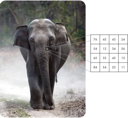
A digital image is represented as a grid of values called pixels. For a colour image the grid is a 3-dimensional matrix with a width, height, and depth (also called channels). The width and height correspond to the sensor that was used to capture the image, and the resolution of the sensor is usually specified in megapixels (MP). The depth of the grid depends on the colour space being used to represent the image, with red-green-blue (RGB) widely used in applications. Each pixel is a quantised representation of the analog light signal that was absorbed by the sensor at that point. Typical pixel fidelity would be 8-bits, resulting in three values ranging between 0 and 255, one for each colour channel. Sensors with higher bit rates allow for more accurate colour representation, but at the cost of higher storage requirements. The representation of visual information as a grid of pixels is illustrated in Figure 2.1.

Assuming a standard digital image with dimensions 64_×64_×3 at 8-bit resolution, we will have 12,288 values that represent the image. From this representation, we would like the computer to understand what is happening in the image. This is an enormous task that has been a topic of research for many years.

The naive approach would be to consider how a human makes sense of visual information and manually model the behaviour. If we take an image of an elephant looking to the right, we would identify the parts that make up the whole. We would look at the distinct features that

10

(17)

CHAPTER 2. BACKGROUND AND THEORY 11

Figure 2.1: Example of the pixels that make up a digital image, visualised is a single channel of values that make up the highlighted image patch.

make up an elephant. Considering the core features of an elephant, we might list ear shape, eye form and presence of tusks as the most important identifiers. Using this information, we would attempt to describe the shape of an ear in terms of pixels and how they relate to each other. It would take many hours and multiple iterations, but we would end up with a system that could identify our elephant image as an elephant. Given a second image of another elephant that is looking slightly up, out system would no doubt fail to identify the image as an elephant. This is an example of overfitting our model to our data, resulting in a system that cannot generalise to the seemingly infinite variations of images that contain an elephant.

We just attempted to manually encode the characteristics of an elephant, a process known as feature engineering. Historically this has been the best known way to approach the problem, resulting in hours spent building models that have value in very narrow problem domains. Even for a very specific problem such as identifying an elephant in an image, we face viewpoint varia-tions, scale variavaria-tions, deformation, occlusion, illumination condivaria-tions, background clutter, and inter-class variations [12], as illustrated in Figure 2.2 through the use of cats.

For a system to be useful, it should be able to handle these and many more variations. Build-ing such a system by manually describBuild-ing every imaginable situation would be infeasible. Thus we need to rethink our approach.

A human child that sees a cat for the first time would be able to associate all of the above variations as still being a cat, without explicitly having seen a cat in each of those situations. This leads us to our second approach; what if there was a way for a machine to learn what a cat is, without explicitly defining its features. This approach can be called feature extraction, and it

(18)

CHAPTER 2. BACKGROUND AND THEORY 12

Figure 2.2: Images from a single image class can contain many variations which make it difficult to describe the class by hand. We see cats and kittens in various positions, behind objects and under different illumination conditions.

requires that we build a model that learns a fundamental representation of visual information. To do this, we require a significant amount of data. This is one of the reasons why this approach has only become feasible during recent years, with the growth of the internet and availability of millions of images.

Now that we have established how a computer represents the visual world in the form of images and come to the conclusion that it is really difficult to explicitly explain to a computer what is going on in an image, we can investigate ways to make a computer learn meaning and representation on its own.

2.2 Let it learn

Learning is so intuitive that we rarely stop to think what it really means to learn. For a computer we would define it as an algorithm that learns from a set of data [13]. A formal definition was given by Mitchell [14]: “A computer program is said to learn from experienceE with respect to some class of tasksT and performance measureP, if its performance at tasks inT, as measured byP, improves with experienceE”.

To continue our example, our current task is to identify elephants in a set of images. The experience consists of all the different images in the set, and the performance can be calculated as how accurately the model identifies the elephant images as elephants and the non-elephant

(19)

CHAPTER 2. BACKGROUND AND THEORY 13

images as not elephants.

There are a lot of different tasks in machine learning. The most relevant task to this thesis, and the only one we will focus on, is the task of classification. In a classification task we ask the algo-rithm to assign a probability that a specific image belongs to one of a finite set of categories. In our example we have a binary classification task where the image is either designated as elephant or not elephant.

Goodfellow et al. [13] define a simple recipe for a machine learning algorithm as the combi-nation of a dataset, a cost function, an optimisation process, and a model. We can break up each of these components to gain an understanding of how they make up the learning process. The following is a high level overview of the learning process, and the sections that follow will go into more detail.

Starting with the dataset, we first need to make the distinction between supervised and un-supervised learning. With the former our experience is a set of images with manually assigned labels. That is to say each image in the dataset has its relevant category assigned to it before the learning process starts. This allows us to calculate the performance and learn from the ex-perience by comparing the predicted result (the task) with the known label of the image. With unsupervised learning we are given an unlabelled dataset. This means that we have no class information of the images before the learning process starts and thus we do not have a simple way to measure the performance of the classification task. The scope of this thesis is mainly on supervised learning and we will not go into further details regarding unsupervised learning.

Given a labelled dataset that consists of elephant and not-elephant images, our goal is to end up with a model that can accurately classify the images into the correct categories. We start off with the assumption that a set of rules exist that will satisfy this goal. This is a realistic tion, simply taking into account that is seems to be a trivial task for a human. With this assump-tion in mind, we attempt to mathematically model a similar system in code. In its simplest form, this is represented as a mathematical function f(x)₌y, wherexis the input to our model,yis the class prediction andf is our model. Our modelf can take many forms, and one of the biggest challenges in machine learning is to find the most appropriate model for a given problem. For the moment accept thatf is chosen appropriately for our elephant classification challenge. For our given model, we want to find the ideal parameters for our function that will correctly classify our dataset.

The optimisation process is used to iteratively “learn” the ideal parameters. As mentioned earlier, our system learns from an experience when the performance on a task increases. Thus we need a way to measure the performance of our model (our task) on the dataset (our experience). We can define a cost function that will act as the performance measure. This cost function is usually defined as a distance metric that can quantify how well a model can predict the correct classes for the images in the dataset.

With our recipe in hand, we move to a class of models that hold the most promise for image classification: the neural network.

2.3 The foundation of neural networks

The universal approximation theorem states that a neural network with a single hidden layer of finite neurons and any continuous sigmoidal nonlinearity can approximate any continuous func-tion ofnreal variables [15]. This means that structured high-dimensional data such as languages, sounds, and images can be approximated and represented by a neural network model.

To understand neural networks, we must first discuss what inspired their design and what potential they might hold. The idea of artificial intelligence has been with humanity since ancient times, such as the golem made from mud, in search of intelligence and the divine [16]. In the spirit of biomimicry, we look to our own minds in search of a solution to intelligence. The idea of modelling the human brain was first attempted in modern times in 1943 by McCulloch and Pitts

(20)

CHAPTER 2. BACKGROUND AND THEORY 14

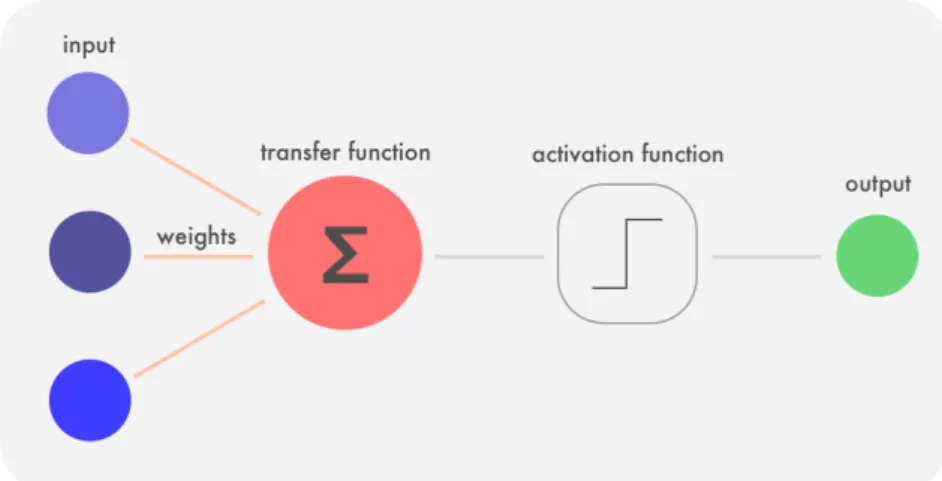
Figure 2.3: A model of a neuron used in a perceptron. The blue input values are combined with the connection weights in the red transfer function, and the real valued output from the transfer function is either activated (1) or not (0) in the activation function using a set threshold value. The activation value is passed along in the network as the green output value.

[17], when they modelled a simple neural network using electrical circuits. This led Rosenblatt [18] to create a mathematical model (a perceptron) that attempts to explain how the neurons in our brain works. A perceptron consists of multiple neurons (Figure 2.3), each taking a set of binary inputs (either model input or from other neurons), multiplying these input values by continuous learned weights, and finally thresholding the sum of these weighted values either to activate the neuron (with a value of 1), or to keep it dormant (with a value of 0). It can be shown that a perceptron can model basic boolean gates, which seems to imply that it is capable of logical reasoning and ultimately artificial intelligence. With a simple model of the brain at hand, a natural question arises: how do we get our artificial brain to learn? Backpropagation was proposed in the early 1960s and has been of interest in academia since, but it was in 1989 that LeCun et al. [19] demonstrated the real world feasibility of backpropagation by training a neural network to recognize handwritten digits. With the continuous advances in technology along with popular acceptance of backpropagation, we rapidly advanced towards more complex models and techniques, soon arriving at what we today know as deep learning.

Before we move to deep learning concepts, we take a brief look at the most important neural network components that we will be using to solve our classification problem.

The feedforward neural network (also called a multilayer perceptron) is a fundamental deep learning model, taking an inputx, passing it through the model f to get outputy. This is done in a single pass without any feedback back into the function, earning it the feedforward name [13]. Feedforward neural networks are widely used in machine learning and are a foundation component of deep learning and convolutional neural networks.

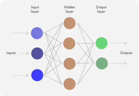
The feedforward neural network (Figure 2.4) consists of one or many hidden layers that con-tain multiple neurons. Each neuron concon-tains a weight vector that is initialised with random val-ues [20], but is tuned to the classification problem at hand through training. Every neuron has an activation function that determines its output value, given all input values and its internal weight vector. Popular choices for the activation function include the sigmoidal nonlinearity [15] and the rectified linear unit (ReLU) [21]. To train these weights we used an optimisation process such as stochastic gradient descent (SGD) [22] along with backpropagation [21] to iteratively minimise our cost function. During training the cost function measures the error between the classified output label and the actual output label, and the cross entropy loss [13] is a popular choice.

Training a feedforward neural network is a supervised learning task, requiring a labelled train-ing set to optimise against, as well as a validation set to estimate the model performance and to

(21)

CHAPTER 2. BACKGROUND AND THEORY 15

Figure 2.4: Simple graph representation of a feedforward neural network. The blue input nodes in the input layer are connected to all of the brown hidden nodes in the hidden layer, while all the brown hidden nodes are in turn connected to all of the green output nodes in the output layer. The information flows from one layer to the next, never flowing back into a previous layer.

guide hyperparameter selection during training [13]. To prevent the model from overfitting we use techniques such asL2regularisation [13].

With our foundation set, we dive into deep learning and more specifically the convolutional neural network models that we will be using to train our classifier.

2.4 Deep learning and convolutional neural networks

Deep learning is a direct extension of neural networks, since the concept of a deep neural net-work comes from a neural netnet-work with multiple hidden layers. Even the arguably shallow two layered neural network could be considered deep. Deep learning is not a new concept, but has been limited by input data volume and computation power, both of which are no longer a re-strictive issue. The recent growth in deep learning interest started with the seminal paper by Krizhevsky et al. [21] in 2012. They showed how the hierarchical structure of a deep neural net-work could be used to learn feature representations from visual images. The model performance was significantly better than any of the previous feature engineered methods employed in earlier years. An in-depth review of deep learning is given by LeCun et al. [23]. This was also the starting point for us when we started researching the problem of image classification using deep learning. Convolutional neural networks introduce the convolutional layer into our existing feedforward neural network toolbox, and allows us to work with visual data and ultimately train our elephant classifier.

We will look at the three most important layers in a traditional convolutional neural network used for classification: the convolutional layer, the pooling layer, and the fully connected layer.

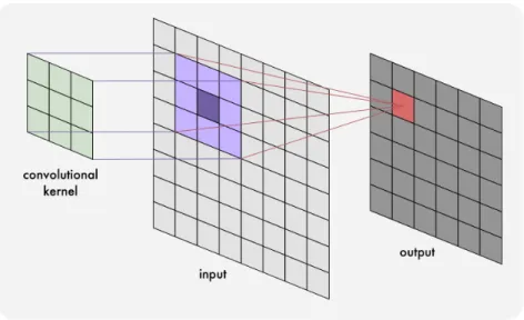
Convolution is a simple mathematical operation that is used to combine (or convolve) infor-mation. In computer vision we use convolution in two dimensions by moving a small convolu-tion kernel over the input image to produce a new output image, as shown in Figure 2.5. The convolutional layer consists of multiple convolutional kernels (also known as filters), which are

(22)

CHAPTER 2. BACKGROUND AND THEORY 16

Figure 2.5: An example of how an 8×8 input image is convolved into a 6×6 output image when a 3×3 convolutional kernel is applied using a stride length of 1 across the entire input image.

the layer weights that need to be tuned during training to extract and activate on relevant features in the input image. Each convolutional layer in a network can flow into another convolutional layer, which allows the network to learn hierarchical features [13]. Starting with simple image parts such as edges and gradients in the first layers, we end up with complex object parts such as elephant body shapes. An example of a single filter applied to our elephant images is shown in Figure 2.6. It seems to successfully extract the shape information of an elephant (amongst other shapes). The size of a convolutional kernel is called the receptive field. By learning filter weights that move across an input image we are locally connecting our filter weights to the input. This reduces the number of parameters we need to train (called parameter sharing), and allows us to train features that are translation invariant. We specify the depth of a convolutional layer to determine the number of unique features we would like the layer to learn, and this depth is a hy-perparameter of the layer. Another hyhy-perparameter is the stride length, which specifies by how many pixels the filter will move between every convolution operation. A larger stride size will result in a smaller output (as well as more information loss between layers). Since a convolution operation results in information reduction we typically end up with a smaller output compared to our input. By zero-padding the output we can control its size as it moves through our network. Each convolutional filter output is called a feature map. All feature maps created by a convolu-tional layer pass through an activation function to produce an activation map [12], sometimes called the detector stage [13]. This is the same nonlinear activation function discussed earlier, with ReLU being a popular option due to its positive impact on training times. ReLU can be im-plemented as a simple threshold operation, compared to the more computationally expensive activations, such as the sigmoidal function.

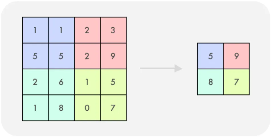
The pooling layer (also called the subsampling layer) is used to reduce the spatial size be-tween different layers [24]. There are different pooling strategies such as average pooling,L2

-norm pooling, and the most popular max pooling (shown in Figure 2.7). All of them result in information reduction, reducing the number of network parameters and computations required by subsequent layers. The need for pooling layers is debated, since they remove a lot of informa-tion from the network. It can be considered beneficial, since it acts as a form of regularisainforma-tion to reduce model overfitting as well as makes our network invariant to small translations in the input [13]. Due to the increase in feature maps created as we go deeper in our network we need to pool between convolutional layers to prevent parameter combinatorial explosion.

(23)

CHAPTER 2. BACKGROUND AND THEORY 17

Figure 2.6: We selected a single convolution filter that looked promising from one of the first neural networks that we trained. We convolved a few of the training images with this filter and obtained this result. It is interesting to note how a single 3_×3 filter can extract so much shape information from the images. This result motivated us to continue investigating deep convolu-tional neural networks as a solution.

(24)

CHAPTER 2. BACKGROUND AND THEORY 18

Figure 2.7: We illustrate a 2×2 max pooling operation with a stride length of 2 pixels. Similar to the convolution filter, we move the pooling window across the input and use the maximum value found inside the pooling window as the output. By doing this we introduce translation invariance into the model, as well as reduce the number of parameters in the network by reducing the activation map sizes being used as input by subsequent convolutional layers.

A fully connected layer (also known as a dense layer) is the same hidden layer discussed in the previous section under feedforward neural networks. Compared to the local connectivity of the convolutional layer, a fully connected layer connects every one of its neurons with every input from the previous layer. Each neuron has a weight vector that needs to be trained and an activa-tion funcactiva-tion that determines its state after multiplying the neuron input with its weights. Given the fully connected nature of the layer, we see a growth in parameters in the network (since each neuron in the layer needs to be connected with every activation map). A fully connected layer is usually used as the final layer in a convolutional neural network, and their activations corre-spond to the higher level features detected in the activation map from the previous layer. These activations are connected to a softmax classifier, which applies logistic regression to the activa-tions to calculate class probabilities for the input image. These class probabilities correspond to normalised real values that represent the confidence of the input belonging to the given class [25].

Given the three layers just discussed, we can build the simplest architecture that takes an input image, passes it through a convolutional layer that creates multiple activation maps, re-duces the map size though pooling, and passes the activations through a fully connected layer that classifies the input into classes using a softmax classifier (as seen in Figure 2.8).

We can use these building blocks to create increasingly complex and deep networks. One of the earliest successful applications of a convolutional neural network was the LeNet network [26] in 1998 that consisted of seven layers, a small extension to the basic model shown in Fig-ure 2.8 by adding a second convolution and pooling pair. In 2012 Krizhevsky et al. created the eight layer deep AlexNet [21], winning the ImageNet ILSVRC 2012 challenge and starting the age of deep learning. AlexNet was similar to LeNet, except with more parameters, a slightly deeper architecture, and stacked convolutional layers. VGGNet [27] was the runner-up in the ImageNet ILSVRC 2014 competition and showed that increasing the depth of the net had a positive im-pact on the model performance. Two variations were trained, namely VGG16 with 16 layers and VGG19 with 19 layers. All of these models are visualised in Figure 2.9. In 2015 Google created InceptionV3 [28], which was an improvement on the original GoogleLeNet [29] that won the Im-ageNet ILSVRC challenge in 2014 with a 22 layer deep architecture. The GoogleLeNet and Incep-tion architectures strayed from the accepted format of stacking layers sequentially by splitting and joining (concatenating) the network at various depths, as seen in Figure 2.10.

(25)

CHAPTER 2. BACKGROUND AND THEORY 19

Figure 2.8: The simplest convolutional neural network architecture we can build that includes our foundation convolution, pooling, and fully connected (or dense) layers. The convolution layer includes an activation function. The output layer represents the softmax classifier that predicts the class labels using the activations in the previous dense layer.

Figure 2.9: An illustration of popular architectures that have influenced the direction of deep learning research. LeNet was the first to show the value of convolutional neural networks in a image classification task. By winning the ImageNet ILSVRC 2012 challenge, AlexNet showed the potential that deep learning holds. VGG19 continued the tradition of building deeper and more complex models, showing that the depth of an architecture had a notable impact on per-formance.

(26)

CHAPTER 2. BACKGROUND AND THEORY 20

Figure 2.10: InceptionV3 schematic diagram showing the split and join operations throughout the network architecture. Image from [30].

Before an architecture can be used it needs to be trained. Once a network is built all its weights and biased need to be given initial values. There are multiple strategies that include setting all weights to zero (all neurons initially calculate the same result, which makes this a bad choice), selecting random values (which will allow the neurons to calculate unique results from the start), uniform distribution initialisation (a common heuristic which uniformly generates and distributes the weights), along with more advanced methods such as Xavier initialisation [31] and ReLU initialisation [32]. These strategies of weight initialisation are called training from scratch. Another strategy is to use weights from pre-trained networks, such as AlexNet or InceptionV3. This is called transfer learning and usually provides the fastest route to a well performing model [33]. Transfer learning can be used in various ways, the simplest being to train a classifier on the different layer activations generated by predicting the values of a training set. The existing weights can also be modified, or fine-tuned, to another problem domain.

Both training from scratch and fine-tuning require a training strategy. This strategy iteratively attempts to improve the weights on the model in order to minimise a set cost function [13]. This cost function is the error between the predicted label and the actual value, and a common choice is to use the softmax prediction values and to calculate the cross entropy loss [13] to measure the intensity of the prediction, in other words how correct or incorrect the prediction was. The strat-egy consists of one or more epochs, where an epoch is completed when the model has seen all of the training images once [13]. The model sees the training images in batches, which limits the number of images seen per iteration, thus an epoch consists of multiple batch iterations before it completes. The rate at which the model adjusts the weights is known as the learning rate [13], and is used by the optimisation strategy to find the best direction to move the weight values in. Popu-lar optimisation strategies rely on gradient descent, including stochastic gradient descent (SGD) [22], AdaGrad [34], and Nadam [35]. Some of these methods rely on momentum [36], which al-lows the learning rate to increase (and the search range in the search space) if the direction of change remains consistent between iterations. A popular momentum strategy is Nesterov mo-mentum [36] (employed by Nadam). Another option is to vary the learning rate over the training period, allowing it to decay over time (either linearly, quadratically, or exponentially), as used by AdaGrad [37].

To prevent overfitting to the training data (and hopefully generalise to the problem at hand), there are a few common regularisation strategies that we can employ. By adding dropout [38] during training we ignore a neuron (and its connections) with a set probabilityp, removing it from consideration during some iterations and preventing fixed activation paths from forming around certain training images (which is overfitting). Another way is to generate pseudo-unique images from our training data, a strategy called data augmentation [21], and allows relatively

(27)

CHAPTER 2. BACKGROUND AND THEORY 21

small datasets to be used as input to deep learning models. Typical augmentation types include translation (horizontal and vertical), rotation, scaling, shearing and flipping. Batch normalisa-tion normalises each training batch, and also allows for higher learning rates to be used [39].

One would think the next step in the process is to grab your favourite editor and start writing clear, concise and working code. This might have been the feeling at the start of the thesis, but there are some practicalities to consider.

2.5 Practical considerations

In the early days of deep learning it was difficult to find clear documentation and robust im-plementations of the algorithms we just discussed, since most of the available resources came from research oriented sources that were still figuring out the best way to implement them. As the popularity of deep learning grew through commercial application, more funding was allo-cated to both academic and commercial research and development. This, along with the rapid improvement in hardware performance and efforts by Nvidia to support the growing interest in deep learning resulted in stable libraries, powerful hardware, and cloud infrastructure that took advantage of both to offer powerful solutions to academia and industry alike. We take a look at some of the libraries that we used, along with the improvements between the years 2015 and 2017.

2.5.1 Libraries

Through the power of open source communities it is possible to create and support massive li-braries that contain all of the core algorithms and processes of deep learning. Without these libraries we would not have the advancements in industry that we see today, since it would just be the large corporations that would have access the resources and manpower to create these systems. Luckily the mindset has shifted to an open source mentality, allowing anyone access to the same tools and resources used by these corporations. There is no need to reinvent the wheel, only to adapt it to the specific needs of your problem.

In 2015 we used two popular deep learning libraries at the time, Theano [40] and Caffe [41]. Theano is not specifically aimed at deep learning, but rather a numerical computation library written in Python by LISA labs at the Université de Montréal. It was designed to evaluate math-ematical expressions involving multi-dimensional arrays in an efficient manner [40]. Its wide use within deep learning research has made it synonymous with more specialised deep learning frameworks. Give the more abstract nature of Theano, we used the Python libraries Lasagna [42] and NoLearn [43] to build and train our models. These libraries implemented the core elements (such as backpropagation) and allowed us to easily write the training and evaluation routines we required. Caffe was designed with deep learning in mind, by Berkeley AI Research (BAIR) and written in C++ (along with a Python interface that was used in this thesis). We used Caffe to load pretrained model weights and attempt our transfer learning experiments.

In the years since the improvements in theory, best practises and community support have led to new and more powerful libraries. The most popular of these is TensorFlow by Google. Ten-sorFlow is similar to Theano, in that it is also a numerical computation library designed around nodes and dataflow graphs. “Nodes in the graph represent mathematical operations, while edges represent the multidimensional data arrays (tensors) communicated between them” [44]. Ten-sorFlow is used internally by Google for research as well as systems running in production, and the availability of such a powerful framework as an open source project is truly amazing. Similar to Lasagna and NoLearn, we now have the Keras library [45] that builds on top of both TensorFlow and Theano. Keras is a simple and powerful high-level neural network API written in Python. It allows fast prototyping and abstracts away the technicalities that are not related to the problem one is trying to solve. We used Keras to define, train, and evaluate all our 2017 models.

(28)

CHAPTER 2. BACKGROUND AND THEORY 22

2.5.2 Hardware

Other than the availability of data, computational performance has been a major factor that led to the popularity and success of deep learning. With the advances in graphical processor unit (GPU) architecture in recent years we have seen model training times go from weeks down to hours. Naturally this has allowed us to attempt larger challenges that still take weeks to train, such as Google’s AlphaGO [46] which was initially trained on 176 GPUs and later on proprietary tensor processing units (TPUs) developed by Google.

In 2015 we trained our models on a desktop computer with the best GPU on the market, the Nvidia Titan Z. This GPU has 12GB of memory and 5,760 CUDA cores. Most of our models trained for about 48 hours. There were few alternatives available, with the Amazon AWS cloud platform being the best option. It was a costly option without much support, and the available GPU instances were not as powerful as our Titan Z GPU.

In 2017 the landscape has changed and the cloud options provide the best value for most research and commercial applications. The GPU instances have grown and the economies of scale have allowed the prices to reasonable and fair levels. We trained all our models using the Amazon p2.xlarge instance, with an Nvidia K80 GPU (24GB RAM, 4,992 CUDA cores). On paper it might seem that the Titan Z is more powerful, but using the cloud allowed us to run nine instances simultaneously, allowing us to do hyperparameter optimisation on a 180 model batch run.

2.5.3 Cloud, platforms, MLaaS

As of writing this thesis there are are numerous cloud based options available to do machine learning and deep learning work on. The most popular options are Amazon AWS, Google Cloud, and Microsoft Azure. While they started by only providing the infrastructure as a service (IaaS), they now provide tools and services that cover the entire machine learning pipeline, offering ma-chine learning as a service (MLaaS). This includes Azure Internet of Things (IoT) by Microsoft, Alexa Machine Learning by Amazon, and Cloud Vision by Google. The cost of using these ser-vices is usually determined on a pay-per-use basis, such as the Amazon p2.xlarge instance that costs $0.9 per hour of usage.

A new form of machine learning service that has emerged is one that offers a full commercial pipeline solution from data collection all the way to deployment and versioning. One of the lead-ers in this market is Valohai [47], a company situated in Turku, Finland. One of their goals is to allow academic research to be easily reproducible and verifiable using their platform. The team at Valohai has given me access to their beta platform, and all of the 2017 experiments were run on this.

Valohai relies on the Amazon GPU infrastructure, but adds value by relying on version control to setup experiments, by automatically generating graphs from training metadata, and automat-ically caching and storing model training data and results. Some of the features are illustrated in Figure 2.11. An experiment is uploaded to a GIT repository along with a Valohai configuration file that specifies the experiment parameters, such as dataset location and hyperparameters. We can perform hyperparameter optimisation as a task by setting possible values for these hyperpa-rameters, which will create an execution from each combination of hyperparameter options. An active execution will log and graph all output specified by us in the experiment. We can run ex-periments in parallel, setting how many instances we would like to use for a specific task. We used nine active p2.xlarge instances on all our experiments. All logs and output files are archived in the cloud for easy evaluation. The value that Valohai adds are things that are (or should be) done during research and experimentation. It is just another example of how our development and research workflows can be optimised and automated for more efficient work and record keeping. Continuing on, we start implementing our solution in Chapter 3 by looking at the infrared images and how they can be used to propose regions of interest for our deep learning classifier in Chapter 4.

(29)

CHAPTER 2. BACKGROUND AND THEORY 23

Figure 2.11: Screenshots of the Valohai platform that was used to run the 2017 experiments. Tasks were used to run hyperparameter optimisation batches, with each model execution having its own setup, log, and metadata views.

(30)

3

|

Region proposal

“Complexity is your enemy. Any fool can make something complicated. It is hard to keep things simple.”

- Richard Branson The purpose of region proposal is to reduce the number of queries that we need to submit to our classifier in Chapter 4. By ranking areas by likelihood, we can eliminate a lot of work and save our most important resource, time. The classification phase is the most resource intensive, so the more pre-work we can do using cheap and fast methods, the better. Thus this chapter will focus on using traditional image processing techniques on the infrared data to propose regions of interest that will ultimately be classified by our deep learning models.

Our goal is to build a cheap and fast region proposal algorithm that attempts to minimise false negatives, while keeping the number of non-elephant regions detected as elephant regions as low as possible. This means that we do not want to lose any elephants during this phase, even at the cost of a large number of false positive detections.

3.1 Infrared blob detection

Infrared (IR) imagery is used in many domains. Most of the early work focused on military appli-cation for offence and defence, while more recent work has focused on more constructive uses such as nature conservation. An example of one of our IR images can be seen in Figure 3.1. A long range infrared sensor was used to capture the image, and each pixel value is actually a real val-ued temperature measurement. The image was created by scaling all of the temperature values between 0 and 255, with the hottest measurement at 255 and the coldest at 0. All of the images were captured in the early morning, just after dawn when the earth is still cool before the African sun heats it up.

One of the key requirements of IR to be useful is that the target object has an internal tem-perature that is different from the ambient temtem-perature by at least 4◦C. If this requirement is not met, the sensor will not be able to distinguish between the object and the background around it. This allows for a very small window when the data can be captured, since multiple factors such as the current and previous day’s weather could drastically influence the quality and usability of the captured data.

Since our data is captured every four seconds from a moving aircraft, we have a single snap-shot to work with, and fall into the single image-based detection group. An example of detecting pedestrians in infrared images [48] allows a stationary camera to capture multiple images over time, for sequential image-based detection methods to be applied. These methods take advan-tage of the constant background data between sequential images, thus allowing for background removal and ultimately isolating the moving targets in the image. A defence application of this is the sea-based searching, detection and tracking of a moving missile through its heat signature against a static background or cluttered background [49].

24

(31)

CHAPTER 3. REGION PROPOSAL 25

Figure 3.1: Infrared image showing four targets. The colder trees are visible as darker patches, in contrast to the warmer ground which is a lighter grey.

A similarity shared between all of these applications is the need to isolate and detect a dim target against a complex and cluttered background. In search of a solution, we first look at blob detection.

A blob is a mostly homogeneous region in an image that differs in shape and intensity from its surrounding area. Blob detection has traditionally been used to propose regions of interest, but has fallen out of favour with the advancements in computer vision and machine learning.

We are interested in this technique, because its simplicity is exactly what we need for our com-putationally cheap and fast region proposal algorithm. We will rely on some feature engineering to build our solution, making assumptions about the shape and form of our target. These are rea-sonable assumptions to make, since we know the general shape of an elephant in the IR images is approximately oval with a varying degree of rotation.

Some of the challenges we face are uneven exposure, orientation changes, large altitude fluc-tuations, and occlusion. We investigated some of the most popular techniques using the OpenCV [50] Python library. These included the Laplacian of Gaussian (LoG) and Lindeberg’s watershed-based grey-level blob detection algorithm [51]. The most successful of these was the top-hat transformation.

Mathematical morphology theory naturally applies to digital image processing, relying on the assumption that an image consists of structures that can be explained by set theory [52]. It is mainly used with binary (black and white) images, but is easily extended to greyscale images. We use these morphological operations to enhance and ultimately detect dim infrared targets embedded in a cluttered and heterogeneous background. We chose the top-hat transform for its ability to increase the contrast between our targets and the background, given the prior knowl-edge about the target shape and size. As Glasbey [52] explains, “It does this by extracting small or

(32)

CHAPTER 3. REGION PROPOSAL 26

narrow, bright or dark features in an image. It is useful when variations in the background mean that this cannot be achieved by a simple threshold”.

To understand how the top-hat transformation works, we must first understand the funda-mental morphological operation that is erosion. To erode an image, we need to define a structur-ing elementS. We define the shape, size, and the reference point ofS, which is typically a basic shape such as a square or ellipse. The reference point is a chosen pixel position that will be used by the different morphological operations. We illustrate these concepts in Figure 3.2, with the original imageAin(a)showing the foreground as blue and the background as grey. The structur-ing elementSin(b)is shown as a simple 3_×3 square with a reference point in the centre of the structure. Intuitively we can define erosion as removing (or eroding) away pixels from the edges of our foreground image. We define the erosion ofAbySas

A_ªS₌{(i,j) :S(i,j)⊂A}. (3.1)

By placing our structuring elementSonAat different positions, we look at the reference posi-tion pixel inA. If the reference pixel is foreground, as well as the remaining 8 structuring element pixels, we keep the reference pixel as foreground. On the other hand, if the reference pixel is foreground, but at least one of the remaining 8 structuring element pixels is not, we change the reference pixel to background. If the reference pixel is background, we keep it background. Intu-itively this can be compared to image smoothing, except that the background is never changed into foreground. An example of erosion is shown in Figure 3.2(c).

A complement to erosion is dilation, which has the opposite result onA. We define dilation as

A⊕S=(AcªS)c. (3.2)

Similar to erosion, we place our structuring elementSonAat different positions, again look-ing at the reference position pixel inA. If the reference pixel is background with at least one of the remaining 8 structuring element pixels as foreground, we turn the reference pixel into fore-ground. If the reference pixel is background and all the remaining structuring element pixels are background, we keep it unchanged as background. All foreground reference pixels remain as foreground. The intuitive understanding of the dilation effect onAis that the foreground edges are padded and increased. An example of dilation is shown in Figure 3.2(d).

Using erosion and dilation, we can define two composite operators. We define the opening of

AbySas

ψS(A)=(AªS)⊕S, (3.3)

and the closing ofAbySas

φS(A)=(A_⊕S)ªS. (3.4)

This means that opening ofAbyS is accomplished by first erodingAbyS, followed by a dilation of the resulting eroded image byS, as seen in Figure 3.2(e). Similarly, closingAbySis accomplished by first dilatingAbyS, followed by an erosion of the resulting dilated image byS, as seen in Figure 3.2(f ).

(33)

CHAPTER 3. REGION PROPOSAL 27

Figure 3.2: Illustration of the morphological operations that build up to the top-hat transform, with the foreground shown in blue and the background in grey. The original image is shown in

(a), with the example structuring element shown in(b). Applying the erosion operation on(a)

results in(c), while applying the dilation operation on(a)results in(d). The composite opening and closing operations on(a)result in(e)and(f )respectively. Example from [53].

We can now define the top-hat transform as another composite operation:

A−ψS(A). (3.5)

By subtracting the opened image from the original image, we end up with a peak detector that highlights the brightest areas of our image.

Since we are working with greyscale images, we simply define a binary threshold value that will turn our problem into a binary variant, with everything below the threshold considered back-ground and everything above it considered foreback-ground.

Our region proposal algorithm starts with the top-hat transformation stage. Given our in-put imageA(shown in Figure 3.3), we use an elliptical structuring element of size 6_×6 with a reference point in the centre, and apply the transformation.

The resulting image is shown in Figure 3.4. For the erosion and dilation operations, we used a threshold value of 200. When a pixel is dilated or eroded, the average values of the remaining structuring element pixels was used as the new value. This ensured that we increased the contrast between the foreground and the background, without losing intensity information from the true targets as would be the case with a binary operation.

After the top-hat transformation, we take the resulting imageB and apply a Gaussian blur with a kernel size of 3×3 to smooth out the image. We then apply histogram equalisation to further enhance the contrast of the image. Lastly we threshold and binarise the image, and the resultCfor our example is shown in Figure 3.5.

(34)

CHAPTER 3. REGION PROPOSAL 28

Figure 3.3: An original infrared image showing multiple elephant targets across the image.

Detected regions Detected elephants Accuracy Overdetection Rate

33,608 986 98.80 8202.19%

9,215 961 97.58 2507.71%

5,812 919 93.26 1414.65%

Table 3.1: Performance of three versions of the region proposal algorithm on the 121 images that contain at least one elephant. By experimenting with different hyperparameter values we see how quickly the overdetection rate grows with only a small improvement in detection accuracy.

We detect the contours of the remaining blobs and apply a merging algorithm to join smaller blobs with larger ones. We used the prior knowledge of the elephant size and shape to create realistic blobs, s