Parsimonious Gaussian Process Models for the
Classification of Multivariate Remote Sensing Images
Mathieu Fauvel, Charles Bouveyron, Stephane Girard
To cite this version:
Mathieu Fauvel, Charles Bouveyron, Stephane Girard. Parsimonious Gaussian Process Models
for the Classification of Multivariate Remote Sensing Images. ICASSP 2014 - IEEE
Inter-national Conference on Acoustics, Speech, and Signal Processing, May 2014, Florence, Italy.
IEEE, pp.2913-2916, 2014,
<
10.1109/ICASSP.2014.6854133
>
.
<
hal-01062378
>
HAL Id: hal-01062378
https://hal.archives-ouvertes.fr/hal-01062378
Submitted on 9 Sep 2014
HAL
is a multi-disciplinary open access
archive for the deposit and dissemination of
sci-entific research documents, whether they are
pub-lished or not.
The documents may come from
teaching and research institutions in France or
abroad, or from public or private research centers.
L’archive ouverte pluridisciplinaire
HAL, est
destin´
ee au d´
epˆ
ot et `
a la diffusion de documents
scientifiques de niveau recherche, publi´
es ou non,
´
emanant des ´
etablissements d’enseignement et de
recherche fran¸
cais ou ´
etrangers, des laboratoires
publics ou priv´
es.
PARSIMONIOUS GAUSSIAN PROCESS MODELS FOR THE CLASSIFICATION OF
MULTIVARIATE REMOTE SENSING IMAGES
M. Fauvel
1, C. Bouveyron
2and S. Girard
3 1UMR 1201 DYNAFOR INRA & Institut National Polytechnique de Toulouse
2
Laboratoire MAP5, UMR CNRS 8145, Universit´e Paris Descartes & Sorbonne Paris Cit´e
3
Equipe MISTIS, INRIA Rhˆone-Alpes & LJK
ABSTRACT
A family of parsimonious Gaussian process models is presented. They allow to construct a Gaussian mixture model in a kernel fea-ture space by assuming that the data of each class live in a specific subspace. The proposed models are used to build a kernel Markov random field (pGPMRF), which is applied to classify the pixels of a real multivariate remotely sensed image. In terms of classification accuracy, some of the proposed models perform equivalently to a SVM but they perform better than another kernel Gaussian mixture model previously defined in the literature. ThepGPMRF provides the best classification accuracy thanks to the spatial regularization.
Index Terms— Kernel, remote sensing images, Gaussian pro-cess, parsimony, hyperspectral.
1. INTRODUCTION
In a multivariate remote sensing images, a pixel is represented by a vectorx ∈Rdfor which each component is a measurement corre-sponding to specific wavelengths [1]. The classification of such im-ages requires algorithms that are robust to the numberdof spectral wavelengths and that are able to include additional spatial informa-tion in the classificainforma-tion process [2].
Kernel methods, such as SVM, have shown good abilities in classifying images with a large number of spectral bands [3]. The use of a kernel function that defines a measure of similarity between two samples, here two pixel-vectors, make them robust to the spec-tral dimension. However, including spatial information in the clas-sification process is not easy, and the resulting algorithms usually involve a separate step for the extraction/inclusion of the spatial in-formation [2].
On the contrary, conventional statistical method such as Markov random fields (MRF) model the spatial relationship between adja-cent pixels in a proper way by using a local energy function
U(yi|xi,Ni) =−ln p(xi|yi)
+ρE(Ni) (1)
whereyiis the label,p(xi|yi)the conditional probability of having xigivenyi,Eis an energy term that characterizes the local context of
the pixel,Nirepresents the neighborhood ofxiin the spatial domain
andρis a positive parameter. The statistical modeling in the spec-tral domain usually suffers from the increase of the dimension. With the conventional Gaussian assumption,p(xi|yi=c)∼ N(µc,Σc),
the number of parameters of the model scales with the square of the number of spectral variables, which makes difficult reliable estima-tions.
Several approaches have been proposed to combine MRF and kernel methods. The main problem is to compute properly the con-ditional probability in the MRF energy function. Indeed with kernel
functions, the samplesxare implicitly mapped toφ(x)that live on a feature space. For the commonly used Gaussian kernel function, the dimension of the feature space is infinite, and probability functions cannot be defined. Several strategies were proposed to overcome this difficulty. In [4], it was proposed to use SVM to estimate the con-ditional probabilityp φ(xi)|yiin the MRF energy function.
How-ever, the estimated probability is not a true probability, but a scaled version of the SVM output [5]. In [6], the authors defined theoreti-cally the conditional probability in the kernel feature space, but they assumed that the covariance matrices were common to the differ-ent classes in the feature space. A similar assumption regarding the covariance matrix was done in [7]. Although the performances of the above mentioned method were good, such assumption about the covariance matrix could limit the effectiveness of the methods.
In this paper, a family of parsimonious Gaussian process models is proposed to computep φ(xi)|yi
in eq. (1). These models allow to build from a finite set of training samples, a Gaussian mixture model in the kernel feature space, even in the infinite dimensional case. They assume that the data of each class live in a specific sub-space of the kernel feature sub-space [8].
The remainder of the paper is organized as follows. Section 2 presents the family of parsimonious Gaussian process models. Sec-tion 3 focuses on the experimental results on one real hyperspectral images. Finally, conclusions and perspectives are discussed in Sec-tion 4.
2. CLASSIFICATION WITH PARSIMONIOUS GAUSSIAN PROCESS MODELS
2.1. Gaussian process in the kernel feature space
LetS =(xi, yi) n
i=1be a set of training samples, wherexi ∈J,
J⊂Rd, is a pixel andyi∈ {1, . . . , C}its class, andCthe number
of classes. For short, in the following−lnp φ(xi)|yi
will be referred toΩ(φ(xi), yi).
In this work, the conventional Gaussian kernel function
k(xi,xj) = exp −kxi−xjk 2 Rd 2σ2 ! , σ >0, (2)
is used. Its associated feature space isFand the mapping function isφ :Rd
→ F. From the Mercer theorem, we havek(xi,xj) = hφ(xi), φ(xj)iF and the kernel evaluation can be written as (the
series converges absolutely and uniformly for almost all (xi,xj)) [9]:
k(xi,xj) = dF X
m=1
wheredF = dim(F), {em, m = 1,2, . . .}is the sequence of
positive eigenvalues in decreasing order of the integral operatorTk, (Tkf)(z) =RJk(z,x)f(x)dx, associated tokand{vm :Rd→
R, m = 1,2, . . .}is the sequence of corresponding normalized eigenfunctions. From eq.(3),φcan be defined as
φ:x7→√emvm(x), m= 1,2, . . . (4) For the Gaussian kerneldF = +∞[9]. Therefore the conventional multivariate normal distribution cannot be defined.
To overcome this, let us assume that φ(x), conditionally on
y = c, is a Gaussian process with meanµcand covariance
func-tionΣc. Hence, for allr ≥ 1, random vectors onRr defined by
[φ(x)1, . . . , φ(x)r]are, conditionally ony=c, a multivariate
nor-mal vectors. Therefore, it is possible to write foryi=c
Ω(φ(xi), yi) = r X j=1 " hφ(xi)−µc,qcji2 2λcj +ln(λcj) 2 # +γ (5)
whereλcj is thejth eigenvalue ofΣc in decreasing order,qcj its
associated eigenvector andγa constant term that does not depend onc. If the Gaussian process is not degenerated (i.e.,λcj6= 0,∀j),r
has to be large to get a good approximation of the Gaussian process. Unfortunately, only a part of the above equation can be computed from a finite training sample set:
Ω(φ(xi), yi) = rc X j=1 " hφ(xi)−µc,qcji 2 2λcj +ln(λcj) 2 # | {z } computable quantity + r X j=rc+1 " hφ(xi)−µc,qcji 2 2λcj +ln(λcj) 2 # | {z }
non computable quantity
(6)
whererc= min(nc, r)andncis the number of training samples of
classc.
2.2. Parsimonious Gaussian process
To make the above computational problem tractable, it is proposed to use a parsimonious Gaussian process model in the feature space for each class.
Definition 1 (Parsimonious Gaussian process) A parsimonious Gaussian process is a Gaussian processφ(x)for which,
condition-ally to y=c, the eigen-decomposition of its covariance operatorΣc
is such that
A1. It exists a dimensionr <+∞such thatλcj= 0forj≥r
and for allc= 1, . . . , C.
A2. It exists a dimensionpc<min(r, nc)such thatλcj=λfor
pc< j < rand for allc= 1, . . . , C.
The assumptionA1is motivated by the quick decay of the eigen-values for a Gaussian kernel [10]. Hence, it is possible to findr <
+∞such asλcr ≈0. The assumptionA2expresses that the data
of each class live in a specific subspace of sizepc, the signal
sub-space, of the feature space. The variance in the signal subspace for the classcis modeled by the parametersλc1, . . . , λcpcand the
vari-ance in the noise subspace, common to all the classes, is modeled by
λ. This model is referred to bypGP0.
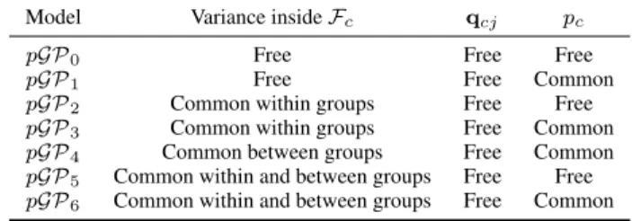
Table 1. List of the sub-models of the parsimonious Gaussian pro-cess model.Fcrefers to the signal subspace of the considered class.
Model Variance insideFc qcj pc
pGP0 Free Free Free
pGP1 Free Free Common pGP2 Common within groups Free Free pGP3 Common within groups Free Common pGP4 Common between groups Free Common pGP5 Common within and between groups Free Free pGP6 Common within and between groups Free Common
From this model, it is possible to derive several sub-models. Ta-ble 1 lists the different models that can be built frompGP0. For the
modelpGP1, it is additionally assumed that the data of each class
share the same intrinsic dimension, i.e.,pc =p, ∀c∈ {1, . . . , C}.
In the modelpGP2, the variance ofFcis assumed to be equal for
all eigenvectors, i.e.,λcj =λc, ∀j ∈ {1, . . . , pc}. For the model
pGP4, it is assumed that the intrinsic dimension is common to
ev-ery class and the variance is common between them, i.e.,λcj =
λc′j, ∀j ∈ {1, . . . , p}andc, c′ ∈ {1, . . . , C}. In term of
par-simony,pGP0 is the least parsimonious model whilepGP8is the
most parsimonious of the proposed models.
In the following, only the modelpGP0 is discussed. Similar
results can be obtained for the other models.
Proposition 1 LettingpM = max(p1, . . . , pC), eq. (5) can be
writ-ten forpGP0as Ω(φ(xi), yi) = pc X j=1 1 λcj − 1 λ hφ(xi)−µc,qcji2 2 + 1 2λkφ(x)−µck 2 + pc X j=1 ln(λcj) 2 + (pM−pc) ln(λ) 2 +γ ′ (7)
whereγ′ is a constant term that does not depend on the indexcof the class.
The computation of eq. (7) is now possible sincepc < nc, ∀c ∈ {1, . . . , C}. In the following, it is shown that the estimation of the parameters and the computation of eq. (7) can be done using only the kernel evaluation, as in standard kernel methods.
2.3. Model inference
Let us define the centered Gaussian kernel function according to classcas: ¯ kc(xi,xj) = k(xi,xj) + 1 n2 c nc X l,l′ =1 yl,y′ l=c k(xl,xl′) − n1 c nc X l=1 yl=c k(xi,xl) +k(xj,xl). (8)
The associated normalized kernel matrixKcof sizenc×ncis
de-fined by (Kc)l,l′ = ¯ kc(xl,xl′) nc . (9)
Ω(φ(xi), yi) = 1 2nc ˆ pc X j=1 1 ˆ λcj 1 ˆ λcj − 1ˆ λ nc X l=1 yl=c βcjlk¯c(xi,xl) 2 + 1 2ˆλ ¯ kc(xi,xi) + ˆ pc X j=1 ln(ˆλcj) 2 + (ˆpM −pˆc) ln(ˆλ) 2 (10)
Table 2. Information classes for theUniversity Areadata set and classification accuracy. SVM refers to the support vectors machine, GMM refers to the Gaussian Mixture Model, KGMM refers to the kernel GMM proposed in [7]and OA refers to overall accuracy.
(a). Information classes Class Samples Asphalt 6631 Meadow 18649 Gravel 2099 Tree 3064 Metal Sheet 1345 Bare Soil 5029 Bitumen 1330 Brick 3682 Shadow 1947 Total 42776 (b). Classification accuracy Method OA pGP0 83.5 pGP1 84.2 pGP2 62.7 pGP3 69.6 pGP4 73.4 pGP5 61.1 pGP6 69.9 SVM 84.5 GMM 77.7 KGMM 80.4 pGPMRF 91.2
Proposition 2 Forc= 1, . . . , Cand the modelpGP0, eq. (7) can
be computed with eq. (10), whereβcjlis thelthcomponent of the
normalized eigenvectorβcjassociated tojthlargest eigenvalueλˆ cj ofKcand ˆ λ=PC 1 c=1ˆπc(rc−pˆc) C X c=1 ˆ π trace(Kc)− ˆ pc X j=1 ˆ λcj (11)
andπˆc=nc/n. See [8] for the proof.
The estimation ofpcis done by looking at the cumulative
vari-ance for the sub-modelspGP0,2,5. In practice,pcis estimated such
as the percentage of the cumulative variance is higher than a given thresholdth: Ppˆc j=1λˆcj Pnc j=1λˆcj > th. (12)
For the other sub-models,pˆis a fixed parameter given by the user.
3. EXPERIMENTAL RESULTS
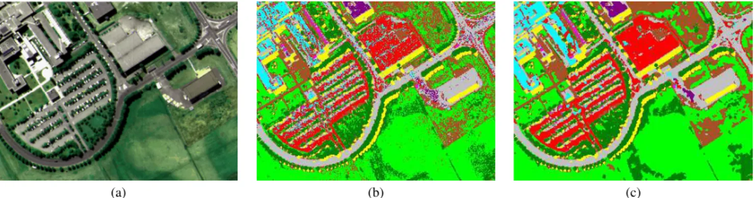
In this section, results obtained on one real data set are presented. The data set is theUniversity Areaof Pavia, Italy, acquired with the ROSIS-03 sensor. The image has 103 spectral bands (d = 103) and is 610×340 pixels, see Figure 1.(a). Nine classes have been de-fined by a photo-interpret for a total of 42776 referenced pixels, see Table 2.(a). 50 pixels for each class have been randomly selected from the samples for the training set, and the remaining set of pix-els has been used for validation. The process has been repeated 50 times, each time a new training set has been generated and the vari-ables have been scaled between -1 and 1. The mean result in terms of overall accuracy (percentage of correctly classified pixels) are re-ported.
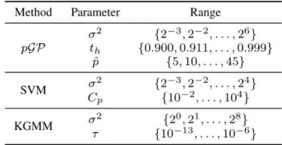
Table 3. Grid search setting for the cross validation.thcorresponds
to the threshold value on the cumulative variance,Cpis the
regular-ization term for the SVM andλr refers to the ridge regularization
term in KGMM.
Method Parameter Range pGP σ2 {2−3,2−2, . . . ,26} th {0.900,0.911, . . . ,0.999} ˆ p {5,10, . . . ,45} SVM σ 2 {2−3,2−2, . . . ,24 } Cp {10−2, . . . ,104} KGMM σ 2 {20,21, . . . ,28} τ {10−13, . . . ,10−6}
To assess the statistical significance of the observed differences in terms of classification accuracy, a Wilcoxon rank-sum test has been applied over the 50 repetitions. It tests if the data from two populations are samples from distribution with equal medians. In the experiments, it is used to test whether the 50 classification ac-curacy are significantly different (not equal medians) or not (equal medians).
Two sets of experiments have been conducted. First, the pro-posed models have been compared to three others models: the support vectors machines (SVM), a conventional Gaussian mixture model (GMM) and a Kernel GMM defined in [7]. These models use only the spectral information from the remote sensing image. Sec-ond, the modelpGP1 has been used to build apGPMRF classifier
that uses both the spatial and the spectral information.
3.1. Comparison with others spectral classifier
In this section, the proposed models are compared to other classifiers in terms of classification accuracy. The Gaussian kernel was used for each kernel method. All the parameters have been selected by a five fold cross-validation. The ranges of the tested values are reported in Table 3. A small regularization term (τ = 10−5
) has been added in the GMM for the inversion of the covariance matrix.
Results are reported in Table 2.(b). The three best results in terms of classification accuracy are obtained forpGP0,pGP1 and
SVM, in boldface in the table. The differences between them are not significant according to the Wilcoxon test. All the other methods provide results that are significantly worst in terms of classification accuracy.
From the results, and for that experimental protocol (small train-ing set andUniversity areadata set) the proposed modelspGP0and
pGP1 provides classification accuracies similar to those obtained
with SVM. They outperformed in terms of classification accuracy the KGMM proposed in [7] and the conventional GMM.
3.2. Classification with thepGPMRF
In this section, the modelpGP1 is used to compute the conditional
conven-(a) (b) (c)
Fig. 1. (a) RGB color composition for theUniversity area, thematic map obtained with (b)pGP1and (c) thepGPMRF.
tional Potts model is used [11]:
E(Ni) =
X xj∈Ni
δ(yi, yj) (13)
whereδis the delta function. A second order neighborhood is con-sidered, i.e.,Niis the set of 8 surrounding pixels of pixelxi. For the
optimization, a Metropolis algorithm is used. It minimizes the global energy,UG=PiU(yi|xi,Ni), by an iterative minimization of the
local energy (1). For details, see [11].ρwas set to 16.
The thematic maps obtained for one repetition is reported in the Figure 1 and the mean overall accuracy is reported in the Table 2. Using the MRF modeling leads to an mean improvement of 8.3% in terms of overall accuracy in comparison with the use ofpGP1alone.
The Wilcoxon test shows that the improvement is significant. The Figure 1.(c) is much more homogeneous than Figure 1.(b), thanks to the spatial regularization operated by thepGPMRF.
4. CONCLUSIONS AND PERSPECTIVES
A family of parsimonious Gaussian process models was presented in this article. They make possible the computation of the Gaussian mixture model when the original samples are mapped into an infinite dimensional space, such as ones associated to the Gaussian kernel function. By assuming that the data of each class are located in a specific subspace of the kernel feature space, it was shown that all the computations can be expressed with kernel evaluation.
Experimental results exhibit, for a small size of training set and for theUniversity areadata set, that two models pGP0,1 provide
similar performances with SVM in terms of classification accuracy, and outperformed another kernel GMM that were proposed in [7].
In order to take into account the spatial correlation in the image, apGPMRF was build using the conditional probability provided by the modelpGP1. The classification accuracy was increased by 8%.
Hence the proposed models associated to the MRF model are appro-priated for the classification of multivariate remote sensing image, in particular when the number of spectral bands is large.
Further analysis are required to better assess the performance of the proposed models. The effect of the size of the training set should be investigated. Whenncgrows, the size of the associated
feature spanned by each class is possibly larger. Therefore, models that are more parsimonious, e.g. pGP4, may provide better results
thanpGP0,1.
Regarding thepGPMRF, the Potts model is a very simple model and more sophisticated models can be used [11]. Furthermore, the
selection of the parameterρin eq. (1) value can benefit of a dedicated optimization algorithm.
5. REFERENCES
[1] C. Chang,Hyperspectral imaging. Techniques for spectral de-tection and classification, Kluwer Academic, 2003.
[2] M. Fauvel, Y. Tarabalka, J. A. Benediktsson, J. Chanussot, and J. Tilton, “Advances in Spectral-Spatial Classification of Hy-perspectral Images,”Proceedings of the IEEE, vol. 101, no. 3, pp. 652–675, Mar. 2013.
[3] G. Camps-Valls and L. Bruzzone, Eds., Kernel Methods for
Remote Sensing Data Analysis, Wiley, 2009.
[4] Y. Tarabalka, M. Fauvel, J. Chanussot, and J. A. Benediktsson, “SVM and MRF-Based Method for Accurate Classification of Hyperspectral Images,”IEEE Geoscience and Remote Sensing Letters, vol. 7, no. 4, pp. 736–740, 2010.
[5] J. C. Platt, “Probabilistic outputs for support vector machines and comparisons to regularized likelihood methods,” in
Ad-vances in Large Margin Classifiers. 1999, pp. 61–74, MIT
Press.
[6] G. Moser and S.B. Serpico, “Combining support vector ma-chines and markov random fields in an integrated framework for contextual image classification,” IEEE Trans. on
Geo-science and Remote Sensing, vol. 51, no. 5, pp. 2734–2752,
2013.
[7] M. Dundar and D. A. Landgrebe, “Toward an optimal super-vised classifier for the analysis of hyperspectral data.,” IEEE Trans. Geoscience and Remote Sensing, vol. 42, no. 1, pp. 271– 277, 2004.
[8] C. Bouveyron, M. Fauvel, and S. Girard, “Kernel discrimi-nant analysis and clustering with parsimonious Gaussian pro-cess models,” http://hal.archives-ouvertes.fr/hal-00687304. [9] B. Sch¨olkopf, S. Mika, C. J. C. Burges, P. Knirsch, K.-R.
M¨uller, G. R¨atsch, and A. J. Smola, “Input space versus fea-ture space in kernel-based methods.,” IEEE Transactions on Neural Networks, vol. 10, no. 5, pp. 1000–1017, 1999. [10] M. L. Braun, J. M. Buhmann, and K.-R. M¨uller, “On relevant
dimensions in kernel feature spaces,” J. Mach. Learn. Res., vol. 9, pp. 1875–1908, June 2008.
[11] Stan Z. Li,Markov Random Field Modeling in Image Analysis, Springer Publishing Company, Incorporated, 3rd edition, 2009.