Magnetic Trapping Apparatus and
Frequency Stabilization of a Ring Cavity Laser for
Bose-Einstein Condensation Experiments
Ina B. Kinski
Diplomarbeit zur Erlangung des Titels Diplomphysikerin
Vorgelegt am
Institut f¨ur Experimentalphysik Fachbereich Physik Freie Universit¨at Berlin
Durchgef¨uhrt am
Physics Department University of Otago Dunedin, New Zealand
unter der Leitung von Dr. Andrew C. Wilson
und am
Institut f¨ur Experimentalphysik Leopold–Franzens–Universit¨at Innsbruck
Innsbruck, ¨Osterreich unter der Leitung von Prof. Dr. Rudolf Grimm.
Betreut von
Prof. Dr. Dr. h.c. G¨unter Kaindl Institut f¨ur Experimentalphysik
Abstract
In this thesis, two experimental projects carried out in the field of ultracold quantum gases are presented.
The first one deals with the construction of a magnetic trapping appara-tus that is used to create Bose–Einstein Condensation (BEC). Magnetic traps are used to confine and compress neutral pre–cooled atoms and to reach the necessary temperatures and densities for condensation. Along with sophisti-cated timing and ultra–high vacuum systems, they form the core of nearly every macroscopic BEC experiment. During a visiting appointment at the University of Otago, New Zealand, computer simulations in Matlab were developed to model the magnetic field distribution of a QUIC (quadrupole– Ioffe–configuration) trap [Ess98]. Based on the results, a coil arrangement was designed and built. The configuration allows flexible optical access to the BEC and is distinguished by a stable and compact mounting system. This first part of the thesis summarizes the related physics of magnetic trapping, as well as the practical issues concerning the design and construction of copper wire coils. The second project involves the implementation of a laser frequency sta-bilizing scheme, which is based on the use of an optical mirror cavity and the Pound–Drever–Hall (PDH) technique [Dre83]. The stabilized laser is used to perform experiments with BECs in optical lattice potentials. In the course of a stay in the rubidium BEC laboratory at the University of Innsbruck, Austria, an appropriate cavity together with laser locking electronics were assembled and characterized. The cavity’s transmission frequency is controlled by means of a temperature stabilization arrangement. This second part of the thesis summarizes the relevant background on optical mirror cavities, the Pound– Drever–Hall method, and gives constructional details on the lock’s compo-nents.
Zusammenfassung
Diese Diplomarbeit besteht aus zwei experimentellen Projekten, die auf dem Gebiet der ultrakalten Quantengase durchgef¨uhrt wurden.
Das erste Projekt handelt von der Planung, der Konstruktion und dem Aufbau einer Magnetfalle, mit der Bose–Einstein–Kondensation (BEC) experi-mentell realisiert wird. Magnetfallen dienen hierbei dazu, neutrale vorgek¨uhlte Atome festzuhalten und zu komprimieren, damit die n¨otigen Temperaturen und Dichten zur Herstellung von BEC erreicht werden. Neben ausgefeil-ten Regelungstechniken und Versuchskammern, in den ultrahohes Vakuum herrscht, bilden sie das Herzst¨uck der meisten makroskopischen BEC–Appara-turen. Im Rahmen eines Gastaufenthaltes an der University von Otago, Neu-seeland, wurden Matlab–Computersimulationen entwickelt, die die Magnet-feldverteilung einer QUIC (Quadrupole–Ioffe–configuration) Falle [Ess98] be-rechnen. Auf den Ergebnissen basierend wurden Spulenk¨orper geplant und konstruiert. Der kompakte Aufbau der Falle zeichnet sich durch großz¨ugigen optischen Zugang aus. Im ersten Teil der Arbeit wird eine Einf¨uhrung in das Fangen neutraler Atome gegeben und experimentelle Details zur Herstellung von Kupferdrahtspulen werden vorgestellt.
Der zweite Teil der Arbeit dokumentiert die Implementation einer Fre-quenzstabilisierung eines Ring–Cavity–Lasers. Dabei wird ein optischer Spiegel-resonator und die Pound–Drever–Hall–Methode [Dre83] verwendet. Im Zusam-menhang eines Aufenthaltes im Rubidium–BEC–Labor an der Universtit¨at Innsbruck, ¨Osterreich, wurde ein solcher Spiegelresonator und die dazugeh¨orige Elektronik aufgebaut. Der stabilisierte Laser findet bei Experimenten mit BECs in optischen Gitterpotentialen Verwendung. Die Transmissionsfrequenz des Resonators wird mit Hilfe einer Temperaturstabilisierung kontrolliert. In diesem zweiten Teil der Arbeit werden Hintergr¨unde von Spiegelresonatoren und der Pound–Drever–Hall–Methode erl¨autert und experimentelle Details zu den erstellten Komponenten vorgestellt.
Contents
Abstract iii
Zusammenfassung v
List of figures ix
Introduction: Bose-Einstein Condensation
1
I
Magnetic Trapping Apparatus
5
1 Introduction 7
2 Background and basics 9
2.1 Neutral atoms in magnetic fields . . . 10 2.2 Quadrupole trap . . . 13 2.3 Ioffe–Pritchard and QUIC trap . . . 16
3 Modelling of QUIC trap 21
3.1 Magnetic field from a loop . . . 22 3.2 Characteristic parameters . . . 22 3.3 Computational results . . . 25
4 Experimental implementation 31
4.1 Magnetic field coils . . . 31 4.2 Mounting System . . . 35 4.3 Water–cooling . . . 35
5 Verification of magnetic field 39
5.1 Ioffe coil field . . . 40 5.2 Quadrupole field . . . 41
6 Conclusions 43
II
Frequency stabilization of a ring cavity laser
45
7 Introduction 47
8 Background and basics 51
8.1 Optical cavities . . . 51
8.2 The Pound–Drever–Hall method . . . 56
9 Implementation of the laser lock 61 9.1 Experimental setup . . . 61
9.2 Optical cavity . . . 61
9.3 Light modulation . . . 66
9.3.1 Electro–optical modulator . . . 68
9.3.2 Modulation source . . . 69
9.4 Transmission and error signal . . . 70
9.5 Properties of the laser lock . . . 73
10 Stabilization of the cavity 77 10.1 Origin of the cavity transmission drift . . . 77
10.2 Saturation spectroscopy . . . 81
10.3 Components for cavity stabilization . . . 84
10.3.1 Vacuum housing . . . 84
10.3.2 Temperature stabilization . . . 85
10.4 Measurements of long–term frequency stability . . . 91
10.4.1 Cavity under atmospheric conditions . . . 91
10.4.2 Cavity under vacuum conditions . . . 93
10.4.3 Fully stabilized cavity . . . 96
11 Conclusions 101
III
Appendix
103
A Code listings 105
B Additional information 114
List of Figures
1 Transition from weakly interacting gas to BEC for decreasing
temperatures. . . 2
2 False–color images display the velocity distribution of the ul-tracold87Rb cloud around transition temperature to BEC. . . 3
1.1 Illustration of evaporative cooling process in a magnetic trap. 8 2.1 87Rb 52S 1/2 ground state energy as a function of an exter-nal magnetic field. Regimes of Paschen–Back and anomalous Zeeman effect. . . 12
2.2 Coil configuration for a quadrupole trap. . . 13
2.3 Field magnitude of the quadrupole trap in Helmholtz config-uration. . . 14
2.4 Coil configuration for a QUIC trap. . . 17
2.5 Bias field compensation for Ioffe-Pritchard traps. . . 18
3.1 Illustration of the change in the radial wire stacking pattern used for magnetic field model. . . 23
3.2 Computed coil arrangement for QUIC trap. . . 26
3.3 Magnetic field component of the Ioffe coil field, the quadrupole field, and their sum. . . 26
3.4 Change of axial magnetic field on transition from the quadrupole to Ioffe configuration. . . 28
3.5 Change of trapping potential from the quadrupole to Ioffe configuration in axial and radial direction. . . 29
4.1 Schematic cross section, back and front view photographs of the Ioffe coil former. . . 33
4.2 Former for quadrupole coils. . . 34
4.3 Retainer for quadrupole coils. . . 34
4.4 Mounting system of QUIC trap. . . 36
4.5 Surface temperature of the coils with increasing currents. . . . 37 vii
5.1 Experimental setup for field verifying measurements. . . 39
5.2 Measurement results of Ioffe coil’s the axial magnetic field. . . 40
5.3 Measurement results of the axial quadrupole field. . . 41
7.1 Schematic of optical lattice beams and three dimensional op-tical lattice potential. . . 47
7.2 Illustration of relative position change of optical lattice wells for frequency noise. . . 48
8.1 Schematics of interference inside an optical cavity. . . 52
8.2 Transmission spectrum of an optical cavity. Illustration of free spectral range and line width. . . 55
8.3 Basic principle of Pound–Drever–Hall lock. . . 56
8.4 Calculated error signal generated by the Pound–Drever–Hall method. . . 59
9.1 Experimental setup of the Pound–Drever–Hall lock showing signal and optical pathways. . . 62
9.2 Schematic drawing of the constructed cavity. . . 64
9.3 Detailed PZT construction schematics. . . 64
9.4 Free Spectral Range of cavity with Ti–Sa laser. . . 67
9.5 Transmission mode of cavity with Ti–Sa laser. . . 67
9.6 Schematics of electro–optical modulator used for light modu-lation. . . 69
9.7 Circuit diagram of the self built laser modulation source. . . . 71
9.8 Typical transmission and error signal. Fit of error signal. . . . 72
9.9 Error signal of Ti–Sa laser and signal fluctuations of locking signal. . . 73
9.10 Step response of the locking signal and frequency spectrum. . 75
10.1 Optical setup for frequency drift measurements. . . 81
10.2 Typical transmission signal for drift measurement showing transmission features of the cavity and absorption peaks in 87Rb. . . 83
10.3 Schematic cross section drawing of the cavity inside the vac-uum housing. . . 86
10.4 Schematic drawings of the flanges for vacuum housing of cavity. 87 10.5 Schematic cross section of temperature stabilized and insu-lated cavity in vacuum housing. . . 88
10.6 Circuit diagram of sensor circuit used for temperature stabi-lization. . . 89
10.8 Frequency drift of cavity transmission in atmospheric condi-tions as a function of air pressure and temperature. . . 92 10.9 Frequency drift measurement in vacuum and with respect to
air temperature. . . 94 10.10 Frequency drift measurement in vacuum and with respect to
air temperature, explicit temperature dependence. . . 95 10.11 Frequency drift of cavity transmission in vacuum: Estimate
of overall drift. . . 95 10.12 Frequency drift of cavity transmission under temperature–
and pressure–stabilized conditions. . . 97 10.13 Frequency drift of cavity transmission upon deliberate
tem-perature change of the inside heating circuit. . . 99 10.14 Frequency drift of cavity transmission upon applied PZT
volt-age. . . 99 B.1 Partial rubidium level scheme of the D2-line. . . 114 B.2 Construction schematics of ceramic rings supporting PZT stack
Introduction: Bose–Einstein
condensation
In the microscopic world of quantum mechanics, all particles can be classified as either fermions or bosons. When studying systems of either kind at mod-erately high temperatures, both demonstrate behavior in accordance with the Boltzmann distribution: of all possible energy states of a given system, there is no single state that accommodates a large fraction of all the particles. For decreasing temperatures, the wave–like behavior of the particles, which was introduced by de Broglie’s matter waves (Nobel Prize 1929), prevails.
Fermions possess an intrinsic half–odd spin and are described by particle wavefunctions (Schr¨odinger, Nobel Prize 1933) that change their sign upon the exchange of two particles. Consequently, fermions are restricted by the Pauli exclusion principle (Nobel Prize 1945) that forbids them to occupy the same quantum state. Electrons are fermions and, for instance, the composition of the elements in the periodic table is based on their unsocial behavior.
Bosons, on the other hand, have an integer spin and are described by wavefunctions that are invariant under particle exchange. There exists no re-striction on how many identical particles can occupy the same one–particle state, and a vivid example for this is the gregarious behavior of photons in a laser. A single quantum state can be occupied by a large fraction of all the bosons in a system. The collection of a macroscopic fraction of all particles of a system into the ground state constitutes a phase transition, and is referred to as Bose–Einstein condensation (BEC).
As Einstein has pointed out [Ein25], in an ideal gas BEC occurs solely due to quantum statistical effects. The phase–space density,nλ3
dB, for a condensate
satisfies the condition
nλ3dB ≥ζ(3
2) = 2.612, (1)
where the thermal de Broglie wavelength λdB =h/√2πmkBT must be of the
same order as the usually much greater inter–particle separationn−1/3. Hereh is Planck’s constant,kB is the Boltzmann constant, and mis the atomic mass.
2
ζ(x) is the Riemann–Zeta function. From equation (1) and the definition of the de Broglie wavelength, one can see that the transition occurs at a critical temperature TC = h2 2πmkB n ζ(32) 2/3 . (2) High temperatures T >> TC: classical particles d v Low temperatures T > TC: small wavepackets λdB =h/√2πmkBT λdB Slightly below TC:
matter waves overlap
d≈λdB
T = 0 :
almost pure BEC Giant matter wave
Figure 1: Schematic transition from a weakly interacting room temperature gas to a BEC. At high temperatures, the gas can be treated as a system of classical particles moving at a velocity v. In a simple quantum mechanical description, the atoms can be regarded as wavepackets with a spatial extension of λdB. At the
BEC transition temperature, the de Broglie wavelength becomes comparable to the inter–atom distanced. The thermal atomic cloud vanishes and an almost pure Bose condensate forms as T is lowered towards zero. Adapted from [Ket99].
The transition from a room temperature gas to a BEC is illustrated in figure 1. At moderately high temperatures, T >> TC, the particles show their
particle–like behavior. They move with a thermal velocity v and are spaced by the inter–particle distance d. For lower temperatures, but T > TC, the
gas atoms can be described by small wavepackets with the thermal de Broglie wavelength λdB. At the critical temperatureTC, the wavefunctions spread out
and start to overlap. The de Broglie wavelength and inter–particle separation are of the same order, as required by equation (1). An overall macroscopic matter wave develops and BEC is reached.
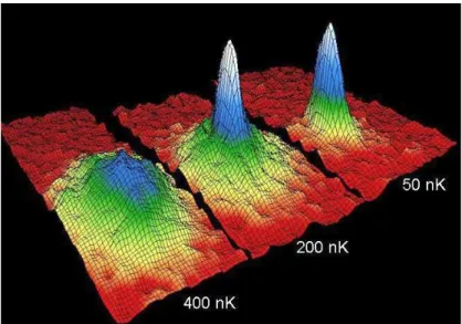
3 Einstein predicted BEC in 1924 [Ein25] after generalizing Bose’s new sta-tistical method of describing photons as entirely indistinguishable particles [Bos24]. London attributed the phenomenon of superfluidity in liquid helium to BEC in 1938. We know today that the interactions between particles in the liquid phase are too strong to condense more than 10 % of the particles. The experimental realization of BEC in weakly interacting systems re-quires advanced cooling and trapping techniques of low density atomic clouds. Three–body collisions that would cause classical condensation into solids or liquids are suppressed by keeping the gas dilute. Using laser and evaporative cooling, the temperature of the cloud is lowered by a factor of 109. In 1995, Andersonet al. achieved BEC in 87Rb [And95]. Figure 2 shows an absorption image of this first BEC. It illustrates the velocity distribution of an atomic cloud with a transition temperature TC ≈280 nK.
Figure 2: False–color images of the velocity distribution of an ultracold 87Rb cloud obtained by absorption imaging. The left most image shows the cloud just before the appearance of BEC, and the next just after the formation of BEC at TC ≈
280 nK. The right most shows a nearly pure condensate containing only 2000 atoms after further evaporative cooling had been applied. The circular pattern of the non–condensed fraction (mostly yellow and green) is an indication for the isotropic velocity distribution, which is consistent with thermal equilibrium. The condensate fraction (mostly blue and white) is elliptical and indicates a highly non–thermal velocity distribution. The peak is an image of a single, macroscopically occupied wavefunction. The field of view of each image is 200µm by 270µm [Ens98]. Figure taken from the JILA webpage http://jilawww.colorado.edu/bec/.
4
Today, Bose Einstein condensation, “a new window into the quantum world” [Ket99], is the basis of a whole field of new and exciting experiments and theories. Condensates of bosonic gases, mostly 87Rb, are routinely pro-duced in over 30 laboratories world–wide. BEC has long been achieved in all other stable alkali species, hydrogen, metastable 4He, and most recently,52Cr [Gri05]. BEC has been achieved with more than 105 molecules of Li
2 [Joc03] and also with fermionic atom pairs [Reg04]. This opens up the possibility to study the crossover from a BEC to a Bardeen–Cooper–Schrieffer (BCS) su-perfluid [Bar04]. The research into ultracold molecules, quantum information, and more fundamental research concerning the properties of both bosonic and fermionic ultracold gases continues at a breathtaking speed.
This diploma thesis contains two experimental projects, carried out in BEC laboratories in New Zealand and Austria. The first deals with the con-struction of a magnetic trapping apparatus, which is a key tool to achieve necessary phase–space densities for evaporative cooling. A short overview con-cerning the experimental realization of BEC is given in chapter 1. The second project focusses on the implementation of a frequency stabilization scheme of a ring–cavity laser. This laser is used for experiments with87Rb BECs in optical lattice potentials, where the transition from a BEC superfluid state to a Mott insulating state can be observed. A brief introduction to Mott insulators and the required optical lattice stability is presented in chapter 7.
Part I
Magnetic Trapping Apparatus
Otago, New Zealand
Chapter 1
Introduction
Trapping and storing of particles is key to scientific results in a large range of physics experiments. In the low–energy regime, advances in laser cooling and trapping paved the road to new experiments and the realization of Bose– Einstein condensation (BEC). The production of a BEC from a bosonic dilute gas requires multiple refined mechanisms to function in immediate succession. The crucial steps are described briefly in the following paragraph. Excellent reviews on most experimental aspects of BEC formation can be found in a review by W. Ketterleet al. [Ket99], and references therein.
To create a BEC in a dilute gas, approximately 109 bosonic atoms are isolated in an ultra–high vacuum (UHV) chamber and confined in a Magneto– Optical trap (MOT). This trap consists of counter–propagating laser beams at appropriate wavelengths and polarizations. Laser cooling (Nobel Prize 1997) in three dimensions is used to slow and effectively cool the atoms down to micro–Kelvin temperatures. The first MOT was developed in 1987 [Raa87], but attempts to create BEC with the use of optical cooling and trapping techniques alone fail, because the number and density of atoms is then limited by inelastic collisions and absorption of scattered laser light. Instead, the pre– cooled atomic cloud is loaded into a magnetic trap, where the necessary phase– space densities can be achieved. In the trap, an inhomogeneous magnetic field exerts a force on the magnetic dipole of the neutral atoms. This force depends on their internal state, leading to trapping of specific hyperfine states only. On a conceptual level, the magnetic trap acts similarly to a thermos flask, keeping the atomic ensemble tightly confined and providing the necessary densities to allow effective evaporative cooling. This cooling technique, which achieves the necessary phase–space densities, is illustrated in figure 1.1. Evaporation is performed by applying radio–frequency (rf) sweeps to the thermal cloud. By adequately ramping the resonant frequency, the hotter atoms are removed by
8 CHAPTER 1. INTRODUCTION inducing a transition to non–trapped hyperfine states. Resonant absorption depends on the magnitude of the magnetic field. Since the hot atoms populate different regions of the magnetic field than the colder ones, they can be removed selectively. Finally, the cloud effectively cools down due to rethermalization of the remaining atoms. The particle number depletes to about 105 and the critical temperature of approximately 100 nK is reached.
Figure 1.1: Illustration of evaporative cooling process in a magnetic trap. The deep trap contains hot and cold atoms. Hot atoms are ejected by rf–induced lowering of the trap. The ensemble cools down due to rethermalization. Figure courtesy of I. Bloch.
Magnetic traps are therefore a vital part towards reaching the necessary temperatures and densities for creating BEC: they isolate the atoms, keep them tightly compressed during evaporative cooling to achieve high collision rates, and finally hold the condensate for study. As evaporation is performed slowly (∼30 seconds), magnetic traps require low heating and loss rates.
When designing and constructing a magnetic trap, there are many basic configurations available that can be extended to an arbitrary degree. Gen-eral restrictions are imposed by the geometry of the coil or permanent magnet arrangement. Derived from the simple quadrupole trap, one of the pioneer-ing advances in the field was the invention of the QUIC (quadrupole–Ioffe– configuration) trap. It was developed by T. Esslinger et al. [Ess98] in 1998 and is now widely used.
In course of a project at the “Ultracold Atoms Research” Group at the University of Otago, and under the supervision of A. C. Wilson, I have planned, modelled and built a magnetic trapping apparatus of the QUIC type. Basic principles of magnetic trapping of neutral atoms and the outline of the QUIC trap are presented.
Chapter 2
Background and basics
Unlike charged particles, which are subject to the relatively strong Coulomb interaction and can be trapped in electric fields, neutral atoms display much smaller interactions with external fields. Attempts to trap them in solely static electric fields by inducing a dipole fail, because the atoms are attracted to re-gions of high field. As Laplace’s equation does not allow for a static local electric field maximum in free space, the atoms cannot be confined.
When placing neutral atoms into oscillating light fields or optical traps (e.g. standing wave) that are tuned near atomic transitions, they are subject to absorption and spontaneous emission of photons. The trap’s performance is restricted by the so–called recoil limit: the radiation force one photon recoil ex-erts on one atom limits the lowest achievable temperature of the atomic cloud to approximately 10µK. Optical dipole traps [Gri00], in contrast, employ far– detuned light and rely on the interaction of the electric dipole with the laser field. Dipole traps are used for achieving BEC, but they are generally shallow. The trap depth, which is defined as the temperature at which the atoms have sufficient kinetic energy to escape the trapping potential, is below one µK for optical dipole traps.
As magnetic forces are strongest for atoms with an unpaired electron, magnetic traps are a convenient starting point for successful BEC experi-ments using pre–cooled alkali atoms. A simple computation illustrates why pre–cooling of the atomic sample is important for the use of magnetic traps: consider the magnetic dipole moment of an alkali atom to be on the order of a Bohr magneton, µB. In order to produce a trap depth of 1 K, fields on the
order of 1.4 T are required. Temperatures of a fewµK are easily reached with 9
10 CHAPTER 2. BACKGROUND AND BASICS laser cooling and fields of only a few Gauss1 are sufficient to tightly confine the atoms.
Magnetic trapping has the advantage that, in the absence of near–resonant laser light, no excited states are populated and spontaneous emission cannot occur. The trap depth is large and typically amounts to 100 mK. Due to a considerable trapping volume, fast and efficient evaporation can be performed and studies of the BEC benefit from an improved signal–to–noise ratio. A disadvantage of this trapping method is its dependence on the internal state of the participating atoms. Experiments concerning the internal dynamics are limited to a few special cases.
2.1
Neutral atoms in magnetic fields
When an atom with a magnetic dipole moment is exposed to an external magnetic field, the dipole experiences a torque. This results in a magnetic potential energy shift ∆E, which is called Zeeman effect and can be written as
∆E =−~µ·B,~ (2.1)
where ~µis the magnetic moment of the atom and B~ the magnetic field. Neutral alkali atoms posses a large magnetic moment due to the single unpaired electron. In the case of 87Rb, the resulting magnetic moment ~µ is composed of the electron orbital and spin angular momenta, and contributions from the nucleus. The coupling between the angular momentum L~ of the outer electron and its spin angular momentum S~ results in a fine structure according to J~=L~ +S~. The hyperfine structure results from the coupling of the total electron angular momentum J~and the total nuclear momentum I~to the total angular momentumF~ =J~+I~. According to Bohr’s quantization rule that angular momenta exist only in integer and half–odd multiples of Planck’s constant ~, the magnetic moment ~µcan be written as
~µ=−gFµB(F /~ ~), (2.2)
where F /~ ~ is dimensionless and µB = e~/(2me) is the Bohr magneton. The gyro–magnetic ratio gF can be calculated with
gF =gJ ·
F(F + 1)−I(I+ 1) +J(J + 1)
2F(F + 1) , (2.3)
where for the 87Rb 52S
1/2 electronic ground state, the Land´e–factor gJ ≈ 2
[Ste01]. For a magnetic field in the z direction, we obtain equally spaced
1
Gauss is still commonly used and the conversion into the SI unit Tesla is 104
2.1. NEUTRAL ATOMS IN MAGNETIC FIELDS 11
energy levels
EmF =µBgFmFBz, (2.4)
which scale with the magnetic quantum number mF. As long as the energy
shift due to the magnetic field is small compared to the hyperfine splitting (which is on the order of 7 GHz for87Rb),F~2 andF
z commute with the
Hamil-ton operator, andF and mF are good quantum numbers. For given J,I, and
F, we can label the appropriate energy levels using mF.
Figure 2.1 shows the Zeeman splitting of the 52S
1/2 hyperfine ground state of 87Rb as calculated by the Breit–Rabi formula [Ste01, Eqn. (26)]. The ab-scissa shows the strength of the external magnetic field in two different regimes. The state is characterized byI = 3/2 andJ = 1/2 (due toL= 0 andS = 1/2), so that the total angular momenta of F = 1 and F = 2 are present. The gF–
factors are calculated using equation (2.3) to be −1/2 and +1/2, respectively. Figure 2.1 (a) illustrates two different regimes: according to the Zeeman effect
F is a good quantum number at low fields. In the region of the Paschen–Back effect at high fields on the right hand side, J is a good quantum number, and the grouping is done according to the appropriate quantum number mJ.
Figure 2.1 (b) shows the linear regime that we are interested in. With the magnetic trapping employed here, we are interested in the very left hand limit on both figures.
Trapping neutral atoms requires a local minimum of the magnetic energy potential in equation (2.4). As can be seen there, for gFmF >0, this requires
Bz to have a local magnetic field minimum. States which satisfy this condition,
are referred to as weak–field seekers. In contrast, the strong–field seeking states with gFmf < 0 cannot be trapped by static magnetic fields since Maxwell’s
equations do not allow for a magnetic–field maximum in free space. Referring to the ground state of 87Rb, the following states can be magnetically trapped:
|F = 2, mF = 2i with gF = +1/2
|F = 2, mF = 1i with gF = +1/2
|F = 1, mF =−1i with gF =−1/2
The other available states are either not trapped when mF = 0, or are even
anti–trapped for gFmF < 0. They escape the magnetic confinement and are
lost. The states where F = |mF| are trapped most strongly, and due to
their scattering properties, atoms in the largest F–state are favorable for the subsequent evaporation process.
When the atoms are trapped in a uniform magnetic field, the magnetic dipole precesses around the magnetic field direction with a constant angular
12 CHAPTER 2. BACKGROUND AND BASICS B, Gauss E n er gy / h , G H z 0 2000 4000 6000 8000 10000 -20 -15 -10 -5 0 5 10 15 20 F = 2 F = 1 mJ = +12 mJ =−12
(a) Paschen–Back regime.
B, Gauss E n er gy /h , G H z 0 200 400 600 800 1000 -6 -4 -2 0 2 4 F = 2,gF = +12 F = 1,gF =−12 mF = 2 mF = 1 mF = 0 mF =−1 mF =−2 mF =−1 mF = 0 mF = 1
(b) Anomalous Zeeman effect.
Figure 2.1: The87Rb 52S1/2 ground state energy (and the resulting hyperfine struc-ture) is shown as a function of an external magnetic field. In (a), the levels are grouped according to the value ofF in the low field regime (anomalous Zeeman ef-fect) and the value ofmJ in the strong field regime (Paschen–Back effect). In figure
(b), which shows the region of small fields, the levels are grouped according to F in the anomalous Zeeman effect regime.
2.2. QUADRUPOLE TRAP 13
frequency ωL. The Larmor frequency
ωL= µB ~ |B~|= e 2me| ~ B| (2.5)
describes the motion of the dipole. In an inhomogeneous field, the atom expe-riences a net force proportional to the magnitude of the magnetic moment
~
F =−µBgFmF∇|~ B~|. (2.6)
The rate at which the magnetic field is changed needs to be sufficiently small so that the magnetic dipole can follow the changing magnetic field adiabatically.
2.2
Quadrupole trap
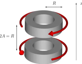
The most straightforward way to trap atoms magnetically is in a quadrupole field. This field is generated by two identical coils carrying equal currents running in opposite directions, as illustrated in figure 2.2. Near the center of the trap, the magnetic field is approximately homogeneous and its magnitude grows linearly with distance from the center, where it is zero. In this configu-ration, this field minimum is located at x=y=z = 0 and coincides with the symmetry center between the coils. In BEC experiments, both the thermal cloud and the condensate are smaller than 1 mm and we can safely assume only the linear field region to be of interest. This scheme was first employed in 1985 to trap sodium atoms [Mig85].
6x R 6 ? 2A=R
Figure 2.2: Coil configuration for a quadrupole trap. The direction of the current and spacing according to the Helmholtz configuration, 2A=R, is indicated.
14 CHAPTER 2. BACKGROUND AND BASICS The linear potential is characterized by the magnetic field gradient given as
Bx =Bx0x, By =By0y, Bz =Bz0z. (2.7)
Maxwell’s equations demand the sum of the gradients to be zero and assuming rotational symmetry about the x–axis, this coincides with B0 ≡ −B0
x/2 =
B0
y = Bz0. Hence, the gradients in the y– and z–direction are half of that in
x–direction. We obtain a spherical quadrupole field, which can be written as
~
B = (−2x, y, z)B0. (2.8) There is no axial field component in the plane defined by x= 0 and no radial field component on the x–axis.
y, cm x , cm -2 -1 0 1 2 -2 -1 0 1 2 y, cm z , cm -2 -1 0 1 2 -2 -1 0 1 2
Figure 2.3: Field magnitude of the quadrupole trap in thex–z–plane on the left and along the symmetry axis (x) for a quadrupole trap in Helmholtz configuration. For coils with the radiusR= 3 cm, spaced A= 1.5 cm, we obtain the shown symmetry, linear field variation near the trap center and a stronger gradient in the axial than the radial direction of the coil arrangement. Each contour line corresponds to a field increase of 0.5 G.
Figure 2.3 shows the field symmetry of the x–y–plane at z = 0 and cen-tered on the symmetry axis cut at x= 0 in contour plots. The even spacing of the potential lines near the trap center illustrate the linearity of the field gra-dients. The left hand plot illustrates the difference in axial and radial gradient for the quadrupole trap: along the symmetry axis of the two coils (x–axis), the gradient is twice as large as along the radial direction. The right hand plot illustrates the radial symmetry along the rotation axis of the quadrupole coils.
2.2. QUADRUPOLE TRAP 15
Staying close to the Helmholtz configuration ensures strongest confinement as the linear gradient is maximized [Mig85].
For stable trapping and successful cooling, the following condition needs to be fulfilled: the atom only remains trapped if its magnetic moment follows the magnetic field adiabatically. The Larmor frequency must be large compared to the rate of field change so that
dθ
dt ωL =
µB|B|
~ . (2.9)
An upper bound for the change of field rate dθ/dt is the trapping frequency, which is derived from the motion of the atom in the confining potential in equation (3.7) on page 24.
When cooling the atoms, they are forced towards the center of the quadru-pole trap, where the magnetic field amplitude is zero. As equation (2.5) shows, the Larmor frequency even vanishes for areas of B = 0, so that the adia-batic following condition in equation (2.9) is violated. The orientation of the magnetic dipole moment is lost and the atoms can undergo a non–adiabatic transition to a non–trapped hyperfine state and are ejected from the trap. This transition in regions of low magnetic field is referred to as Majorana spin–flip [Maj32]. Atoms that are already cooled to lower temperatures are most likely to be lost, as they populate the bottom of the trap. Consequently, the quadrupole trap ‘leaks’ cold atoms - the cloud effectively heats up due to rethermalization. Various approaches have been applied successfully to stop this trap loss. The three most widely used solutions are:
1. With the TOP (Time–Averaged Orbiting Potential) trap, a rotating homogeneous bias field B0 is added to the spherical quadrupole field. The frequency of the rotation must be larger than the orbiting frequency of the atoms, but much smaller than the Larmor frequency. The result is a harmonic potential that provides tight confinement [Pet95]. A TOP trap was used to create the first BEC at JILA [And95].
2. The optical plug makes use of optical dipole forces, and uses a tightly focussed and far blue detuned laser beam that forces atoms away from the trap center. Condensation of23Na was achieved using this technique at MIT in 1995 [Dav95].
3. The Ioffe–Pritchard (IP) traps originate from trapping schemes used for neutrons. They are characterized by a field minimumBmin >0 and a
harmonic potential near the trap center. They provide tight confinement for small clouds and feature large trap depths. The use for neutral atoms was first proposed by Pritchard [Pri84] in 1983 and IP traps are most
16 CHAPTER 2. BACKGROUND AND BASICS commonly used now. Details of this kind of trap are discussed in the following section 2.3.
2.3
Ioffe–Pritchard and QUIC trap
In the case of the quadrupole trap, the trapping potential rises linearly from the center of the trap, where the magnitude of the field is zero. As it is not possible to provide a non–zero magnetic potential with a linear field gradient, a harmonic potential is the tightest possible trapping potential that features a non–zero minimum. In the following, we consider a magnetic trap with a finite bias field along the z–direction and an axial field
Bz =B0+12Bz00z2. (2.10)
In first approximation, the transverse field component Bx is linear
Bx =B0x. (2.11)
If we now assume axial symmetry about thez–axis, applying Maxwell’s equa-tion yields a field configuraequa-tion [Ber87] that can be written as
~ B =B0 0 0 1 +B0 x −y 0 + B00 z 2 −xz −yz z2−1 2(x 2 +y2) . (2.12)
The minimum of the trap is located atx=y=z = 0, and the reference frame of the following equations is located around the potential minimum. The small thermal cloud or condensate, where2 k
BT < µBB0, is subject to a three– dimensional anisotropic harmonic oscillator potential. Usingρ2 =x2+y2, the potential is given by U =µBB0+ µB 2 B 00 ρρ2+Bz00z2 +O(x3, y3, z3, x2y, x2z· · ·), (2.13) where B00 ρ = B02 B0 − B00 z 2 (2.14)
is the radial curvature.
All IP traps feature a non–zero minimum, but there are many possible coil configurations. A list and their basic properties can be found in the Varenna
2
The magnetic moment µ of alkalis is on the order of a Bohr magneton µB, and for simplicity, we are usingµBB0 for energy estimates.
2.3. IOFFE–PRITCHARD AND QUIC TRAP 17
School notes by Ketterle et al. [Ket99]. Most of these macroscopic trap ar-rangements dissipate many kilowatts of power, unless they are constructed with supra–conducting coils. They require high current supplies when built with ordinary copper wire. Cooling, stabilization and switching become prob-lems and require creative solutions. Additionally, optical access to the atomic cloud as well as easy and reliable use are important considerations when de-signing a magnetic trapping apparatus. A special version of the IP trap, the QUIC trap, which consists of only three coils, provides successful solutions of these issues.
QUIC Trap
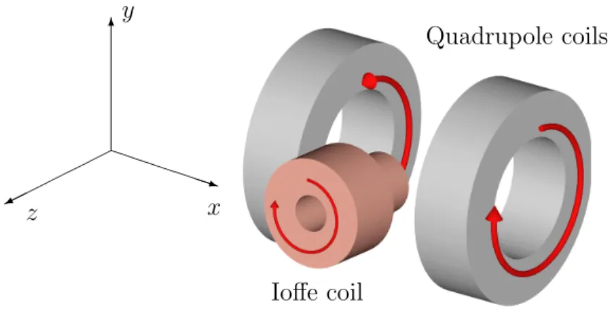
The QUIC (quadrupole–Ioffe–configuration) trap was introduced by T. Ess-linger et al. in 1998. It is characterized by its simple build, easy use, and low power dissipation [Ess98]. Optical access to the MOT, thermal cloud, and condensate is achieved more easily and without loss of tight confinement. A schematic setup of the three–coil arrangement is shown in figure 2.4.
6 PPPPP P q y z x Ioffe coil Quadrupole coils
Figure 2.4: Coil configuration for a QUIC trap. The axial direction refers to the
z–direction defined for the IP trap, which concurs with the symmetry axis of the Ioffe coil.
In this reference frame, the Ioffe coil is arranged along the z–axis, the quadrupole coils along thex–axis. The quadrupole field is produced with two coils running with opposite currents as described in section 2.2. In accordance with the mathematical expression derived earlier, the axial direction corre-sponds to the symmetry axis of the Ioffe coil, the z–direction in figure 2.4.
An important aspect for the successful implementation of an IP trap is the choice of bias field B0. Its value is crucial in terms of reducing losses while
18 CHAPTER 2. BACKGROUND AND BASICS keeping tight confinement.
The different trapping potentials for varying offset fields are plotted in figure 2.5, adapted from Ketterle et al.[Ket99]. A large bias field softens the potential in the radial direction. An over-compensating bias field causes zero crossings and Majorana spin flips along the trap axis. With a correctly tuned field, there are no zero crossings and radial confinement is tight.
x, y, cm | B − B0 | , G B0= 200 G z, cm | B − B0 | , G x, y, cm B0=−10 G z, cm x, y, cm B0= 2 G z, cm -1 0 1 -1 0 1 -1 0 1 -1 0 1 -1 0 1 -1 0 1 0 50 100 0 100 200 300 0 50 100 0 100 200 300 0 50 100 0 100 200 300
Figure 2.5: Bias field compensation is important for tight radial confinement in IP type traps. The illustrated magnetic field is characterized by a radial gradient of 300 G/cm, an axial curvature of 200 G/cm2, and three different bias fieldsB0. The upper row displays radial cuts, and the lower row axial cuts of the magnetic field profile. In the first column, radial confinement is softened as a result of the large bias field. The second column shows over-compensation by the bias field, resulting in two zero field crossings along the z-axis of the trap. In the third column, the bias field is tuned correctly, resulting in tight radial confinement and no zero field crossings. Adapted from [Ket99].
In the QUIC configuration, the confinement along z-axis is given by the field curvature of the Ioffe coil. The curvature scales with the current and radius of the coil asI/R3. Therefore, if the Ioffe coil can be placed close to the center of the quadrupole coils, tight confinement can be achieved with small radii and moderately low currents.
2.3. IOFFE–PRITCHARD AND QUIC TRAP 19
Within the modelling task of the project, we observed the change of trap-ping potential when the quadrupole potential is slowly changed into the QUIC arrangement. Experimentally, this is done by running a current through the quadrupole coils only and then increasing the current through the Ioffe coil from zero. This has practical applications as a loading scheme. Details on this can be found in section 3.3 on page 27.
Chapter 3
Modelling of QUIC trap
The main challenge in designing and building an easy–to–operate magnetic trap for the use in BEC experiments lies in balancing considerations such as physical space, power dissipation, and optical access with the best possible trap parameters such as the axial curvature, radial gradient, corresponding trapping frequencies, and aspect ratio of the trapping potential at low magnetic fields. During the course of the project the specifications of the physical space for the three coils changed tremendously. It evolved from the original idea to wind a small radius Ioffe coil from thin copper wire that would fit into a 1” diameter glass tube. This glass tube reaches into a vacuum chamber, ensuring close proximity between the coil to the center of a MOT arrangement, where the atoms are laser–cooled. Our results from the modelling revealed that the producible field parameters were well below our needs and expectations and the idea was therefore abandoned. Simultaneously, the 87Rb atom source planned for this new experimental setup was found to produce a deviating velocity dis-tribution, which put the feasibility of a Zeeman slower and described trapping arrangement in question.
Alternatively, a trap separated from the MOT and construction around a commercially available glass chamber (20 mm×20 mm×70 mm) is planned. The long direction is oriented horizontally. This arrangement is characterized by its flexibility, where loading schemes via magnetic transport over a succes-sion of quadrupole coils [Gre01], a moving quadrupole trap [Lew03], or push beam [Woh01] can be implemented.
In the course of the project I developed a suitable code for modelling the coil arrangement of the QUIC trap. Nick Thomas, a senior PhD student at Otago at the time, provided partial Matlab code he had previously written to calculate the magnetic field distributions of coaxial coils. All relevant code for modelling a QUIC trap is given in appendix A.
22 CHAPTER 3. MODELLING OF QUIC TRAP
3.1
Magnetic field from a loop
All calculations are based on the idea of stacking up closed wire loops and adding up the magnetic field every single one produces at a certain point in space. The magnetic field B~ from a single perfect loop with radius R
is calculated by integrating the vector potential A~ over the loop, and then applying ∇ ×A~ =B~. The field components can be calculated according to Bergeman et al. [Ber87]. For a coil orientated along the z–axis, centered at
z =A, and a current I, the field components are
Bz = µ0I 2π 1 [(R+ρ)2+ (z−A)2]1/2 h K(k2) + R2−ρ2−(z−A)2 (R−ρ)2+ (z−A)2E(k 2)i, (3.1) and Bρ = µ0I 2πρ z−A [(R+ρ)2+ (z−A)2]1/2 h −K(k2)+ R 2+ρ2+ (z−A)2 (R−ρ)2+ (z−A)2E(k 2)i, (3.2) and finally Bφ= 0. (3.3)
Here, Bz,Bρ, andBφare the axial, radial and azimuthal field components and
µ0 is the permeability of free space. Since we require axial field symmetry, there is no azimuthal field. K and E are the complete elliptic integrals with the argument
k2 = 4Rρ
(R+ρ)2+ (z−A)2. (3.4) These equations are used in the Matlab function b loop ex to compute
the magnetic field distribution far away from the origin. The conversion from cylindrical polar to Cartesian coordinates is performed with the func-tion coiloptions.
3.2
Characteristic parameters
There are three degrees of freedom for optimizing the coil arrangement and output parameters with the restriction of a given wire diameter dand current
I: the number of turns in each coil, their relative position, and the distance from the origin for the three coils.
Physically, the wire turns of a coil arrange as shown in figure 3.1. For simplicity, we use the indicated replacement picture and introduce an effective stacking distance in the radial direction of s=√3/2·d.
3.2. CHARACTERISTIC PARAMETERS 23
6
-rotational symmetry axis
ra d ia l d ir ec ti on
Physical wire stacking Replacement picture
Figure 3.1: Illustration of the change in the radial wire stacking pattern used for magnetic field model. The left image shows the physical situation, where the turns in the radial layers slip in between the space formed by the underlying layer. The right image picture shows what is implemented into the code: the diameter of the wiredremains the wire–to–wire distance along the rotational symmetry axis of the coil, and along the radial direction, it becomes s=dsin 60◦.
When designing the coil formers, the total height h of N turns in the radial direction is of interest. The height is calculated as
h=(N −1)·√3 2 + 1
·d (3.5)
wheredis the true wire diameter. Experience has shown that using more than 7 layers of standard wire (d∼2 mm) when only the inside turns are in contact with a cooling surface, is not advisable as the coils are likely to overheat.
The magnetic field along each axis is treated in the harmonic oscillator model as described in section 2.3. Along the z–axis, we use the harmonic approximation given by equation (2.10),
Bz =B0+12B00zz2, (3.6)
so that the axial curvatureB00
z is related to the trapping frequency ω using
µBBz00 = mω2. A larger curvature corresponds to tighter confinement and we
seek to maximize it, while keeping an offset field B0 ≈ 1 G. The trapping frequency ω is deduced for all three directions and the species in the trap, in our case87Rb. Withm
24 CHAPTER 3. MODELLING OF QUIC TRAP instance, yields U = 1 2µBB 00 zz2 = 1 2mRbω 2 zz2 ⇒ωz = µ BB00z mRb 1/2 , (3.7)
where the value of the Bohr magneton isµB = 9.274·10−24J/T. Typical
trap-ping frequencies are 2π×200 Hz in the radial (xand y), and 2π×20 Hz in the axial (z) direction.
The power consumptionfor the coils is calculated individually for each coil using
P =I2R =I2%l
Q, (3.8)
where % = 0.0175Ωmm2
m is the specific resistivity of copper at room tempera-ture, I the current, andl the length of the wire. The length is extracted from the input parameters coil radius and number of turns. The cross sectional area of the wire diameter d is Q =π(d/2)2. The power consumption is minimized and we anticipate a maximum of 500 W for all three coils combined, to be able to use only water cooling.
In the reference frame used for the coil arrangement in theMatlabmodel, the Ioffe coil is arranged along thez–axis and the pair of quadrupole coils along the x–axis. The origin of this reference frame is located at the center between the quadrupole coils. The position of the potential minimum of the QUIC trap is axially displaced towards the Ioffe coil by ˆz. We use fit functions around this minimum to extract the characterizing parameters introduced in this section. The position of the minimum, ˆz, along the z–axis of the trap is of interest in order to provide optical access to the condensate through the quadrupole coils. It can be influenced by allowing for a higher bias field and in return decreasing confinement.
The radial gradient near the trap center is derived from a Taylor expansion to second order, so that with ρ2 =x2 +y2
B =B0+ 1 2 B02 B0 − B00 z 2 ρ2+ 1 2B 00 zz2, (3.9) and Bρ00 = B02 B0 − B00 z 2 ⇒B 0 = s B0 B00 ρ+ B00 z 2 , (3.10)
3.3. COMPUTATIONAL RESULTS 25
where B0 the bias field, Bz00 the axial curvature, and Bρ00 the radial curvature.
The radial gradient B0, which corresponds to the stiffness of the trap, is
strongly influenced by the choice of bias fieldB0 as illustrated in figure 2.5 on page 18.
The anisotropy, or aspect ratio,λ, of the atomic cloud inside the trap is of interest, because the radial curvature is usually substantially larger than the axial curvature. Accordingly, the atomic cloud is cigar–shaped with the long axis along the trap’s z–axis. The aspect ratio scales as
λ= s B00 ρ B00 z . (3.11)
Since evaporative cooling becomes more effective with a moderately, not too large aspect ratio, we target a value 7≤λ≤12.
The geometric mean trapping frequency is given by ¯
ω = (ωxωyωz)1/3, (3.12)
and is a figure of merit for the trap, since the collision rate needed for evapo-ration increases proportional to ¯ω due to adiabatic compression [Ket99].
3.3
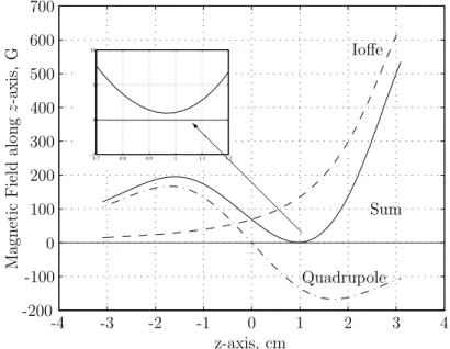
Computational results
The proposed coil arrangement is designed with the intention to allow opti-cal access to the field minimum both through the Ioffe coil and through the quadrupole coils. This allows probing of the condensate both in the vertical and the axial direction, and gives about 300◦ access in the y–z–plane. Optical
access to the origin of the reference frame, which is located at the center of the quadrupole coils, is easily implemented, as the x–axis coincides with the symmetry axis of the quadrupole coils. The schematic coil arrangement in figure 3.2 shows a cut aty = 0. The final trapping potential is shown in figure 3.3. It shows the axial magnetic field over a large region on the z–axis. The field produced by the quadrupole coils and the Ioffe coil are shown individually as well as the sum of both for a current ofI = 25 A through all three coils and a wire diameterd= 1.2 mm. The non–zero minimum is illustrated in the inset. The output parameters and results of the Matlab model of the pre-sented coil arrangement are summarized in the following table. Details and photographs of the constructed setup can be found in chapter 4.
26 CHAPTER 3. MODELLING OF QUIC TRAP z-axis, cm x -a x is , cm -4 -2 0 2 4 6 -4 -3 -2 -1 0 1 2 3 4 × -ˆ z glass cell
Figure 3.2: Cross section schematic of computed coil arrangement for QUIC trap cut at y = 0. The origin of the reference frame () and the approximate position of the magnetic field minimum (×) are indicated. The position and size of the glass cell is shown. The copper wire turns of diameterd= 1.2 mm are marked. The wire turns are stacked along their respective radial direction as indicated in figure 3.1.
z-axis, cm M ag n et ic F ie ld al on g z -a x is , G -4 -3 -2 -1 0 1 2 3 4 -200 -100 0 100 200 300 400 500 600 700 0.7 0.8 0.9 1 1.1 1.2 −5 0 5 10 @ @ @ @ @ @ @ @ I Ioffe Quadrupole Sum
Figure 3.3: The magnetic field component of Ioffe coil field, quadrupole field, and their sum is shown for I = 25 A. The inset illustrates the non–zero minimum (B0 = 0.93 G at ˆz= 0.96 cm) of the QUIC configuration.
3.3. COMPUTATIONAL RESULTS 27 Bias field B0 = 0.93 G Axial curvature B00 z = 204 G/cm2 Radial gradient B0 ρ = 147 G/cm Location of field
minimum from origin zˆ= 0.96 cm Total power dissipation P = 422 W Aspect ratio λ= 10.70
Trapping frequencies ωr = 194.8×2πHz
ωz = 18.3×2πHz
Geometric mean
trapping frequency ω¯ = 88.5×2πHz
Table 3.1: Output parameters of computed coil arrangement.
The Ioffe coil has a total of 102 turns, which vary in radius between 13 mm and 27.6 mm. The coil dissipates 124 W. It is located 31.07 mm from the center of the quadrupole coils. Thequadrupole coilsconsist of 160 turns each. The smallest turn has a radius of 13 mm, and the largest turn a radius of 17.8 mm. Each coil dissipates 149 W and the coil–to–coil distance is 32.2 mm (or origin to first turn 16.1 mm).
Transition to the QUIC configuration
We studied in detail how the trapping potential changes from the simple quadrupole to the QUIC trap when the current through the Ioffe coil is slowly increased at a fixed quadrupole current. This method finds experimental appli-cation in loading schemes from a Magneto–Optical trap (MOT) that contains pre–cooled atoms. Figure 3.4 displays the axial field magnitude and 3.5 shows the changing shape and position of the trapping potential in contour plots.
Figure 3.4 illustrates the magnetic field of the simple quadrupole trap along the z–axis that merges with a second magnetic field minimum, which is generated by the Ioffe coil, for increasing currents. In the process, the mini-mum moves along the axis towards the Ioffe coil and is lifted to non–zero field values1.
Figure 3.5 shows the process of the two merging magnetic field minima in contour plots for views at y = 0, which corresponds to a view from the top, and a cut atx = 0, the view through the quadrupole coils. In the first row of
1
28 CHAPTER 3. MODELLING OF QUIC TRAP -0.50 0 0.5 1 1.5 2 2.5 100 2000 100 2000 100 2000 100 2000 100 2000 100 200 M ag n et ic fi el d al on g z -a x is , G Ioffe current 0 A 10 A 15 A 20 A 22.5 A 25 A z-axis, cm
Figure 3.4: The magnetic field along the z–axis changes from the quadrupole to the QUIC configuration for increasing currents through the Ioffe coil. The current through the quadrupole coils is fixed at 25 A.
pictures, a current of I = 25 A runs only through the quadrupole coils. This produces a cone–shaped quadrupole field with a field minimum at zero as laid out in section 2.2 on page 13.
In the second row of plots, the current through the Ioffe coil is increased to 10 A. On the side where the Ioffe coil is positioned, a second quadrupole potential is forming on the symmetry axis of the Ioffe coil (z–axis). It ap-pears due to combination of the field gradients of the quadrupole and Ioffe configuration. It is visible in both plots that the long axes of the two potential minima are perpendicular to each other. For further increasing currents, the two potential minima merge and the overall cigar–shaped minimum is lifted up to B0 ≈1 G as illustrated in figure 3.3 on page 26.
The series of contour plots along the vertical axis in the left hand column display a Y–shaped potential for currents between 20 and 25 A. These trapping instabilities occur because the radial gradient is cancelled by the axial curva-ture [Ket99]. One needs to consider atoms escaping the trap at a certain axial displacement over the threshold. Since the objective is to trap laser–cooled
3.3. COMPUTATIONAL RESULTS 29 −0.5 0 0.5 −0.5 0 0.5 −0.5 0 0.5 −0.5 0 0.5 −0.5 0 0.5 −0.5 0 0.5 1 1.5 2 2.5 −0.5 0 0.5 z, cm −0.5 0 0.5 −0.5 0 0.5 −0.5 0 0.5 −0.5 0 0.5 −0.5 0 0.5 −0.5 0 0.5 1 1.5 2 2.5−0.5 0 0.5 z, cm x g z y g z I = 0 A I = 10 A I = 15 A I = 20 A I = 22.5 A I = 25 A View from top
at y= 0
View through quadrupole coils at x= 0 x , cm y, cm
Figure 3.5: The trapping potential changes from the quadrupole into the QUIC configuration. With a steady current through the quadrupole coils of 25 A, the current through the Ioffe coil is gradually increased as indicated. We observe the transition cut aty= 0 (left) and cut atx= 0 (right). Each contour line corresponds to an increase of 10 G in the magnetic field amplitude.
30 CHAPTER 3. MODELLING OF QUIC TRAP atoms, the barrier indicated by the contour lines is too high for the atoms to escape.
For the transition from the quadrupole to the Ioffe configuration, the gradient of the quadrupole field decreases along thex–axis and increases along the y–axis. Additional radial compression is not necessary. The potential displayed in the last rows of both figures 3.4 and 3.5 correspond to the final modelling result presented in this section.
Chapter 4
Experimental implementation
All coil formers and parts of the mounting system were constructed in the Mechanical Workshop in the Physics Department at Otago by Peter Stroud. They are made from aluminum alloy and all screws and bolts are, apart from plastic water fittings, metric. The copper wire used for winding the coils is insulated with an enamel coating and has a nominal outer diameter of 1.2 mm. The coating is reasonable sturdy, but scrapes off easily when in contact with sharp objects. All corners and edges of the formers are therefore carefully polished with metal files and fine sandpaper. Edges in direct contact with the wire are covered with Kapton tape, a high performance polyimide film that withstands high temperatures and is backed by a silicone adhesive. The space between the copper wires is filled up with heat–conducting silicone paste to improve heat transport.For the electrical connection, we use silver plated copper crimp contacts and single pole housings. They are approved for use up to currents of 30 A. Concerns over magnetic field switching stability dictate that the three coils should be connected in series. The one DC power supply available to us is from Agilent (Model E4356A) and delivers a maximum current of 30 A at up to 70 V. The laboratory features the necessary single phase outlet. We plan to use a maximum current of 25 A. The lack of a second power supply bears the disadvantage that the changeover from the quadrupole to the QUIC potential, which can find application as a loading scheme, illustrated in figure 3.5, can not be verified in scope of this thesis.
4.1
Magnetic field coils
The Ioffe coil follows the design of formers previously constructed at Otago. A schematic cross section and photographs are shown in figure 4.1 on page 33.
32 CHAPTER 4. EXPERIMENTAL IMPLEMENTATION The wire is wound onto a piece of aluminum alloy which has been hollowed out to allow water flow within. The former features three different sections separated by disks. Towards the origin of the reference frame, the radius of the wire turns decreases, as the turns further away from the point of interest at the origin only contribute to the magnetic field if their radius is sufficiently large. A slit along the axial direction prevents eddy currents when the current is turned off suddenly, as will be the case when conducting expansion of con-densates for time–of–flight (TOF) measurements. The slit widens towards the radial center and allows almost 6 mm of optical access along the z–axis as can be seen in figure 4.1.
In order to provide a large diameter hole to access the condensate vertically along the y–axis, the quadrupole coils are designed differently: the water– cooling is constructed to be on the outside of the former. This means that the outer turns of the coil, rather than the smaller ones on the inside, are indirectly water–cooled. The coil is wound onto a separate former, which is shown in figure 4.2 on page 34. A hollow tube is constrained by a disk in the front and back to prevent the wire slipping off. The center disk shown in the photograph in figure 4.2 is intended to improve the heat flux by providing an increased amount of contact area to the aluminum. It was removed during the winding process as it was impossible to wind a coil over two sections that would slide into the retainer without damage. At the cross–over point from one section to the next, the wire would protrude beyond all the other wire layers and the limiting disks on either side by approximately 1/4 mm. The insulation was rasped off the wire and coil was short–circuited.
The former fits tightly into the second piece, the retainer, which is shown in figure 4.3. It allows a water–flow around the former and prevents it from sliding after assembly. Both the former and the retainer are equipped with slits preventing eddy currents.
All coils are wound on a turning machine that ensures the wire is under tension at all times. For the first turn, a sharp 90◦ angle is formed with a well
padded tool to force the wire to run parallel to the confining disk. The first layer is generously covered in heat–conductive paste and it is added whenever appropriate. The last 1 1/2 turns are glued to the underlying layers using TorrSeal. This vacuum approved two–component epoxy is solvent–free and can be used at temperatures up to 120◦C. For a full cure, the coils are left to
4.1. MAGNETIC FIELD COILS 33 -z origin -water ?
eddy current slit
O-ring B B B B BBN optical access 6 ? 80 -6 Kapton tape
Figure 4.1: Schematic cross section, back and front view photograph of the Ioffe coil former. Eddy current slit, optical access, and dimensions are indicated. The origin relates to the center of the quadrupole coils. All dimensions in mm.
34 CHAPTER 4. EXPERIMENTAL IMPLEMENTATION
44
36
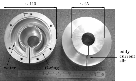
Figure 4.2: Former for the quadrupole coils. The photograph shows how the Kapton tape is applied to the edges only. ‘B’ and ‘T’ denote bottom and top coil. The schematic cross section shows the removal of the dividing disks. All dimensions are given in mm. ∼110 ∼65 -water O-ring A A
AAK eddycurrent
slit
Figure 4.3: Retainer for quadrupole coils in an inside and outside view. The inner section that accommodates the former measures∼39 mm across, the outer diameter of the lid side ∼110 mm. The groove for the rubber O–ring is indicated. The ruler in the bottom of the picture measures 170 mm. All dimensions are given in mm.
4.2. MOUNTING SYSTEM 35
4.2
Mounting System
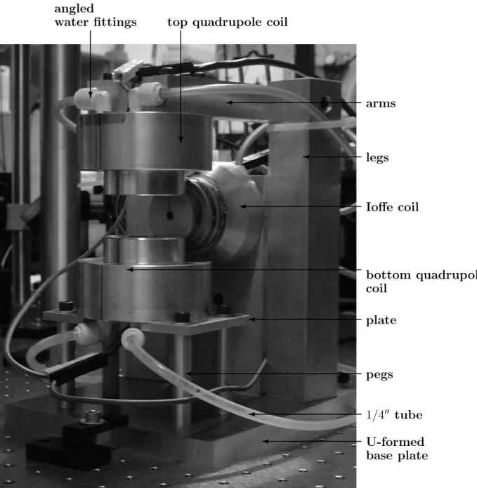
The mounting system can be seen on page 36. It is designed with the objective to provide an arrangement insusceptible to shocks caused by both mechanical influences and the current running through the coils. The compact mounting design of the quadrupole coils allows maximum optical access. All parts of the mounting system are constructed from (sandblasted) aluminum alloy. Care is taken to not block the optical access and only add solid pieces of aluminum where no eddy currents can develop.
The mounting of the Ioffe coil allows it to be moved in vertical direction with a clearance of±5 mm. In accordance with the typical beam height in the lab, the optical access is positioned 15 cm above the optical table. The lid of the coil is securely attached to the vertical piece of the mount. The base plate of the Ioffe coil mount rests on the laser table. The base plate can be moved closer towards the origin, but its movement is controlled by the U–formed base plate on which the quadrupole coils are attached.
The bottom quadrupole coil is secured on a plate and four pegs. The plate is equipped with appropriate clearings preventing eddy currents and providing optical access from below the trap. For adjustment of the height of the coil, the pegs can be removed and re–machined. The top quadrupole coil is suspended by a pair of legs and arms. The legs are the vertical bars, the arms the horizontal ones as marked in figure 4.4. The width of the arms can be adjusted to change the total height of the coil with respect to the bottom coil and laser table.
4.3
Water–cooling
All three coils are closed with plane aluminum alloy lids secured with multiple screws to the formers and retainers. Rubber O–rings close the coils water-tight. The grooves cut for the O–rings are visible in figures 4.1 and 4.3. They surround the water carrying volume. The edge that supports the O–ring is only a few millimeters thick, and therefore challenging to machine. Angled plastic water fittings connect the coils to a high pressure water supply with 1/400 plastic tubing. The threading of the water fittings are covered with
seal-ing Teflon tape. The water enters and exits the formers in close proximity to the eddy–current slits to create a large water flux and provide best possible cooling.
A distribution system made from a single aluminum block was planned but not finished within the time of the project. Filtered water will be piped to the laser table in one 12 mm tube, so that each coil is equipped with an
36 CHAPTER 4. EXPERIMENTAL IMPLEMENTATION U-formed base plate pegs plate bottom quadrupole coil legs arms ?
top quadrupole coil
Ioffe coil
?
angled
water fittings
1/400 tube
Figure 4.4: Mounting system of constructed QUIC trap with quadrupole coils in the foreground and Ioffe coil in the background. Note that the reference frame has been rotated for constructional reasons. The symmetry axis of the quadrupole coils is oriented vertically.
4.3. WATER–COOLING 37
individual circuit that can be locally interrupted. This facilitates effective and safe cooling and allows sufficient flexibility to position all tubing away from optical access to the trap.
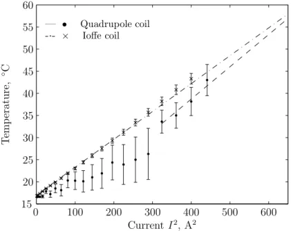
Temperature performance of coils
All three coils heat up with higher current flow. The performance of the (low pressure and provisional) water–cooling is tested for current induced temper-ature increase. As a precaution, the current is only ramped up to 20 A and interpolation performed for larger values. The surface temperature of the for-mers should not exceed 75◦C.
CurrentI2, A2 T em p er at u re , ◦ C 0 100 200 300 400 500 600 15 20 25 30 35 40 45 50 55 60 — • Quadrupole coil -·- × Ioffe coil
Figure 4.5: Measurement results for surface temperature dependence with increasing currents I2. Data for the Ioffe and one quadrupole coil is shown. The quadrupole data points at currents up to√300 A remain disregarded, as we are interested in the maximum surface temperature. The data points at higher currents are averaged over multiple probe positions. The linear approximations shows the surface temperature to remain below 60◦C when extrapolating to (25 A)2 = 625 A2.
The temperature probe, which consists of a two–metal contact, is attached to the hot regions of the formers using heat conducting silicone paste. For the Ioffe coil, this is the wire itself in the region where the largest number of coil turns is stacked. In the case of the quadrupole coil, we placed the probe halfway into the center clearance, which is the location furthest away from
38 CHAPTER 4. EXPERIMENTAL IMPLEMENTATION the water–cooling and closest to copper wire turns. The system is allowed to thermalize for 2 minutes at each current value.
Figure 4.5 illustrates the result for the coils. As the power consumption scales withP =I2R, we choose a linear display and can extrapolate, assuming constant cooling performance with the high–pressure water supply, to a maxi-mum surface temperature of 60◦C at 25 A for all three coils. The performance
Chapter 5
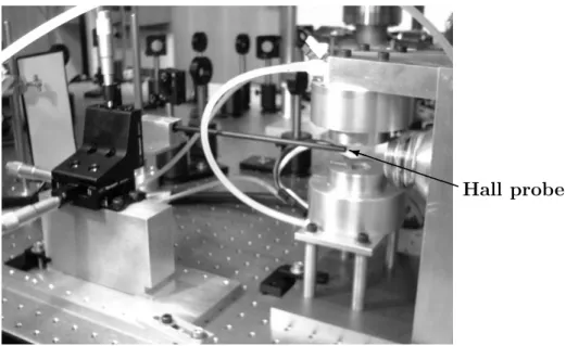
Verification of magnetic field
We measure the axial magnetic field of the quadrupole coils and the Ioffe coil individually and compare them to the modelled values. The results corroborate the model of the QUIC trap, but due to time constraints, the resulting overall magnetic field of the QUIC arrangement could not be verified. The field is mapped with a Gauss meter. The Hall probe is embedded near the tip of the approximately 20 cm long probe stick shown in figure 5.1. The stem is attached to a translation stage. P P P P P P P i Hall probe
Figure 5.1: Setup for field verifying measurements showing the mounted constructed coils and Hall probe on a translation stage.
40 CHAPTER 5. VERIFICATION OF MAGNETIC FIELD
5.1
Ioffe coil field
For the measurement of the Ioffe coil field, the probe is carefully adjusted along the symmetry axis of the coil. The total range of one data set is limited by the scope of the translation stage in the horizontal direction. The result of a typical measurement is shown in figure 5.2. For orientation, the Ioffe coil is positioned on the far right hand side of the figure and the z–axis zero corresponds to the center of the quadrupole coils. The distancea1, measuring from the origin to the first turn of the Ioffe coil, is the free parameter when comparing the measured values with the computational model. Analysis of the data using the model delivers a value of a1 = (32.8±0.3) mm. In the range of interest on the z–axis from 0 to 2 cm, the deviation in the magnetic field amplitude is less than 4 %.
z-axis, cm M ag n et ic fi el d , G -0.5 0 0.5 1 1.5 2 0 50 100 150 200 250 300 - a1 = 32.8±0.3 mm • Data points ?
Center of quad. coils
Figure 5.2: Measurement results of the axial magnetic field of the Ioffe coil. The
z–axis zero corresponds to the origin of the frame of reference, hence the center of the quadrupole coils. The data shows good agreement for the given a1, the origin to first turn distance.
On the physical setup, we measured a1 using calipers, and obtained a1 = (31.7±0.8) mm bearing a comparably large error, which is composed of the un-certainty of the position of the Hall probe inside the stem,δ= (0.38±0.25) mm, and the position of the first turn of the coil on the former. When assuming the overall shift of the data points on the z–axis to be on the order of±1 mm, we find that the level of consistency concerning the magnetic field values in the