This is a repository copy of
ML-NA: A Machine Learning based Node Performance
Analyzer Utilizing Straggler Statistics
.
White Rose Research Online URL for this paper:
http://eprints.whiterose.ac.uk/121681/
Version: Accepted Version
Proceedings Paper:
Ouyang, X, Wang, C, Yang, R et al. (3 more authors) (Accepted: 2017) ML-NA: A Machine
Learning based Node Performance Analyzer Utilizing Straggler Statistics. In: Proceedings
of the International Conference on Parallel and Distributed Systems - ICPADS.
International Conference on Parallel and Distributed Systems (ICPADS), 15-17 Dec 2017,
Shenzhen, China. IEEE . (In Press)
This is an author produced version of a paper accepted for publication in Proceedings of
the International Conference on Parallel and Distributed Systems - ICPADS . Personal use
of this material is permitted. Permission from IEEE must be obtained for all other users,
including reprinting/ republishing this material for advertising or promotional purposes,
creating new collective works for resale or redistribution to servers or lists, or reuse of any
copyrighted components of this work in other works. Uploaded in accordance with the
publisher’s self-archiving policy.
[email protected] https://eprints.whiterose.ac.uk/
Reuse
Unless indicated otherwise, fulltext items are protected by copyright with all rights reserved. The copyright exception in section 29 of the Copyright, Designs and Patents Act 1988 allows the making of a single copy solely for the purpose of non-commercial research or private study within the limits of fair dealing. The publisher or other rights-holder may allow further reproduction and re-use of this version - refer to the White Rose Research Online record for this item. Where records identify the publisher as the copyright holder, users can verify any specific terms of use on the publisher’s website.
Takedown
If you consider content in White Rose Research Online to be in breach of UK law, please notify us by
ML-NA: A Machine Learning based Node
Performance Analyzer Utilizing Straggler Statistics
Xue Ouyang
∗†, Changjian Wang
†, Renyu Yang
‡, Guogui Yang
†, Paul Townend
∗and Jie Xu
∗∗School of Computing, University of Leeds, UK
Email:{scxo, P.M.Townend, J.Xu}@leeds.ac.uk
†School of Computer, National University of Defense Technology, China
Email: c j [email protected], [email protected]
‡School of Computer Science and Engineering, Beihang University, China
Email: [email protected]
Abstract—Current Cloud clusters often consist of heteroge-neous machine nodes, which can trigger performance challenges such as the task straggler problem, whereby a small subset of parallel tasks running abnormally slower than the other sibling ones. The straggler problem leads to extended job response and deteriorates system throughput. Poor performance nodes are more likely to engender stragglers, and can undermine straggler mitigation effectiveness. For example, as the dominant mecha-nism for straggler alleviation, speculative execution functions by creating redundant task replicas on other machine nodes as soon as a straggler is detected. When speculative copies are assigned onto the poor performance nodes, it is hard for them to catch up with the stragglers compared to replicas run on fast nodes. And due to the fact that the performance heterogeneity is caused not only by static attribute variations such as physical capacity, but also dynamic characteristic uctuations such as contention level, analyzing node performance is important yet challenging. In this paper we develop ML-NA, a Machine Learning based Node performance Analyzer. By leveraging historical parallel tasks execution log data, ML-NA classies cluster nodes into different categories and predicts their performance in the near future as a scheduling guide to improve speculation effectiveness and minimize task straggler generation. We consider MapReduce as a representative framework to perform our analysis, and use the published OpenCloud trace as a case study to train and to evaluate our model. Results show that ML-NA can predict node performance categories with an average accuracy up to 92.86%.
Keywords—Node Performance, Straggler Problem, Machine Learning, Prediction.
I. INTRODUCTION
Task execution performance is important to both system managers and service users when applications are developed on parallel computing platforms such as Hadoop [1]. For the former, the delayed execution can lead to decreased system availability and potential SLA (Service Level Agreement) breakdown; while for the latter, the unpredicted response will result in poor user satisfaction.
It is common to witness node failures in large-scale pro-duction systems such as machine crashes, and methods to deal with node failures have been widely discussed. However, besides node failures, node performance degradation also calls for research attention, as it can lead to serious challenges such as the straggler problem. Straggler problem proposed by [2]
describes the phenomenon when a small subset of outlier tasks perform extremely slower than the other sibling tasks within the same parallel job. Speculator is a built-in component in Hadoop [3] to deal with the straggler problem. Upon straggler detection, a redundant replica task will be launched on another node for execution. The result generated by the quickest task will be adopted while the other task will then be killed.
There are multiple behaviors that can trigger the straggler generation within cluster environments, including hardware heterogeneity [4], resource contention [5], background net-work traffic [6], I/O discord [7], data skew [8] and OS or application-level related causes [9]. Among the possible reasons, node performance heterogeneity is an important one. In this paper, node performance refers to the node’s ability in terms of executing parallel applications.
Analyzing node performance is critical for straggler miti-gation, and machine learning techniques pose a bright shade onto it. Through classifying nodes into different categories and predicting the corresponding performance category with high accuracy, the scheduler can select suitable nodes to launch latency-sensitive tasks, avoid assigning speculative tasks onto nodes that are likely to be in their weak performance state in the near future. Our contributions are summarized as follows: • Analyzed node performance heterogeneity in a produc-tion cluster. With a case study of the OpenCloud system, we illustrate the straggler problem as well as how dif-ferent nodes affect straggler generation. In addition, we demonstrate the challenge of modeling such heterogene-ity, and show the necessity of leveraging task execution trace to measure nodes performance.
• Explored a series of features to describe node perfor-mance. These features are derived from task number per node values and statistics of normalized task executions. The former reflects the contention level while the latter captures relative processing speed of a node. A technique of conducting feature calculation in a time-incremental manner is developed to capture cumulative effects. • Proposed ML-NA, aMachineLearning basedNode
per-formanceAnalyzer. This multi-stage framework can clas-sify machine nodes into different categories depending on their performance through clustering. An automatic
labeling algorithm is developed in order to link the unsupervised learning with classification. Results show that, the average accuracy of using ML-NA to predict node performance category can reach as high as 92.86%. The rest of the paper is structured as follows: Section 2 presents the background; Section 3 proposes the ML-NA algorithm; Section 4 presents the prediction results and corresponding evaluations; Section 5 surveys the related work; Section 6 discusses the conclusion and the future work.
II. BACKGROUNDDESCRIPTION
In this section, the straggler problem will be discussed as well as the challenge of solving such problem caused by the node performance heterogeneity. All observations are based on data analytics results from the OpenCloud cluster.
A. OpenCloud Overview
OpenCloud is a research cluster at the Carnegie Mellon University [10] that consists of 116 machine nodes running Hadoop platform. The cluster supports research activities for different departments within the University. OpenCloud re-leased its task execution tracelog for public research covering the first nine months in 2012. There are 6 tables provided, from whichtask attempt historytable contains the information of interest, such as jobID, tasktype, taskID, start / shuffle / sort / finish time of the task attempt (represented as UTC timestamp in milliseconds), status (success, failed or killed), and hostname. After filtering, 18,935 successful parallel jobs consists of 8,734,974 tasks were analyzed within this paper.
In addition, the machine nodes within this cluster are homogeneous in physical configurations [10], with each has a 2.8 GHz dual quad core CPU (8 cores), 16 GB RAM, 10 Gbps Ethernet NIC, and four Seagate 7200 RPM SATA disk drives. However, in reality, due to dynamic operational situations and different aging conditions, the execution performance of these machines exhibits a diverse trend. This further results in the straggler problem that threats the timely and predictable service response and deteriorates system availability.
B. The Straggler Problem
In parallel computing frameworks such as Hadoop MapRe-duce [2], a job is divided into multiple subtasks running on
different nodes in order to achieve optimized response times. In this paper, Ti
j represents the ith task from job Jj, and
the cluster is composed of multiple machine nodesMm. The
scheduler is responsible for assigning tasks onto machines, whileDij denotes the duration ofT
i j.
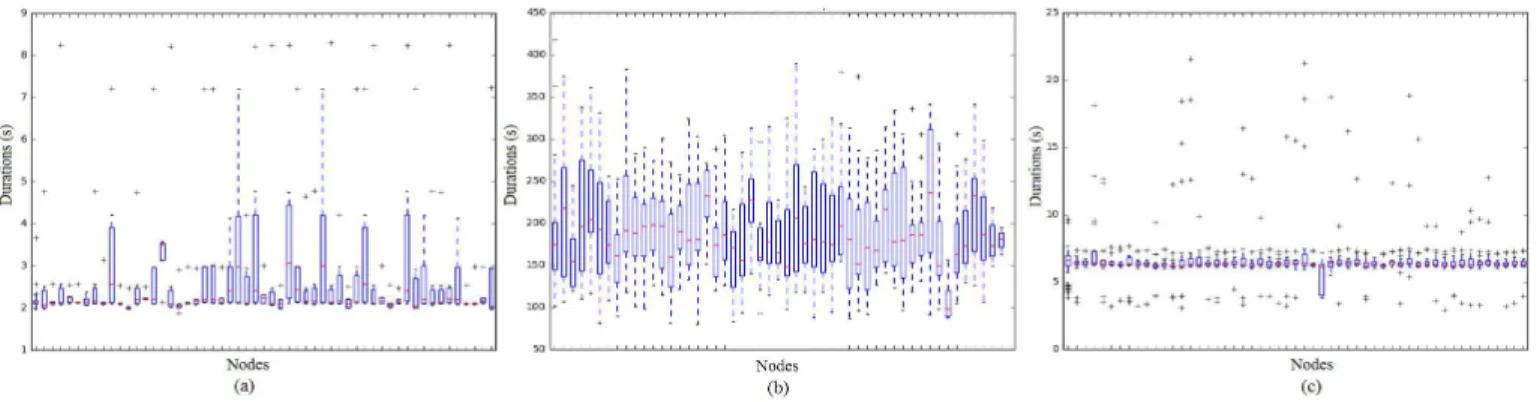
It is assumed that tasks from the same job have similar durations, such as the map tasks in the MapReduce framework. Theoretically, mappers in the same job should have similar execution lengths due to identical HDFS block size. However in practice, after being assigned onto different nodes, these subtasks vary in their durations. Figure 1 shows three examples of MapReduce jobs with different sizes in the OpenCloud cluster, consisting of (a) 366, (b) 805, and (c) 1116 mappers respectively. The straggler problem occurs when the duration variation is large enough that the extreme slow tasks under-mine overall job execution. In this paper, we define stragglers as tasks with estimated duration 50% larger than the average. This threshold is consistent with the majority of straggler mitigation literature such as [4] [6], and can be customized.
Stragglers occur due to resource contention, network con-gestion, input data skew, and most importantly, node per-formance heterogeneity. It is observable from Figure 1 that, with the red line representing the average duration for tasks assigned on each node from the same job, the ability for those nodes to execute parallel tasks are quite different. A few nodes incur more stragglers than the others, despite the fact that they have the same physical configurations.
C. Challenge: Node Execution Performance Heterogeneity
Node performance heterogeneity is one of the most impor-tant factors that lead to the straggler problem. This heterogene-ity is caused not only by physical capacheterogene-ity differences, but also system perturbations and partial upgrades. This section illustrates the challenge brought by such heterogeneity towards effective straggler toleration, and analyzed why the node performance analyzer is needed in order to mitigate stragglers.
1) Stragglers are not evenly distributed among cluster nodes: From task durations for different nodes shown in Figure 1, it is observable that some machines have a shorter average task processing time than the others, while some are either with a much longer average duration indicating a slower
execution, or with a larger variation in time of processing tasks, showing an unstable performance.
Figure 2 (a) illustrates the straggler number per node dis-tribution in the 9-month time, with machine IDs in each sub-figure remaining the same. That is to say, the blank machines in some sub-figures reflect the fact that not all nodes are in use for the whole time, some are only turned on in certain months. For example, nodes with ID∈(80,100]are used only in the 5th month. It is observable that, for each month, there
are some nodes experiencing much more stragglers than the others (labeled with circles in Figure 2 (a)). Considering the homogeneous physical configuration of the OpenCloud cluster, this shows that node performance is not purely dependent on their capacities. And to note that, the nodes with a significantly larger number of stragglers change over month, revealing a dynamic nature of straggler generation.
Related works such as [11] use resource utilization instead of physical capacity. However, the node performance diversity is not solely dependent on contention or utilization as well. Figure 2 (b) shows the total task number per node distribution over the 9-month time. The number of tasks assigned is used to partially represent contention level of the node due to the lack of utilization data. We see that, during each month, the task number for each node is relatively even. The 7th
month is the only exception, with three obvious busier nodes (labeled with circles). For the rest months, different straggler numbers are not due to contention. The node IDs in Figure 2 (b) are consistent through the 9 sub-graphs, same with Figure 2 (a).
2) The node performance is changing over time: Node performance in this paper refers to the node’s ability in terms of executing parallel applications, therefore it is reasonable to analyze node performance based on task durations. In Cloud environments, multiple workloads with different de-signed length co-exist with each other. For example, the job in Figure 1 (a) is less than 10 seconds while Figure 1 (b)
Fig. 3. Node Execution Performance Changing Trend
takes 450 seconds. That is to say, the raw task duration cannot directly be used to generate comparable results. To solve this problem, we proposed normalized execution value for tasks calculated in Equation (1) using the Z-score normalization.
f Di j= Di j−Dj σj (1)
In this way, the duration variation brought by job types can be eliminated. Dfi
j reveals the relative speed of t
i
j compared
to other tasks within Jj. A positive Dfij value represents a
slower execution because the duration ofti
j is larger than the
job average, and the increment of the positive Dfi
j indicates
an aggravated straggler behavior ti
j exhibits. Vice versa, a
negativeDfi
j indicates a shorter response, and the smaller the
negative value, the quickertij performs.
We then collect allDfi
j from tasks assigned in each node to
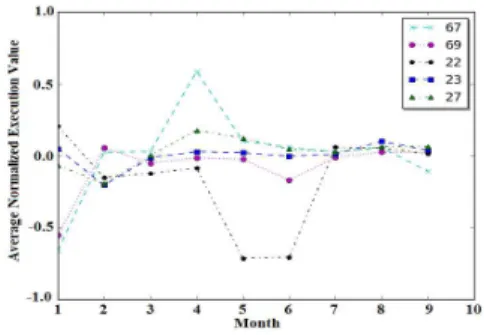
reflect the quickness or slowness derived from different node performance rather than job heterogeneity. Statistics of Dfi j
values per node are calculated as the basic metrics to measure the node performance. Figure 3 gives five nodes as an example. Each line in the graph represents a node, with y-axis being the Dfi
j average for the specific month. It is observable that
M22 outperforms the rest nodes in the5thand the6thmonth
though exhibiting a smaller negative average Dfi
j, while M67
has a noticeably worse performance among these five nodes in the 4th
month. Besides, there is no constant weak node throughout the 9-month time. For instance, M67 outperforms
the others in the 9th
month after it suffers in the4th
month.
3) Summary: As node performance is important in ensur-ing application timely response, to analyze its changensur-ing trend and make predictions based on historical patterns are vital in straggler mitigation. Machine learning techniques such as classification can be used to address the challenge of modeling such performance, with features reflected by the normalized workloads’ durations. In addition, the time series produced by the trace can be used to intelligently predict the performance changing trend. By investigating the machine learning based analyzer, we are able to capture the evolutionary behavior of nodes’ performance instead of simply using physical capacity nor contention indicators to determine a static performance.
III. ML-NA: A MACHINELEARNING BASEDNODE
PERFORMANCEANALYZER
In this section we propose ML-NA, a machine learning based node performance analyzer. Key processes of feature selection and automatic labeling are herein discussed.
A. Feature Selection
As we discussed in the previous sections, the node perfor-mance is typically influenced by multiple features, thus se-lecting key indicators to represent the node’s ability regarding parallel job execution is a vital process. In this paper, the parallel task execution trace is used to generate those key features. In particular, statistical attributes of the normalized task duration, task number, and timing attributes are adopted.
1) Statistical attributes: Node performance can be reflected by the statistical attributes of all tasks running on it within a certain time period. For example, if all tasks assigned to node M1 has an averageDfij of 2, we can infer that M1 is a
weak performance node because most tasks assigned on M1
are stragglers in their own jobs, characterized by2∗σj slower
than their own average duration Dj. And we can assume later
tasks that are about to be assigned onM1in the near future will
have a possible relative speed around 2∗σj times slower as
well. Other statistical attributes such as the standard deviation of allDfi
jpertaining to each node can also be used to reflect the
fluctuation range of the node performance, showing a stable or random possibility ofDfi
j in the certain node.
2) Task number: Apart from the statistical attributes de-rived from the Dfi
j distribution per node, task number is the
other important feature that we use to describe the node performance. It implies the node’s contention state and reflects the impact of such contention toward job execution rapidness. In addition, the normalized task number compared with all the other machine nodes in the cluster is used rather than the raw task number. This is because we intend to constrain the se-lected features into a similar range, which lays the foundation for further operations such as the clustering process.
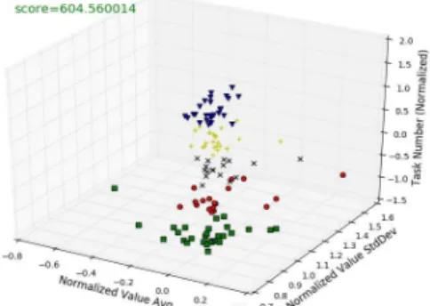
Fig. 4. Clustering Results with Three Features (k= 5)
The three basic meta-features selected to build up the node performance analysis model are the average and the standard deviation of all Dfi
js from tasks per node, as well as the
normalized task number. An example of leveraging these three meta-features to clustering nodes into 5 categories using k -means [12] is shown in Figure 4. Machine nodes within the same clusterization group have similar execution performance.
3) Timing attributes: Considering the fact that sometimes performance degradation is caused by time-cumulative im-pacts, ML-NA adopted another feature dimension: timing attributes. To be specific, we divided the trace into 9 month
according to the job submission time. Eachmonthcontains 30 days’ data (ignoring the fact that natural months are slightly different in day numbers). Within each month, we construct the input into dataset consists of following 91-tuples:
<Mid, avg{Dfij day1}, σ{Dfj dayi 1}, norm{N taskday1},
avg{Dfi
j day2}, σ{Df
i
j day2}, norm{N taskday2},· · ·,
avg{Dfi
j day30}, σ{
f
Di
j day30}, norm{N taskday30}>
Within this 91-tuple, avg{Dfi
j day1} and σ{Df
i
j day1}
repre-sent the average and the standard deviation of all tasks’ normalized value assigned onto the machine Mid in day1;
norm{N taskday1} stands for the normalized task number
on machine Mid compared with all other nodes within the
cluster in day1. To note that, avg{Dfi
j day2}, σ{Df
i
j day2}, and
norm{N taskday2}are calculated based on all tasks submitted
in both day1 and day2 together rather than day2 itself. In other words, this timing attribute calculation is performed in a cumulative manner. Similarly for day30, the results are derived from the whole month’s data rather than a single day.
B. The Automatic Labeling Algorithm
A labeling process is required by ML-NA because the trace data does not contain node performance indicators, while the labeled data is needed in order to train the classification model. Previously to label a weak node is a manual process that depends on the system administrator. In ML-NA, we proposed an automatic labeling algorithm that utilizes the generated features to objectively discriminate weak performance nodes from the normal ones within the cluster.
1) Clustering: The first step to label the nodes is to put the nodes with similar performance into the same group. In this scenario, clustering is the most well-known technique that can be used, and k-means is one of the simplest whilst very effective clustering algorithms [12].
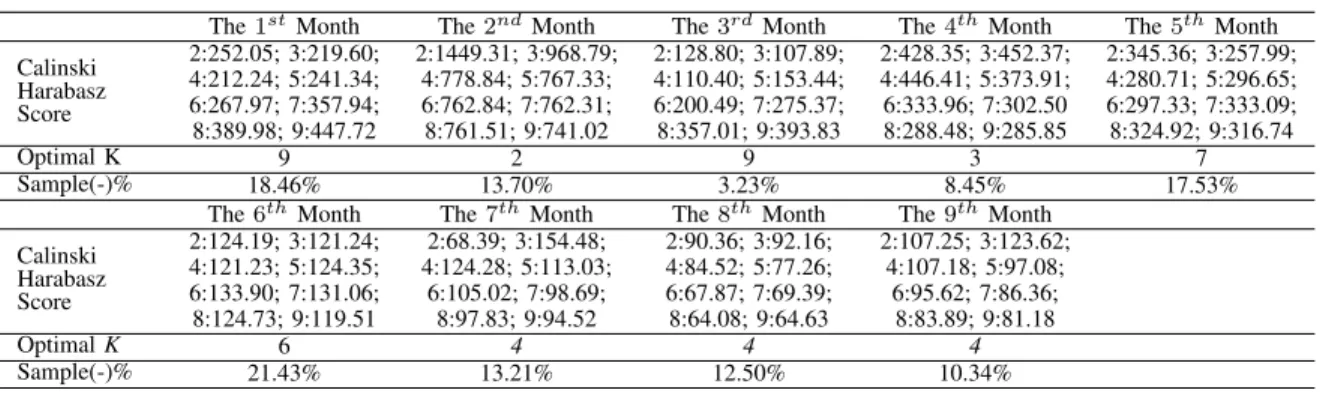
The key parameter for launching k-means is to find the optimal k value: it should be sufficiently large to reduce the number of nodes within each group, so that we can separate the minority (weak performance nodes) from the majority (the normal ones), yet maintaining the best clustering results such as high calinski-harabaz score [13]. The calinski-harabaz score measures the covariance within each cluster and the covari-ance among different clusters. Higher calinski-harabaz score signifies a superior clustering result. Figure 5 demonstrates the score variation whenkis changing from 2 to 10 using only two attributes to represent node performance. In this example, for the clarity of figure description, only two features are included, while in ML-NA, 90 features (exceptMid in the 91-tuple) are
used in order to conduct the clustering.
Table I details the calinski-harabaz scores whenkis ranging from 2 to 10 for each month. In this paper we specify the maximum clustering number to be 10 when exploring the optimalkbased on the observation that desirable proportion of weak performance nodes can be sorted out. This number can be easily customized according to different purposes. From the table it is observable that most optimal ks are the ones with the highest score. However, for the7th,8thand9thmonth, the
optimalkis different. This is due to the optimalkgenerated by the score is not big enough to differentiate a proper proportion of “weak” nodes set (leading to a negative sample percentage above 25%). Under this circumstance, the second largest score with a greater kwill be chosen.
2) Labeling: After putting the nodes with similar per-formance into k groups, we then need to determine which cluster represents the weakest performance group. Conven-tional labeling needs manual practice conducted by the system administrator, which suffers from operational inefficiency, and the subjective may lead to misidentification. To cope with it, an automatic labeling algorithm is proposed in ML-NA. Two heuristic ranking criteria are adopted to make this decision:
• [C1]: The weakest performance nodes should have the
Fig. 5. DifferentKClustering Results with Two Features
most number of positiveavg{Dfi
j dayN} (N∈[1,30]). The number of positive avg{Dfi
j dayN} is the primary
indicator when judging whether a specific group contains weak performance nodes. According to Equation (1), a positiveDfi
jsignifies a straggler. Therefore, for nodeMid,
a positive avg{Dfi
j dayN} indicates a high likelihood of
straggler occurance. As a result, the number of positive
avg{Dfi
j dayN} can be used to imply the frequency of the
node to exhibit such slow tendencies in a month time. • [C2]: If multiple cluster centers have the same number
of positive avg{Dfj dayNi }, then smallest σ{Dfj dayNi } suggests the worst performance(N ∈[1,30]).
The σ{Dfi
j dayN} value implies the confidence when
pre-dicting node performance, because it represents a stable or random status. A smallσ{Dfi
j dayN}indicates a
concen-tratedDfi
j distribution for nodeMid. Thus, for nodes that
have already shown a slow tendency (e.g. with maximum positiveavg{Dfi
j dayN}number according to [C1]), smaller
averageσ{Dfi
j dayN}means a higher chance for this group
to be classified as the weakest type.
The labeling algorithm is presented in Algorithm 1 follow-ing the above two heuristics. Label “1” represents the negative
TABLE I THEKVALUECHOICES
The1stMonth The2ndMonth The3rdMonth The4thMonth The5thMonth
Calinski Harabasz Score 2:252.05; 3:219.60; 2:1449.31; 3:968.79; 2:128.80; 3:107.89; 2:428.35; 3:452.37; 2:345.36; 3:257.99; 4:212.24; 5:241.34; 4:778.84; 5:767.33; 4:110.40; 5:153.44; 4:446.41; 5:373.91; 4:280.71; 5:296.65; 6:267.97; 7:357.94; 6:762.84; 7:762.31; 6:200.49; 7:275.37; 6:333.96; 7:302.50 6:297.33; 7:333.09; 8:389.98; 9:447.72 8:761.51; 9:741.02 8:357.01; 9:393.83 8:288.48; 9:285.85 8:324.92; 9:316.74 Optimal K 9 2 9 3 7 Sample(-)% 18.46% 13.70% 3.23% 8.45% 17.53%
The6thMonth The7thMonth The8thMonth The9thMonth
Calinski Harabasz Score 2:124.19; 3:121.24; 2:68.39; 3:154.48; 2:90.36; 3:92.16; 2:107.25; 3:123.62; 4:121.23; 5:124.35; 4:124.28; 5:113.03; 4:84.52; 5:77.26; 4:107.18; 5:97.08; 6:133.90; 7:131.06; 6:105.02; 7:98.69; 6:67.87; 7:69.39; 6:95.62; 7:86.36; 8:124.73; 9:119.51 8:97.83; 9:94.52 8:64.08; 9:64.63 8:83.89; 9:81.18 OptimalK 6 4 4 4 Sample(-)% 21.43% 13.21% 12.50% 10.34%
ALGORITHM 1: Labeling Algorithm Inputs:
Training setsdata={hMid, Avgday1,..., Numday30i}
OptimalKfromK-means process Output:
Labelled sets{hLabel, Mid, Avgday1,..., Numday30i}
1 Categories = kmeans(n clusters =K, data =data); 2 foreach center in Categoriesdo
3 for Avgdayj, StDevdayj in center.AttributeListdo
4 pos counts = count the number of j, Avgdayj >0
5 stdev avg = calculate the average of StDevdayj
6 end
7 end
8 WeakIndexList = Categories.indexof max(pos counts); 9 WeakIndex = WeakIndexList.indexof min(stdev avg); 10 foreach node in datado
11 ifCategory(node) == Categories.indexof(WeakIndex)then 12 Label = 1; 13 else 14 Label = 0; 15 end 16 node = node.insert(Label); 17 end 18 returndata
sample of weak nodes, and “0” indicates the positive sample of nodes that exhibit normal performance. To note that, the primary purpose of this paper is to model and predict the weak nodes to avoid straggler generation, therefore binary labels are adopted. According to different usage, a set of labels corresponds to multiple performance levels can be adopted.
IV. NODEPERFORMANCECLASSIFICATIONPREDICTION
ML-NA is a multi-stage learning procedure that predicts node performance based on classification while labeled data is fed into the classifier as input. This section details the node performance category classification and prediction results.
A. Boosting Based Classifier
There are a lot of classification algorithms [12] such as SVM, Boosting, Decision Tree, Random Forest, and Naive Bayes, etc. Each algorithm emphasizes specific attributes from the training data to get the optimal performance. For example, the Bayesian classifier requires all the attributes to be independent of each other (the attributes xk should fulfill
Equation (2), with Ci to be a given condition). P(X|Ci) =
n
Y
k=1
P(xk|Ci) =P(x1|Ci)×...×P(xn|Ci) (2)
Table II shows the precision, recall and accuracy when adopting different prevailing classification algorithms onto the OpenCloud datasets with automatic labeling to predict performance category. Parameters used are the default value in the Python scikit-learn library [13], and the cross-validation portion is 1/3. It is observable that the Naive Bayes classifier performs significantly worse than others. This is because, in our training set, the features (elements in the 91-tuple except Mid) are correlated (i.e., they are generated in an
incremental manner according to time). This is consistent with the aforementioned limitation of the Bayesian classifier. Within this paper, XGBoost [14] is adopted to realize the classification analysis.
TABLE II ALGORITHMCOMPARISIONS
Precision Recall Accuracy Random Forest 89.47% 58.62% 92.86% SVM 100% 6.9% 86.22% Ada Boosting 78.95% 51.72% 90.82% Decision Tree 62.96% 58.62% 88.78% Naive Bayes 16.67% 27.59% 68.88% XGBoost 82.61% 65.52% 92.86%
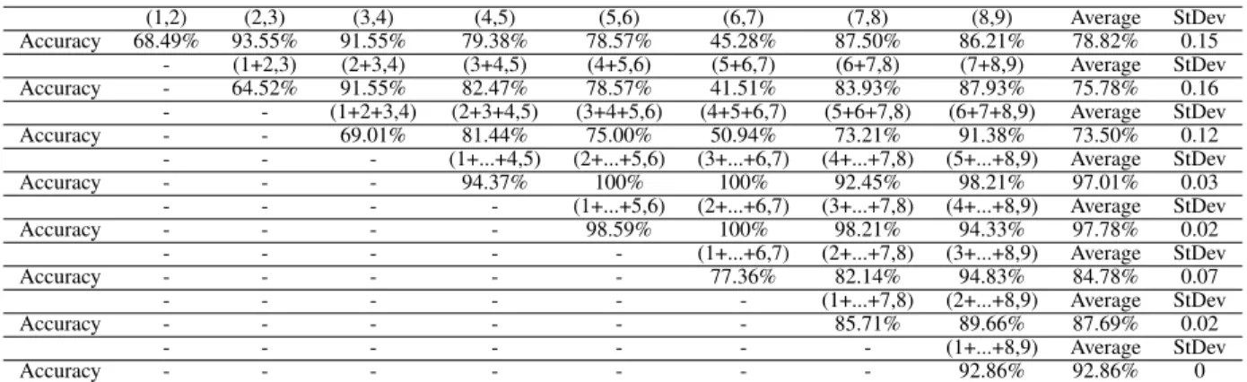
B. Prediction Results and Evaluations
Different parameter settings are tested to train the XGBoost model, main parameters tuned are learning rate η, evaluation metric, and gbtree depth. Table III detailed the optimal pre-diction result from all testing cases, with η being 0.1 and the maximum depth of the gbtree booster being 12. The
loglossvalue calculates the negative log-likelihood is adopted as the evaluation metric. The results of different data sizes are compared in the form of a sliding window to test the sensitiveness towards training sizes. For example, (1,2) in Table III represents the prediction result for node performance category in the 2nd
month through using training data in the
1st
month. Additionally, (1+...+8,9) represents the prediction result for the 9th
month by using a combined training data from the1st to the 8th month (a much larger training size).
The numbers in Table III are prediction accuracies cal-culated following Equation (3), where TP stands for true positive, TN is short for true negative. Similarly, FP and FN are abbreviations of false positive and false negative respectively. The average and standard deviation of accuracies for each training size are recorded in the table as well.
Accuracy= T P+T N
T P+F N+F P+T N (3)
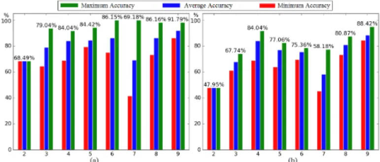
Figure 6(a) concludes the minimal, average and maximum accuracies when predicting each month’s node performance categories utilizing different training sizes with the optimal parameter setting. Figure 6(b) shows a example of results from another parameter setting, withη = 0.3, gbtree depth being 9, anderror represents classification error rate being the evalu-ation metric. The numbers listed in the figure are the average values, and it is observable that, the parameter settings in Table III surpasses the other testing case with much higher prediction
Fig. 6. Node Classification Prediction Accuracy for Each Month, with (a) Optimal Parameters used in Table III, and (b) Comparable Parameter Settings.
TABLE III
MODELPREDICTIONRESULTS WITHPARAMETERSETS OFη= 0.1,MAX DEPTH= 12,EVAL METRIC=LOGLOSS
(1,2) (2,3) (3,4) (4,5) (5,6) (6,7) (7,8) (8,9) Average StDev Accuracy 68.49% 93.55% 91.55% 79.38% 78.57% 45.28% 87.50% 86.21% 78.82% 0.15 - (1+2,3) (2+3,4) (3+4,5) (4+5,6) (5+6,7) (6+7,8) (7+8,9) Average StDev Accuracy - 64.52% 91.55% 82.47% 78.57% 41.51% 83.93% 87.93% 75.78% 0.16 - - (1+2+3,4) (2+3+4,5) (3+4+5,6) (4+5+6,7) (5+6+7,8) (6+7+8,9) Average StDev Accuracy - - 69.01% 81.44% 75.00% 50.94% 73.21% 91.38% 73.50% 0.12 - - - (1+...+4,5) (2+...+5,6) (3+...+6,7) (4+...+7,8) (5+...+8,9) Average StDev Accuracy - - - 94.37% 100% 100% 92.45% 98.21% 97.01% 0.03 - - - - (1+...+5,6) (2+...+6,7) (3+...+7,8) (4+...+8,9) Average StDev Accuracy - - - - 98.59% 100% 98.21% 94.33% 97.78% 0.02 - - - (1+...+6,7) (2+...+7,8) (3+...+8,9) Average StDev Accuracy - - - 77.36% 82.14% 94.83% 84.78% 0.07 - - - (1+...+7,8) (2+...+8,9) Average StDev Accuracy - - - 85.71% 89.66% 87.69% 0.02 - - - (1+...+8,9) Average StDev Accuracy - - - 92.86% 92.86% 0
accuracy. With proper parameter tuning, the prediction results for most months exceed 85%, and with proper training sizes, the highest prediction results for most months are above 90%. Under some cases, the highest accuracy when predicting next month’s node performance category even reaches 100%.
Despite the peak accuracy ML-NA can achieve, there are still some low accuracy results under extreme cases. The worst results occur when predicting node classification for the 2nd
and the 7th
month. The reason behind the low accuracy for the 2nd month is relatively straight forward - the insufficient
training size. When predicting the node categories for the2nd
month, we can merely collect data from the1stmonth. In fact,
the prediction accuracy based on only one month’s training data tends to be limited for most months. The numbers are shown in the first row in Table III. Most accuracies are below 80% such as the prediction pair of (1,2), (4,5), (5,6), and (6,7). For the low accuracy occur in the7thmonth, it is due to the
special characteristics of the input data. Figure 7 shows the first 10 lines for the training set, from which we see that, features
avg{Dfi
j day1},σ{
f
Di
j day1}, andnorm{N taskday1}toavg{
f
Di j day3},
σ{Dfi
j day3}, and norm{N taskday3} in the 91-tuple are NaN.
This is due to that, for the first three days of the 7th
month, there are no tasks been submitted to the system, leading to a blank value for those feature columns. These unexpected NaNs form a noticeable different pattern, leading to a low prediction accuracy for the classification model generated by ML-NA.
This result reveals a limitation of the proposed ML-NA algorithm: it can only predict node performance with high accuracy when there are jobs running in the system. Sudden reduce in task numbers may influence the algorithm perfor-mance. However, we believe this is a loose assumption that most production cluster can achieve.
Fig. 7. Training/Evaluation Segment for the7thMonth with NaN Attributes
V. RELATEDWORK
Mitigating stragglers has become an important challenge in improving parallel job performance, especially consider-ing the fact that most production clusters are composed of heterogeneous machines. The straggler problem is observed when a small subset of parallelized tasks performing much slower in comparison with other sibling tasks from the same job, incurring a significant delay towards final job completion. Stragglers stem from numerous causes including hardware het-erogeneity [4], resource contention [5], network traffic [6], I/O discord [7], data skew [8] and application related sources [9]. There are numerous work that analyzes the straggler influ-ence toward system performance: Jeffrey et al. [15] demon-strate that the slowest 5% of completed requests are responsi-ble for half of the total99thpercentile latency, and there exists
a positive correlation between straggler probability and cluster size, concluding that the possibility of longer latency will increase with the growth of system scales. Ananthanarayanan et al. [6] show that 80% of stragglers exhibit a delay between 150%-250% compared to the median duration, with 10% exhibiting a larger than 10 times response slowdown.
Among the straggler mitigation techniques, speculation [16] is the dominant method. It predicts stragglers based on task progress score and launch redundant copies for re-execution on different machines. LATE [4] is the most widely used speculation based method that designed for heterogeneous environments. It uses estimated duration as the metric to measure stragglers rather than progress score. MARLA [17] is also designed for heterogeneous clusters, re-configures MapReduce through delaying the binding of data to worker process. Some speculation variations use machine learning in revealing the correlation between task execution time and node level statistics such as the CPU/memory utilization. In [11], the historical data on each node is used to predict the possibility of stragglers through performing regression, while [18] presents a slowdown predictor using machine learning to forecast how much slower a task will run compared to similar tasks. Wran-gler [19] predicts stragWran-glers using linear modeling based on cluster resource usage counters, and [20] further enhances the
time-consuming data collection process of Wrangler through proposing multi-task learning formulations.
Current straggler mitigation techniques are focused more on application perspective, selecting the best task candidates to create the replications, however, ignoring the impact of nodes. In reality, node performance plays a vital role in straggler generation. Xu et al. [21] report that poor response time in EC2 is a property of nodes, and this property is both pervasive throughout EC2 and persistent over time. Therefore, it is particularly important to avoid scheduling speculative tasks to the nodes that are about to experience performance fall. [22] proposes a node performance ranking algorithm that identifies 0.83% of weakest nodes within Google cluster based on job execution. However, this method is offline analysis and does not generate a prediction that can guide future task assignment. In terms of intelligent placement of replicas on nodes, Chen et al. [7] consider both data locality and data skew, develop a cost-benefit model based on the load of a cluster. This method leverages data analytics to identify weak nodes, but it as-sumes node performance is a static characteristic that remains constant within the cluster, while transient system conditions including resource contention level, workload heterogeneity and user demand will actually influence the performance of the node to fluctuate over time.
VI. CONCLUSION
Analyzing and predicting node performance is important in guaranteeing efficient job execution. It facilitates the de-ployment of tasks by avoiding assigning them to the node that is likely to be in its weak performance phase in the near future. For straggler mitigation mechanisms such as speculative execution, it provides a guidance on the suitable node candidates that are ideal for launching replications. The main contributions of this paper are summarized as follows.
Firstly, we analyzed the node performance heterogeneity based on the OpenCloud tracelog data regarding parallel task execution. Different from literature that purely focuses on either physical capacity differences or utilization variations, we describe and measure the nodes’ performance using straggler statistics, which directly reflect the influence the heterogeneity exert on efficient job responses. Secondly, we explored a series of features to describe node performance and developed an automatic labeling algorithm to generate accurate and objective labels for different performance categories. Through leveraging normalized task execution times and task number per node values, statistical characteristics and timing attributes, we calculated the features to capture node execution ability. Finally, we proposed ML-NA, the node performance analy-sis framework that classifies machine nodes into categories. Prediction results show that ML-NA is capable of predicting node performance categories with an average accuracy up to 92.86%. This can further benefit the scheduler via blacklisting nodes that are likely to be in their weak performance state in the following scheduling window.
Besides above contributions, future works including inte-grating the proposed ML-NA algorithm into cluster scheduling
decision-making components such as the resource manager in YARN system. And to improve its ability in handling limitation situation when no tasks are submitted.
ACKNOWLEDGMENT
This work is supported by the China National Key Re-search and Development Program No. 2016YFB1000101, 2016YFB1000103, Chinese National Science and Technology Major Project No. 2016zx01040101-001, and Beijing BDBC innovation center.
REFERENCES
[1] M. Garc´ıa-Valls, T. Cucinotta, and C. Lu, “Challenges in real-time virtualization and predictable cloud computing,” Journal of Systems Architecture, vol. 60, no. 9, pp. 726–740, 2014.
[2] J. Dean and S. Ghemawat, “Mapreduce: simplified data processing on large clusters,”Communications of the ACM, vol. 51, no. 1, pp. 107–113, 2008.
[3] Hadoop. (2016). [Online]. Available: http://hadoop.apache.org/ [4] M. Zaharia, A. Konwinski, A. D. Joseph, R. H. Katz, and I. Stoica,
“Improving mapreduce performance in heterogeneous environments,” in OSDI, vol. 8, no. 4, 2008, pp. 7–20.
[5] X. Ouyang, P. Garraghan, R. Yang, P. Townend, and J. Xu, “Reducing late-timing failure at scale: Straggler root-cause analysis in cloud data-centers,” inFast Abstracts in the 46th Annual IEEE/IFIP International Conference on Dependable Systems and Networks, 2016.
[6] G. Ananthanarayanan, S. Kandula, A. G. Greenberg, I. Stoica, Y. Lu, B. Saha, and E. Harris, “Reining in the outliers in map-reduce clusters using mantri,” inOSDI, vol. 10, 2010, pp. 24–37.
[7] Q. Chen, C. Liu, and Z. Xiao, “Improving mapreduce performance using smart speculative execution strategy,”IEEE Transactions on Computers, vol. 63, no. 4, pp. 954–967, 2014.
[8] Y. Kwon, M. Balazinska, B. Howe, and J. Rolia, “Skewtune: mitigating skew in mapreduce applications,” inSIGMOD International Conference on Management of Data. ACM, 2012, pp. 25–36.
[9] J. Li, N. K. Sharma, and S. D. Gribble, “Tales of the tail: Hardware, os, and application-level sources of tail latency,” inthe ACM Symposium on Cloud Computing, 2014, pp. 1–14.
[10] open cloud cluster at Carnegie Mellon University. (2016). [Online]. Available: http://ftp.pdl.cmu.edu/pub/datasets/hla/dataset.html
[11] N. J. Yadwadkar and W. Choi, “Proactive straggler avoidance using machine learning,”White paper, University of Berkeley, 2012. [12] R. S. Michalski, J. G. Carbonell, and T. M. Mitchell,Machine learning:
An artificial intelligence approach. Science & Business Media, 2013. [13] scikit learn. (2016). [Online]. Available: http://scikit-learn.org/stable/ [14] T. Chen and C. Guestrin, “Xgboost: A scalable tree boosting system,”
in the 22nd ACM SIGKDD International Conference on Knowledge Discovery and Data Mining, 2016, pp. 785–794.
[15] J. Dean and L. A. Barroso, “The tail at scale,”Communications of the ACM, vol. 56, no. 2, pp. 74–80, 2013.
[16] T. White,Hadoop: The definitive guide. ” O’Reilly Media, Inc.”, 2012. [17] J. Hartog, R. DelValle, M. Govindaraju, and M. J. Lewis, “Configuring a mapreduce framework for performance-heterogeneous clusters,” inIEEE International Congress on Big Data, 2014, pp. 120–127.
[18] E. Bortnikov, A. Frank, E. Hillel, and S. Rao, “Predicting execution bottlenecks in map-reduce clusters,” inthe 4th USENIX conference on Hot Topics in Cloud Computing, 2012, pp. 18–18.
[19] N. J. Yadwadkar, G. Ananthanarayanan, and R. Katz, “Wrangler: Pre-dictable and faster jobs using fewer resources,” inthe ACM Symposium on Cloud Computing, 2014, pp. 1–14.
[20] N. J. Yadwadkar, B. Hariharan, J. E. Gonzalez, and R. Katz, “Multi-task learning for straggler avoiding predictive job scheduling,”Journal of Machine Learning Research, vol. 17, no. 106, pp. 1–37, 2016. [21] Y. Xu, Z. Musgrave, B. Noble, and M. Bailey, “Bobtail: Avoiding long
tails in the cloud,” inPresented as part of the 10th USENIX Symposium on Networked Systems Design and Implementation, 2013, pp. 329–341. [22] X. Ouyang, P. Garraghan, C. Wang, P. Townend, and J. Xu, “An approach for modeling and ranking node-level stragglers in cloud datacenters,” inServices Computing, IEEE International Conference on, 2016, pp. 673–680.