Tutorial for the WGCNA package for R: I. Network analysis of liver expression data in female mice

(1)

Tutorial for the WGCNA package for R:

I. Network analysis of liver expression data in female mice

2.a Automatic network construction and module detection

Peter Langfelder and Steve Horvath

November 25, 2014

0 Preliminaries: setting up the R session

Here we assume that a new R session has just been started. We load the WGCNA package, set up basic parameters and load data saved in the first part of the tutorial.

Important note: The code below uses parallel computation where multiple cores are available. This works well when R is run from a terminal or from the Graphical User Interface (GUI) shipped with R itself, but at present it does not workwith RStudio and possibly other third-party R environments. If you use RStudio or other third-party R environments, skip theenableWGCNAThreads()call below.

# Display the current working directory

getwd();

# If necessary, change the path below to the directory where the data files are stored. # "." means current directory. On Windows use a forward slash / instead of the usual \.

workingDir = "."; setwd(workingDir);

# Load the WGCNA package

library(WGCNA)

# The following setting is important, do not omit.

options(stringsAsFactors = FALSE);

# Allow multi-threading within WGCNA. This helps speed up certain calculations. # At present this call is necessary for the code to work.

# Any error here may be ignored but you may want to update WGCNA if you see one. # Caution: skip this line if you run RStudio or other third-party R environments. # See note above.

enableWGCNAThreads()

# Load the data saved in the first part

(2)

We have loaded the variablesdatExpr anddatTraitscontaining the expression and trait data, respectively.

2 Automatic construction of the gene network and identification of

modules

This step is the bedrock of all network analyses using the WGCNA methodology. We present three different ways of constructing a network and identifying modules:

a. Using a convenient 1-step network construction and module detection function, suitable for users wishing to arrive at the result with minimum effort;

b. Step-by-step network construction and module detection for users who would like to experiment with cus-tomized/alternate methods;

c. An automatic block-wise network construction and module detection method for users who wish to analyze data sets too large to be analyzed all in one.

In this tutorial section, we illustrate the 1-step, automatic network construction and module detection.

2.a

Automatic network construction and module detection

2.a.1 Choosing the soft-thresholding power: analysis of network topology

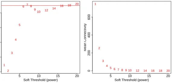
Constructing a weighted gene network entails the choice of the soft thresholding power β to which co-expression similarity is raised to calculate adjacency [1]. The authors of [1] have proposed to choose the soft thresholding power based on the criterion of approximate scale-free topology. We refer the reader to that work for more details; here we illustrate the use of the functionpickSoftThresholdthat performs the analysis of network topology and aids the user in choosing a proper soft-thresholding power. The user chooses a set of candidate powers (the function provides suitable default values), and the function returns a set of network indices that should be inspected, for example as follows:

# Choose a set of soft-thresholding powers

powers = c(c(1:10), seq(from = 12, to=20, by=2))

# Call the network topology analysis function

sft = pickSoftThreshold(datExpr, powerVector = powers, verbose = 5)

# Plot the results:

sizeGrWindow(9, 5) par(mfrow = c(1,2)); cex1 = 0.9;

# Scale-free topology fit index as a function of the soft-thresholding power

plot(sft$fitIndices[,1], -sign(sft$fitIndices[,3])*sft$fitIndices[,2],

xlab="Soft Threshold (power)",ylab="Scale Free Topology Model Fit,signed R^2",type="n", main = paste("Scale independence"));

text(sft$fitIndices[,1], -sign(sft$fitIndices[,3])*sft$fitIndices[,2], labels=powers,cex=cex1,col="red");

# this line corresponds to using an R^2 cut-off of h

abline(h=0.90,col="red")

# Mean connectivity as a function of the soft-thresholding power

plot(sft$fitIndices[,1], sft$fitIndices[,5],

xlab="Soft Threshold (power)",ylab="Mean Connectivity", type="n", main = paste("Mean connectivity"))

text(sft$fitIndices[,1], sft$fitIndices[,5], labels=powers, cex=cex1,col="red")

The result is shown in Fig. 1. We choose the power 6, which is the lowest power for which the scale-free topology fit index curve flattens out upon reaching a high value (in this case, roughly 0.90).

(3)

5 10 15 20 0.0 0.2 0.4 0.6 0.8 Scale independence

Soft Threshold (power)

Scale Free Topology Model Fit,signed R^2 1 2 3 4 5 6 7 8 9 10 12 14 16 18 20 5 10 15 20 0 200 400 600 Mean connectivity

Soft Threshold (power)

Mean Connectivity 1 2 3 4 5 6 7 8 9 10 12 14 16 18 20

Figure 1: Analysis of network topology for various soft-thresholding powers. The left panel shows the scale-free fit index (y-axis) as a function of the soft-thresholding power (x-axis). The right panel displays the mean connectivity (degree,y-axis) as a function of the soft-thresholding power (x-axis).

2.a.2 One-step network construction and module detection

Constructing the gene network and identifying modules is now a simple function call:

net = blockwiseModules(datExpr, power = 6,

TOMType = "unsigned", minModuleSize = 30, reassignThreshold = 0, mergeCutHeight = 0.25, numericLabels = TRUE, pamRespectsDendro = FALSE, saveTOMs = TRUE,

saveTOMFileBase = "femaleMouseTOM", verbose = 3)

We have chosen the soft thresholding power 6, a relatively large minimum module size of 30, and a medium sensitivity (deepSplit=2) to cluster splitting. The parametermergeCutHeightis the threshold for merging of modules. We have also instructed the function to return numeric, rather than color, labels for modules, and to save the Topological Overlap Matrix. The output of the function may seem somewhat cryptic, but it is easy to use. For example,

net$colorscontains the module assignment, andnet$MEscontains the module eigengenes of the modules.

A word of caution for the readers who would like to adapt this code for their own data. The function

blockwiseModules has many parameters, and in this example most of them are left at their default value. We

have attempted to provide reasonable default values, but they may not be appropriate for the particular data set the reader wishes to analyze. We encourage the user to read the help file provided within the package in the R envi-ronment and experiment with tweaking the network construction and module detection parameters. The potential reward is, of course, better (biologically more relevant) results of the analysis.

A second word of caution concerning block size. In particular, the parametermaxBlockSizetells the function how large the largest block can be that the reader’s computer can handle. The default value is 5000 which is appropriate for most modern desktops. Note that if this code were to be used to analyze a data set with more than 5000 probes, the function blockwiseModuleswill split the data set into several blocks. This will break some of the

plotting code below,that is executing the code will lead to errors. Readers wishing to analyze larger data sets need

(4)

• If the reader has access to a large workstation with more than 4 GB of memory, the parametermaxBlockSize

can be increased. A 16GB workstation should handle up to 20000 probes; a 32GB workstation should handle perhaps 30000. A 4GB standard desktop or a laptop may handle up to 8000-10000 probes, depending on operating system and ihow much memory is in use by other running programs.

• If a computer with large-enough memory is not available, the reader should follow Section 2.c,Dealing with

large datasets, and adapt the code presented there for their needs. In general it is preferable to analyze a data

set in one block if possible, although in Section 2.c we present a comparison of block-wise and single-block analysis that indicates that the results are very similar.

We now return to the network analysis. To see how many modules were identified and what the module sizes are, one can usetable(net$colors). Its output is

> table(net$colors)

0 1 2 3 4 5 6 7 8 9 10 11 12 13 14 15 16 17 18

99 609 460 409 316 312 221 211 157 123 106 100 94 91 77 76 58 47 34

and indicates that there are 18 modules, labeled 1 through 18 in order of descending size, with sizes ranging from 609 to 34 genes. The label 0 is reserved for genes outside of all modules.

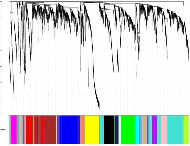
The hierarchical clustering dendrogram (tree) used for the module identification is returned innet$dendrograms[[1]]; #$. The dendrogram can be displayed together with the color assignment using the following code:

# open a graphics window

sizeGrWindow(12, 9)

# Convert labels to colors for plotting

mergedColors = labels2colors(net$colors)

# Plot the dendrogram and the module colors underneath

plotDendroAndColors(net$dendrograms[[1]], mergedColors[net$blockGenes[[1]]],

"Module colors",

dendroLabels = FALSE, hang = 0.03, addGuide = TRUE, guideHang = 0.05)

The resulting plot is shown in Fig. 2. We note that if the user would like to change some of the tree cut, module membership, and module merging criteria, the package provides the function recutBlockwiseTrees that can apply modified criteria without having to recompute the network and the clustering dendrogram. This may save a sub-stantial amount of time.

We now save the module assignment and module eigengene information necessary for subsequent analysis.

moduleLabels = net$colors

moduleColors = labels2colors(net$colors) MEs = net$MEs;

geneTree = net$dendrograms[[1]];

save(MEs, moduleLabels, moduleColors, geneTree,

file = "FemaleLiver-02-networkConstruction-auto.RData")

References

[1] B. Zhang and S. Horvath. A general framework for weighted gene co-expression network analysis. Statistical

(5)

0.3 0.4 0.5 0.6 0.7 0.8 0.9 1.0 Cluster Dendrogram hclust (*, "average") as.dist(dissTom) Height Module colors

Figure 2: Clustering dendrogram of genes, with dissimilarity based on topological overlap, together with assigned module colors.

Tutorial for the WGCNA package for R: I. Network analysis of liver expression data in female mice